

Abstract
Identifying B-cell epitopes play an important role in vaccine design, immunodiagnostic tests, and antibody production. Therefore, computational tools for reliably predicting B-cell epitopes are highly desirable. We explore two machine learning approaches for predicting flexible length linear B-cell epitopes. The first approach utilizes four sequence kernels for determining a similarity score between any arbitrary pair of variable length sequences. The second approach utilizes four different methods of mapping a variable length sequence into a fixed length feature vector. Based on our empirical comparisons, we propose FBCPred, a novel method for predicting flexible length linear B-cell epitopes using the subsequence kernel. Our results demonstrate that FBCPred significantly outperforms all other classifiers evaluated in this study. An implementation of FBCPred and the datasets used in this study are publicly available through our linear B-cell epitope prediction server, BCPREDS, at: http://ailab.cs.iastate.edu/bcpreds/.
1. INTRODUCTION
B-cell epitopes are antigenic determinants that are recognized and bound by receptors (membrane-bound antibodies) on the surface of B lymphocytes 1. The identification and characterization of B-cell epitopes play an important role in vaccine design, immunodiagnostic tests, and antibody production. As identifying B-cell epitopes experimentally is time-consuming and expensive, computational methods for reliably and efficiently predicting B-cell epitopes are highly desirable 2.
There are two types of B-cell epitopes: (i) linear (continuous) epitopes which are short peptides corresponding to a contiguous amino acid sequence fragment of a protein 3, 4; (ii) conformational (discontinuous) epitopes which are composed of amino acids that are not contiguous in primary sequence but are brought into close proximity within the folded protein structure. Although it is believed that a large majority of B-cell epitopes are discontinuous 5, experimental epitope identification has focused primarily on linear B-cell epitopes 6. Even in the case of linear B-cell epitopes, however, antibody-antigen interactions are often conformation-dependent. The conformation-dependent aspect of antibody binding complicates the problem of B-cell epitope prediction, making it less tractable than T-cell epitope prediction. Hence, the development of reliable computational methods for predicting linear B-cell epitopes is an important challenge in bioinformatics and computational biology 2.
Previous studies have reported correlations between certain physicochemical properties of amino acids and the locations of linear B-cell epitopes within protein sequences 7–11. Based on that observation, several amino acid propensity scale based methods have been proposed. For example, methods in 8–11 utilized hydrophilicity, flexibility, turns, and solvent accessibility propensity scales, respectively. PREDITOP 12, PEOPLE 13, BEPITOPE 14, and BcePred 15 utilized groups of physicochemical properties instead of a single property to improve the accuracy of the predicted linear B-cell epitopes. Unfortunately, Blythe and Flower 16 showed that propensity based methods can not be used reliably for predicting B-cell epitopes. Using a dataset of 50 proteins and an exhaustive assessment of 484 amino acid propensity scales, Blythe and Flower 16 showed that the best combinations of amino acid propensities performed only marginally better than random. They concluded that the reported performance of such methods in the literature is likely to have been overly optimistic, in part due to the small size of the data sets on which the methods had been evaluated.
Recently, the increasing availability of experimentally identified linear B-cell epitopes in addition to Blythe and Flower results 16 motivated several researchers to explore the application of machine learning approaches for developing linear B-cell epitope prediction methods. BepiPred 17 combines two amino acid propensity scales and a Hidden Markov Model (HMM) trained on linear epitopes to yield a slight improvement in prediction accuracy relative to techniques that rely on analysis of amino acid physicochemical properties. ABCPred 18 uses artificial neural networks for predicting linear B-cell epitopes. Both feed-forward and recurrent neural networks were evaluated on a non-redundant data set of 700 B-cell epitopes and 700 non-epitope peptides, using 5-fold cross validation tests. Input sequence windows ranging from 10 to 20 amino acids, were tested and the best performance, 66% accuracy, was obtained using a recurrent neural network trained on peptides 16 amino acids in length. In the method of Söllner and Mayer 19, each epitope is represented using a set of 1487 features extracted from a variety of propensity scales, neighborhood matrices, and respective probability and likelihood values. Of two machine learning methods tested, decision trees and a nearest-neighbor method combined with feature selection, the latter was reported to attain an accuracy of 72% on a data set of 1211 B-cell epitopes and 1211 non-epitopes, using a 5-fold cross validation test 19. Chen et al. 20 observed that certain amino acid pairs (AAPs) tend to occur more frequently in B-cell epitopes than in non-epitope peptides. Using an AAP propensity scale based on this observation, in combination with a support vector machine (SVM) classifier, they reported prediction accuracy of 71% on a data set of 872 B-cell epitopes and 872 non-B-cell epitopes, estimated using 5-fold cross validation. In addition, 20 demonstrated an improvement in the prediction accuracy, 72.5%, when the APP propensity scale is combined with turns accessibility, antigenicity, hydrophilicity, and flexibility propensity scales.
Existing linear B-cell epitope prediction tools fall into two broad categories. Tools in the first category, residue-based predictors, take as input a protein sequence and assign binary labels to each individual residue in the input sequence. Each group of neighboring residues with predicted positive labels define a variable length predicted linear B-cell epitope. Residue-based prediction methods scan the input sequence using a sliding window and assign a score to the amino acid at the center of the window based on the mean score of a certain propensity scale (e.g., flexibility or hydrophilicity). The target residue is predicted positive if its score is greater than a predetermined threshold. Unfortunately, it has been shown that the performance of these methods is marginally better than random 16. PepiPred 17 used the information extracted using the sliding window to train a HMM and combined it with two propensity scale based methods. BcePred 15 combined several propensity scales and showed that the performance of the combined scales is better than the performance of any single scale.
The second category of linear B-cell prediction tools consist of the epitope-based predictors. An example of such predictors is the ABCPred server 18. For this server, the input is a protein sequence and an epitope length (should be in {20, 18, .., 10}). The server then applies a sliding window of the user specified length and passes the extracted peptides to a neural network classifier trained using epitope dataset in which all the epitope sequences have been set to the specified epitope length via trimming and extending longer and shorter epitopes, respectively. A limitation of this approach is that the user is forced to select one of the available six possible epitope lengths and can not specify a different epitope length.
Because linear B-cell epitopes can vary in length over a broad range (see Figure 1), it is natural to train classifiers using the experimentally reported epitope sequences without trimming or extending them. Such an approach will allow us to provide a linear B-cell epitope prediction tool that allows the user to experiment with virtually any arbitrary epitope length. In this work, we explore two machine learning approaches for predicting flexible length linear B-cell epitopes. The first approach utilizes several sequence kernels for determining a similarity score between any arbitrary pair of variable length sequences. The second approach utilizes many different methods of mapping a variable length sequence into a fixed length feature vector. Based on our empirical comparisons, we propose FBCPred, a novel method for predicting flexible length linear B-cell epitopes using the subsequence kernel. Our results demonstrate that FBCPred significantly outperforms all other classifiers evaluated in this study. An implementation of FBCPred and the datasets used in this study are publicly available through our linear B-cell epitope prediction server, BCPREDS, at: http://ailab.cs.iastate.edu/bcpreds/.
Fig. 1.
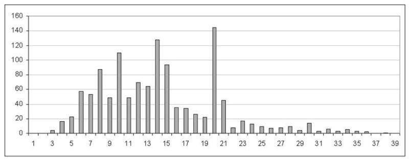
Length distribution of unique linear B-cell epitopes in Bcipep database.
2. MATERIALS AND METHODS
2.1. Data
We retrieved 1223 unique linear B-cell epitopes of lengths more than 3 amino acids from Bcipep database 21. To avoid over-optimistic performance of classifiers evaluated on the set of unique epitopes, we applied a homology reduction procedure proposed by Raghava 22 for reducing sequence similarity among flexible length major histocompatibility complex class II (MHC-II) peptides. Briefly, given two peptides p1 and p2 of lengths l1 and l2 such that l1 l2, we compare p1 with each l1-length subpeptide in p2. If the percent identity (PID) between p1 and any subpeptide in p2 is greater than 80%, then the two peptides are deemed to be similar. For example, to compute the PID between (ACDEFGHIKLMNPQRST) and (DEFGGIKLMN), we compare (DEFGGIKLMN) with (ACDEFGHIKL), (CDEFGHIKLM), …, (IKLMNPQRST). The PID between (DEFGGIKLMN) and (DEFGHIKLMN) is 90% since nine out of 10 residues are identical.
Applying the above homology reduction procedure to the set of 1223 unique variable length linear B-cell epitopes yields a homology-reduced set of 934 epitopes. Two datasets of flexible length linear B-cell epitopes have been constructed. An original dataset constructed from the set of 1223 unique epitopes as the positive examples and 1223 non-epitopes randomly extracted from SwissProt 23 and a homology-reduced dataset constructed from homology-reduced set of 934 epitopes as positive examples and an equal number of negative examples extracted randomly form SwissProt sequences. In both datasets two selection criteria have been applied to the randomly extracted non-epitopes: (i) the length distribution in the negative data is identical to the length distribution in the positive data; (ii) none of the non-epitopes appears in the set of epitopes.
2.2. Support vector machines and kernel methods
Support vector machines (SVMs) 24 are a class of supervised machine learning methods used for classification and regression. Given a set of labeled training data (xi, yi), where xi ∈ Rd and yi ∈ {+1, −1}, training an SVM classifier involves finding a hyperplane that maximizes the geometric margin between positive and negative training data samples. The hyperplane is described as f (x) = 〈w, x〉 + b, where w is a normal vector and b is a bias term. A test instance, x, is assigned a positive label if f (x) > 0, and a negative label otherwise. When the training data are not linearly separable, a kernel function is used to map nonlinearly separable data from the input space into a feature space. Given any two data samples xi and xj in an input space X ∈ Rd, the kernel function K returns K(xi, xj) = 〈(xi), (xj)〉 where is a nonlinear map from the input space X to the corresponding feature space. The kernel function K has the property that K(xi, xj) can be computed without explicitly mapping xi and xj into the feature space, but instead, using their dot product 〈xi, xj〉 in the input space. Therefore, the kernel trick allows us to train a linear classifier, e.g., SVM, in a high-dimensional feature space where the data are assumed to be linearly separable without explicitly mapping each training example from the input space into the feature space. This approach relies implicitly on the selection of a feature space in which the training data are likely to be linearly separable (or nearly so) and explicitly on the selection of the kernel function to achieve such separability. Unfortunately, there is no single kernel that is guaranteed to perform well on every data set. Consequently, the SVM approach requires some care in selecting a suitable kernel and tuning the kernel parameters (if any).
2.3. Sequence kernel based methods
String kernels 25–29 are a class of kernel methods that have been successfully used in many sequence classification tasks 25, 26, 28, 30–32. In these applications, a protein sequence is viewed as a string defined on a finite alphabet of 20 amino acids. In this work, we explore four string kernels: spectrum 25, mismatch 26, local alignment 28, and subsequence 27, in predicting linear B-cell epitopes. A brief description of the four kernels follows.
2.3.1. Spectrum kernel
Let A denote a finite alphabet, e.g., the standard 20 amino acids. x and y denote two strings defined on the alphabet A. For k ≥ 1, the k-spectrum is defined as 25:
| (1) |
where φα is the number of occurrences of the k-length substring α in the sequence x. The k-spectrum kernel of the two sequences x and y is obtained by taking the dot product of the corresponding k spectra:
| (2) |
The k-spectrum kernel captures a simple notion of string similarity: two strings are deemed similar (i.e., have a high k-spectrum kernel value) if they share many of the same k-length substrings.
2.3.2. Mismatch kernel
The mismatch kernel 26 is a variant of the spectrum kernel in which inexact matching is allowed. Specifically, the (k, m)-mismatch kernel allows up to m k mismatches to occur when comparing two k-length substrings. Let α be a k-length substring, the (k, m)-mismatch feature map is defined on α as:
| (3) |
where φβ (α) = 1 if β ∈ N(k,m)(α), where β is the set of k-mer substrings that differs from α by at most m mismatches. Then, the feature map of an input sequence x is the sum of the feature vectors for k-mer substrings in x:
| (4) |
The (k, m)-mismatch kernel is defined as the dot product of the corresponding feature maps in the feature space:
| (5) |
It should be noted that the (k, 0)-mismatch kernel results in a feature space that is identical to that of the k-spectrum kernel. An efficient data structure for computing the spectrum and mismatch kernels in O(|x|+ |y|) and O(km+1|A|m(|x|+ |y|)), respectively, is provided in 26.
2.3.3. Local alignment kernel
Local alignment (LA) kernel 28 is a string kernel adapted for biological sequences. The LA kernel measures the similarity between two sequences by summing up scores obtained from gapped local alignments of the sequences. This kernel has several parameters: the gap opening and extension penalty parameters, d and e, the amino acid mutation matrix s, and the factor β, which controls the influence of suboptimal alignments on the kernel value. Detailed formulation of the LA kernel and a dynamic programming implementation of the kernel with running time complexity in O(|x||y|) are provided in 28.
2.3.4. Subsequence kernel
The subsequence kernel (SSK) 27 generalizes the k-spectrum kernel by considering a feature space generated by the set of all (contiguous and non-contiguous) k-mer subsequences. For example, if we consider the two strings “act” and “acctct”, the value returned by the spectrum kernel with k = 3 is 0. On the other hand, the (3, 1)-mismatch kernel will return 3 because the 3-mer substrings “acc”, “cct”, and “tct” have at most one mismatch when compared with “act”. The subsequence kernel considers the set (“ac – t”, “a – ct”, “ac – – – t”, “a – c – –t”, “a – – – ct”) of non-contiguous substrings and returns a similarity score that is weighted by the length of each non-contiguous substring. Specifically, it uses a decay factor, λ 1, to penalize non-contiguous substring matches. Therefore, the subsequence kernel with k = 3 will return 2λ4 + 3λ6 when applied to “act” and “acctct” strings. More precisely, the feature map (k,λ) of a string x is given by:
| (6) |
where u = x[i] denotes a substring in x where 1 i1 < … < i|u| |x| such that uj = sij, for j = 1, …, |u| and l(i) = i|u| − i1 + 1 is the length of the subsequence in x. The subsequence kernel for two strings x and y is determined as the dot product of the corresponding feature maps:
| (7) |
This kernel can be computed using a recursive algorithm based on dynamic programming in O(k|x||y|) time and space. The running time and memory requirements can be further reduced using techniques described in 33.
2.4. Sequence-to-features based methods
This approach has been previously used for protein function and structure classification tasks 34–37 and the classification of flexible length MHC-II peptides. The main idea is to map each variable length amino acid sequence into a feature vector of fixed length. Once the variable length sequences are mapped to fixed length feature vectors, we can apply any of the standard machine learning algorithms to this problem. Here, we considered SVM classifiers trained on the mapped data using the widely used RBF kernel.
We explored four different methods for mapping a variable length amino acid sequence into a fixed length feature vector: (i) amino acid composition; (ii) dipeptide composition; (iii) amino acid pairs propensity scale; (iv) composition-transition-distribution. A brief summary of each method is given below.
2.4.1. Amino acid and dipeptide composition
Amino acid composition (AAC) represents a variable length amino acid sequence using a feature vector of 20 dimensions. Let x be a sequence of |x| amino acids. Let A denote the set of the standard 20 amino acids. The amino acid composition feature mapping is defined as:
| (8) |
where .
A limitation of the amino acid composition feature representation of amino acid sequences is that we lose the sequence order information. Dipeptide composition (DC) encapsulates information about the fraction of amino acids as well as their local order. In dipeptide composition each variable length amino acid sequence is represented by a feature vector of 400 dimensions defined as:
| (9) |
where .
2.4.2. Amino acid pairs propensity scale
Amino acid pairs (AAPs) are obtained by decomposing a protein/peptide sequence into its 2-mer subsequences. 20 observed that some specific AAPs tend to occur more frequently in B-cell epitopes than in non-epitope peptides. Based on this observation, they developed an AAP propensity scale defined by:
| (10) |
where and are the occurrence frequencies of AAP α in the epitope and non-epitope peptide sequences, respectively. These frequencies have been derived from Bcipep 21 and Swissprot 23 databases, respectively. To avoid the dominance of an individual AAP propensity value, the scale in Eq. (10) has been normalized to a [−1, +1] interval through the following conversion:
| (11) |
where max and min are the maximum and minimum values of the propensity scale before the normalization.
The AAP feature mapping, AAP, maps each amino acid sequence, x, into a 400-dimentional feature space defined as:
| (12) |
where φα(x) is the number of occurrences of the 2-mer α in the peptide x.
2.4.3. Composition-Transition-Distribution
The basic idea behind the Composition-Transition-Distribution (CTD) method 38, 39 is to map each variable length peptide into a fixed length feature vector such that standard machine learning algorithms are applicable. From each peptide sequence, 21 features are extracted as follows:
First, each peptide sequence p is mapped into a string sp defined over an alphabet of three symbols, {1, 2, 3}. The mapping is performed by grouping amino acids into three groups using a physicochemical property of amino acids (see Table 3). For example the peptide (AIRHIPRRIR) is mapped into (2312321131) using the hydrophobicity division of amino acids into three groups (see Table 3).
-
Second, for each peptide string sp, three descriptors are derived as follows:
Composition (C): three features representing the percent frequency of the symbols, {1, 2, 3}, in the mapped peptide sequence.
Transition (T): three features representing the percent frequency of i followed by j or j followed by i, for i, j ∈ {1, 2, 3}.
Distribution (D): five features per symbol representing the fractions of the entire sequence where the first, 25, 50, 75, and 100% of the candidate symbol are contained in sp. This yields an additional 15 features for each peptide.
Table 3.
Performance of different SVM based classifiers on homology-reduced dataset of flexible length linear B–cell epitopes. Results are the average of 10 runs of 5-fold cross validation.
| Method | ACC | Sn | Sp | CC | AUC | |
|---|---|---|---|---|---|---|
|
|
58.22 | 56.70 | 59.74 | 0.165 | 0.621 | |
|
|
60.26 | 61.04 | 59.49 | 0.205 | 0.642 | |
|
|
60.86 | 62.45 | 59.27 | 0.217 | 0.635 | |
|
|
46.42 | 46.34 | 46.50 | −0.072 | 0.451 | |
|
|
54.35 | 54.75 | 53.95 | 0.087 | 0.561 | |
| LA | 61.38 | 60.41 | 62.35 | 0.228 | 0.658 | |
|
|
60.09 | 60.52 | 59.66 | 0.202 | 0.647 | |
|
|
63.85 | 65.05 | 62.65 | 0.277 | 0.701 | |
|
|
65.49 | 68.36 | 62.61 | 0.310 | 0.738 | |
|
| ||||||
| AAC | 63.31 | 70.90 | 55.73 | 0.269 | 0.683 | |
| DC | 63.78 | 63.05 | 64.51 | 0.276 | 0.667 | |
| AAP | 61.42 | 62.85 | 60.00 | 0.229 | 0.658 | |
| CTD | 60.32 | 59.66 | 60.98 | 0.206 | 0.639 | |
Table 1 shows division of the 20 amino acids, proposed by Chinnasamy et al. 40, into three groups based on hydrophobicity, polarizability, polarity, and Van der Waal’s volume properties. Using these four properties, we derived 84 CTD features from each peptide sequence. In our experiments, we trained SVM classifiers using RBF kernel and peptide sequences represented using their amino acid sequence composition (20 features) and CTD descriptors (84 features).
Table 1.
Categorization of amino acids into three groups for a number of physicochemical properties.
| Proporty | Group 1 | Group 2 | Group 3 |
|---|---|---|---|
| Hydrophobicity | RKEDQN | GASTPHY | CVLIMFW |
| Polarizability | GASCTPD | NVEQIL | MHKFRYW |
| Polarity | LIFWCMVY | PATGS | HQRKNED |
| Van der Waala volume | GASDT | CPNVEQIL | KMHFRYW |
2.5. Performance evaluation
We report the performance of each classifier using the average of 10 runs of 5-fold cross validation tests. Each classifier performance is assessed by both threshold-dependent and threshold-independent metrics. For threshold-dependent metrics, we used accuracy (ACC), sensitivity (Sn), specificity (Sp), and correlation coefficient (CC). The CC measure has a value in the range from −1 to +1 and the closer the value to +1, the better the predictor. The Sn and Sp summarize the accuracies of the positive and negative predictions respectively. ACC, Sn, Sp, and CC are defined in Eq. (13–15) where TP, FP, TN, FN are the numbers of true positives, false positives, true negatives, and false negatives respectively.
For threshold-independent metrics, we report the Receiver Operating Characteristic (ROC) curve. The ROC curve is obtained by plotting the true positive rate as a function of the false positive rate or, equivalently, sensitivity versus (1-specificity) as the discrimination threshold of the binary classifier is varied. Each point on the ROC curve describes the classifier at a certain threshold value and hence a particular choice of tradeoff between true positive rate and false negative rate. We also report the area under ROC curve (AUC) as a useful summary statistic for comparing two ROC curves. AUC is defined as the probability that a randomly chosen positive example will be ranked higher than a randomly chosen negative example. An ideal classifier will have an AUC = 1, while a classifier performs no better than random will have an AUC = 0.5, any classifier performing better than random will have an AUC value that lies between these two extremes.
2.6. Implementation and SVM parameter optimization
We used Weka machine learning workbench 41 for implementing the spectrum, mismatch, and LA kernels (RBF and SSK kernels are already implemented in Weka). We evaluated the k-spectrum kernel, , for k = 1, 2, and 3. The (k, m)-mismatch kernel was evaluated at (k,m) equals (3, 1)and(4, 1). The subsequence kernel, , was evaluated at k = 2, 3, and 4 and the default value for λ, 0.5. The LA kernel was evaluated using the BLOSUM62 substitution matrix, gap opening and extension parameters equal to 10 and 1, respectively, and β = 0.5. For the SVM classifier, we used the Weka implementation of the SMO 42 algorithm. For the string kernels, the default value of the C parameter, C = 1, was used for the SMO classifier. For methods that uses the RBF kernel, we found that tuning the SMO cost parameter C and the RBF kernel parameter γ is necessary to obtain satisfactory performance. We tuned these parameters using a 2-dimensional grid search over the range C = 2−5, 2−3, …, 23, γ = 2−15, 2−13, …, 23.
3. RESULTS AND DISCUSSION
Table 2 compares the performance of different SVM based classifiers on the original dataset of unique flexible length linear B-cell epitopes. The SVM classifier trained using SSK with k = 4 and λ = 0.5, , significantly (using statistical paired t-test 43 with p-value = 0.05) outperforms all other classifiers in terms of the AUC. The two classifiers based on the mismatch kernel have the worst AUC. The classifier trained using is competitive to those trained using the LA kernel and . The last four classifiers belong to the sequence-to-feature approach. Each of these classifiers has been trained using an SVM classifier and the RBF kernel but on different data representation. The results suggest that representation of
Table 2.
Performance of different SVM based classifiers on original dataset of unique flexible length linear B-cell epitopes. Results are the average of 10 runs of 5-fold cross validation.
| Method | ACC | Sn | Sp | CC | AUC | |
|---|---|---|---|---|---|---|
|
|
62.86 | 61.76 | 63.95 | 0.257 | 0.680 | |
|
|
63.29 | 63.84 | 62.74 | 0.266 | 0.683 | |
|
|
65.36 | 79.28 | 51.44 | 0.320 | 0.720 | |
|
|
47.88 | 48.42 | 47.33 | −0.042 | 0.480 | |
|
|
58.93 | 57.79 | 60.07 | 0.179 | 0.618 | |
| LA | 65.41 | 63.36 | 67.46 | 0.308 | 0.716 | |
|
|
65.58 | 65.08 | 66.09 | 0.312 | 0.710 | |
|
|
70.56 | 71.05 | 70.07 | 0.411 | 0.778 | |
|
|
73.37 | 74.08 | 72.67 | 0.468 | 0.812 | |
|
| ||||||
| AAC | 65.61 | 68.41 | 62.81 | 0.313 | 0.722 | |
| DC | 70.55 | 68.28 | 72.83 | 0.411 | 0.750 | |
| AAP | 65.65 | 66.20 | 65.11 | 0.313 | 0.717 | |
| CTD | 63.21 | 63.15 | 63.28 | 0.264 | 0.686 | |
| (13) |
| (14) |
| (15) |
the peptides using their dipeptide composition performs better than other feature representations on the original dataset. Figure 2 shows the ROC curves for different methods on original dataset of unique flexible length linear B-cell epitopes. The ROC curve of based classifier almost dominates all other ROC curves (i.e., for any choice of specificity value, the based classifier almost has the best sensitivity).
Fig. 2.
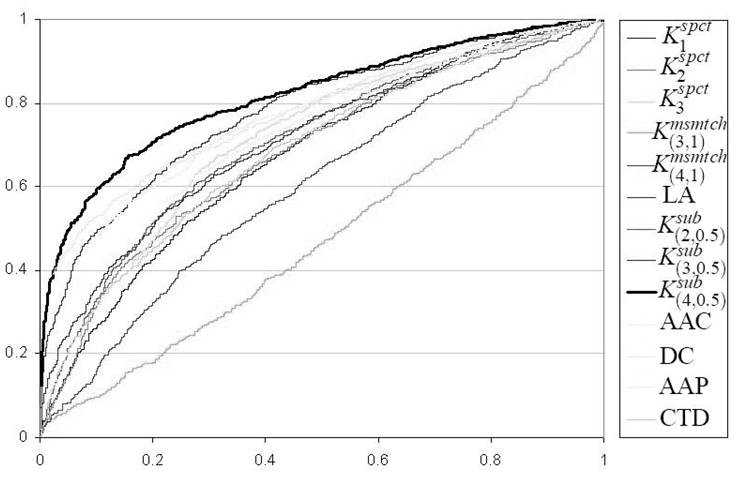
ROC curves for different methods on original dataset of unique flexible length linear B-cell epitopes. The ROC curve of based classifier almost dominates all other ROC curves.
Table 3 reports the performance of the different SVM based classifiers on the homology-reduced dataset of flexible length linear B-cell epitopes. We note that the performance of each classifier is considerably worse than its performance on the original dataset of unique epitopes. This discrepancy can be explained by the existence of epitopes with significant pairwise sequence similarity in the original dataset. Interestingly, the SVM classifier based on the kernel still significantly outperforms all other classifiers at 0.05 level of significance. Figure 3 shows the ROC curves for different methods on homology-reduced dataset of flexible length linear B-cell epitopes. Again, the ROC curve of based classifier almost dominates all other ROC curves.
Fig. 3.
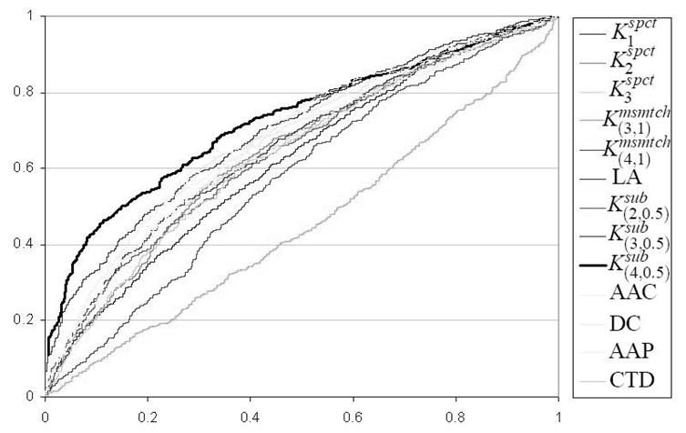
ROC curves for different methods on homology-reduced dataset of flexible length linear B-cell epitopes. The ROC curve of based classifier almost dominates all other ROC curves.
Comparing results on Table 2 and Table 3 reveals two important issues that to the best of our knowledge have not been addressed before in the literature on B-cell epitope prediction. First, our results demonstrate that performance estimates reported on the basis of the original dataset of unique linear B-cell epitopes is overly optimistic compared to the performance estimates obtained using the homology-reduced dataset. Hence, we suspect that the actual performance of linear B-cell epitope prediction methods on homology-reduced datasets is somewhat lower than the reported performance on the original dataset of unique peptides. Second, our results suggest that conclusions regarding how different prediction methods compare to each other drawn on the basis of datasets of unique epitopes may be misleading. For example, from the reported results in Table 2, one may conclude that outperforms and while results on the homology-reduced dataset (see Table 3) demonstrate that the three classifiers are competitive with each other. Another example of misleading conclusions drawn from results in Table 2 is that dipeptide composition features is a better representation than amino acid composition representation of the data. This conclusion is contradicted by results in Table 3 which show that the classifier constructed using the amino acid composition representation of the data slightly outperforms the classifier constructed using the dipeptide composition of the same data.
The results in Table 2 and Table 3 show that the classifier that used the amino acid composition features outperforms the classifier that used CTD features. This is interesting because the set of amino acid composition features is a subset of the CTD features. Recall that CTD is composed of 20 amino acid composition features plus 84 physicochemical features, we conclude that the added physicochemical features did not yield additional information that was relevant for the classification task. In addition, we observed that the classifier that used the dipeptide composition outperforms the classifier that used the AAP features. This is interesting because AAP features as defined in Eq. (12) can be viewed as dipeptide composition features weighted by the amino acid propensity of each dipeptide.
3.1. Web server
An implementation of FBCPred is available as a part of our B-cell epitope prediction server (BCPREDS) 44 which is freely accessible at http://ailab.cs.iastate.edu/bcpreds/. Because it is often valuable to compare predictions of multiple methods, and consensus predictions are more reliable than individual predictions, the BCPREDS server aims at providing predictions using several B-cell epitope prediction methods. The current implementation of BCPREDS allows the user to select among three prediction methods: (i) Our implementation of AAP method 20; (ii) BCPred 44, a method for predicting linear B-cell epitope using the subsequence kernel; (iii) FBCPred, the method introduced in this study for predicting flexible length B-cell epitopes. The major difference between FBCPred and the other two methods is that FBCPred can predict linear B-cell epitopes of virtually any arbitrary length while for the other two methods the length has to be one of possible six values, {12, 14, …, 22}.
Another goal of BCPREDS server is to serve as a repository of benchmark B-cell epitope datasets. The datasets used for training and evaluating BCPred and the two datasets used in this study can be freely downloaded from the web server.
4. SUMMARY AND DISCUSSION
We explored two machine learning approaches for predicting flexible length linear B-cell epitopes. The first approach utilizes sequence kernels for determining a similarity score between any arbitrary pair of variable length sequences. The second approach utilizes several methods of mapping a variable length sequence into a fixed length feature vector. Our results demonstrated a superior performance of the subsequence kernel based SVM classifier compared to other SVM classifiers examined in our study. Therefore, we proposed FBCPred, a novel method for predicting flexible length linear B-cell epitopes using the subsequence kernel. An implementation of FBCPred and the datasets used in this study are publicly available through our linear B-cell prediction server, BCPREDS, at: http://ailab.cs.iastate.edu/bcpreds/.
Previous methods for predicting linear B-cell epitopes (e.g., 15, 17, 19, 18, 20) have been evaluated on datasets of unique epitopes without applying any homology reduction procedure as a pre-processing step on the data. We showed that performance estimates reported on the basis of such datasets is considerably over-optimistic compared to performance estimates obtained using the homology-reduced datasets. Moreover, we showed that using such non homology-reduced datasets for comparing different prediction methods may lead to false conclusions regarding how these methods compare to each other.
4.1. Related work
Residue-based prediction methods 7–11, 15, 17 assign labels to each residue in the query sequence and therefore are capable of predicting linear B-cell epitopes of variable length. However, most of these methods have been shown to be of low to moderate performance 16.
AAP method 20 maps each peptide sequence into a set of fixed length numeric features and therefore it can be trained using datasets of flexible length sequences. However, the performance of this method had been reported using a dataset of 20-mer peptides.
Söllner and Mayer 19 introduced a method for mapping flexible length epitope sequences into feature vectors of 1478 attributes. This method has been evaluated on a dataset of flexible length linear B-cell epitopes. However, no homology reduction procedure was applied to remove highly similar sequences from the data. In addition, the implementation of this method is not publicly available.
Recently, two methods 45, 39 have been successfully applied to the problem of predicting flexible length MHC-II binding peptides. The first method 45 utilized the LA kernel 28 for developing efficient SVM based classifiers. The second method 39 mapped each flexible length peptide into the set of CTD features employed in our study in addition to some extra features extracted using two secondary structure and solvent accessibility prediction classifiers. In our study we could not use these extra features due to the unavailability of these two programs.
Acknowledgments
This work was supported in part by a doctoral fellowship from the Egyptian Government to Yasser EL-Manzalawy and a grant from the National Institutes of Health (GM066387) to Vasant Honavar and Drena Dobbs.
Contributor Information
Yasser EL-Manzalawy, Email: yasser@iastate.edu.
Drena Dobbs, Email: ddobbs@iastate.edu.
Vasant Honavar, Email: honavar@iastate.edu.
References
- 1.Pier GB, Lyczak JB, Wetzler LM. Immunology, infection, and immunity. 1. ASM Press; PL Washington: 2004. [Google Scholar]
- 2.Greenbaum JA, Andersen PH, Blythe M, Bui HH, Cachau RE, Crowe J, Davies M, Kolaskar AS, Lund O, Morrison S, et al. Towards a consensus on datasets and evaluation metrics for developing B-cell epitope prediction tools. J Mol Recognit. 2007;20:75–82. doi: 10.1002/jmr.815. [DOI] [PubMed] [Google Scholar]
- 3.Barlow DJ, Edwards MS, Thornton JM, et al. Continuous and discontinuous protein antigenic determinants. Nature. 1986;322:747–748. doi: 10.1038/322747a0. [DOI] [PubMed] [Google Scholar]
- 4.Langeveld JP, martinez Torrecuadrada J, boshuizen RS, Meloen RH, Ignacio CJ. Characterisation of a protective linear B cell epitope against feline parvoviruses. Vaccine. 2001;19:2352–2360. doi: 10.1016/s0264-410x(00)00526-0. [DOI] [PubMed] [Google Scholar]
- 5.Walter G. Production and use of antibodies against synthetic peptides. J Immunol Methods. 1986;88:149–61. doi: 10.1016/0022-1759(86)90001-3. [DOI] [PubMed] [Google Scholar]
- 6.Flower DR. Immunoinformatics: Predicting immunogenicity in silico. 1. Humana; Totowa NJ: 2007. [DOI] [PubMed] [Google Scholar]
- 7.Pellequer JL, Westhof E, Van Regenmortel MH. Predicting location of continuous epitopes in proteins from their primary structures. Meth Enzymol. 1991;203:176–201. doi: 10.1016/0076-6879(91)03010-e. [DOI] [PubMed] [Google Scholar]
- 8.Parker JMR, Hodges RS, Guo D. New hydrophilicity scale derived from high-performance liquid chromatography peptide retention data: correlation of predicted surface residues with antigenicity and x-ray-derived accessible sites. Biochemistry. 1986;25:5425–5432. doi: 10.1021/bi00367a013. [DOI] [PubMed] [Google Scholar]
- 9.Karplus PA, Schulz GE. Prediction of chain flexibility in proteins: a tool for the selection of peptide antigen. Naturwiss. 1985;72:21–213. [Google Scholar]
- 10.Emini EA, Hughes JV, Perlow DS, Boger J. Induction of hepatitis A virus-neutralizing antibody by a virus-specific synthetic peptide. J Virol. 1985;55:836–839. doi: 10.1128/jvi.55.3.836-839.1985. [DOI] [PMC free article] [PubMed] [Google Scholar]
- 11.Pellequer JL, Westhof E, Van Regenmortel MH. Correlation between the location of antigenic sites and the prediction of turns in proteins. Immunol Lett. 1993;36:83–99. doi: 10.1016/0165-2478(93)90072-a. [DOI] [PubMed] [Google Scholar]
- 12.Pellequer JL, Westhof E. PREDITOP: a program for antigenicity prediction. J Mol Graph. 1993;11:204–210. doi: 10.1016/0263-7855(93)80074-2. [DOI] [PubMed] [Google Scholar]
- 13.Alix AJ. Predictive estimation of protein linear epitopes by using the program PEOPLE. Vaccine. 1999;18:311–314. doi: 10.1016/s0264-410x(99)00329-1. [DOI] [PubMed] [Google Scholar]
- 14.Odorico M, Pellequer JL. BEPITOPE: predicting the location of continuous epitopes and patterns in proteins. J Mol Recognit. 2003;16:20–22. doi: 10.1002/jmr.602. [DOI] [PubMed] [Google Scholar]
- 15.Saha S, Raghava GP. BcePred: Prediction of continuous B-cell epitopes in antigenic sequences using physicochemical properties. Artificial Immune Systems, Third International Conference (ICARIS 2004) LNCS. 2004;3239:197–204. [Google Scholar]
- 16.Blythe MJ, Flower DR. Benchmarking B cell epitope prediction: Underperformance of existing methods. Protein Sci. 2005;14:246–248. doi: 10.1110/ps.041059505. [DOI] [PMC free article] [PubMed] [Google Scholar]
- 17.Larsen JE, Lund O, Nielsen M. Improved method for predicting linear B-cell epitopes. Immunome Res. 2006;2:2. doi: 10.1186/1745-7580-2-2. [DOI] [PMC free article] [PubMed] [Google Scholar]
- 18.Saha S, Raghava GP. Prediction of continuous B-cell epitopes in an antigen using recurrent neural network. Proteins. 2006;65:40–48. doi: 10.1002/prot.21078. [DOI] [PubMed] [Google Scholar]
- 19.Söllner J, Mayer B. Machine learning approaches for prediction of linear B-cell epitopes on proteins. J Mol Recognit. 2006;19:200–208. doi: 10.1002/jmr.771. [DOI] [PubMed] [Google Scholar]
- 20.Chen J, Liu H, Yang J, Chou KC. Prediction of linear B-cell epitopes using amino acid pair antigenicity scale. Amino Acids. 2007;33:423–428. doi: 10.1007/s00726-006-0485-9. [DOI] [PubMed] [Google Scholar]
- 21.Saha S, Bhasin M, Raghava GP. Bcipep: a database of B-cell epitopes. BMC Genomics. 2005;6:79. doi: 10.1186/1471-2164-6-79. [DOI] [PMC free article] [PubMed] [Google Scholar]
- 22.Raghava GPS. MHCBench: Evaluation of MHC Binding Peptide Prediction Algorithms. datasets available at http://www.imtech.res.in/raghava/mhcbench/
- 23.Bairoch A, Apweiler R. The SWISS-PROT protein sequence database and its supplement TrEMBL in 2000. Nucleic Acids Res. 2000;28:45–48. doi: 10.1093/nar/28.1.45. [DOI] [PMC free article] [PubMed] [Google Scholar]
- 24.Vapnik VN. The nature of statistical learning theory. 2. Springer-Verlag New York Inc; New York, USA: 2000. [Google Scholar]
- 25.Leslie C, Eskin E, Noble WS. The spectrum kernel: A string kernel for SVM protein classification. Proceedings of the Pacific Symposium on Biocomputing. 2002;7:566–575. [PubMed] [Google Scholar]
- 26.Leslie CS, Eskin E, Cohen A, Weston J, Noble WS. Mismatch string kernels for discriminative protein classification. Bioinformatics. 2004;20:467–476. doi: 10.1093/bioinformatics/btg431. [DOI] [PubMed] [Google Scholar]
- 27.Lodhi H, Saunders C, Shawe-Taylor J, Cristianini N, Watkins C. Text classification using string kernels. J Mach Learn Res. 2002;2:419–444. [Google Scholar]
- 28.Saigo H, Vert JP, Ueda N, Akutsu T. Protein homology detection using string alignment kernels. Bioinformatics. 2004;20:1682–1689. doi: 10.1093/bioinformatics/bth141. [DOI] [PubMed] [Google Scholar]
- 29.Haussler D. UC Santa Cruz Technical Report UCS-CRL-99-10. 1999. Convolution kernels on discrete structures. [Google Scholar]
- 30.Zaki NM, Deris S, Illias R. Application of string kernels in protein sequence classification. Appl Bioinformatics. 2005;4:45–52. doi: 10.2165/00822942-200504010-00005. [DOI] [PubMed] [Google Scholar]
- 31.Rangwala H, DeRonne K, Karypis G Minnesota Univ. Minneapolis Dept. of Computer Science. Protein structure prediction using string kernels. Defense Technical Information Center; 2006. [Google Scholar]
- 32.Wu F, Olson B, Dobbs D, Honavar V. Comparing kernels for predicting protein binding sites from amino acid sequence; International Joint Conference on Neural Networks (IJCNN06); 2006. pp. 1612–1616. [Google Scholar]
- 33.Seewald AK, Kleedorfer F. Technical report, Technical Report. Osterreichisches Forschungsinstitut fur Artificial Intelligence; Wien: 2005. Lambda pruning: An approximation of the string subsequence kernel. TR-2005-13. [Google Scholar]
- 34.Hua S, Sun Z. Support vector machine approach for protein subcellular localization prediction. Bioinformatics. 2001;17:721–728. doi: 10.1093/bioinformatics/17.8.721. [DOI] [PubMed] [Google Scholar]
- 35.Dobson PD, Doig AJ. Distinguishing Enzyme Structures from Non-enzymes Without Alignments. J Mol Biol. 2003;330:771–783. doi: 10.1016/s0022-2836(03)00628-4. [DOI] [PubMed] [Google Scholar]
- 36.Eisenhaber F, Frommel C, Argos P. Prediction of secondary structural content of proteins from their amino acid composition alone. II. The paradox with secondary structural class. Proteins. 1996;25:169–79. doi: 10.1002/(SICI)1097-0134(199606)25:2<169::AID-PROT3>3.0.CO;2-D. [DOI] [PubMed] [Google Scholar]
- 37.Luo R, Feng Z, Liu J. Prediction of protein structural class by amino acid and polypeptide composition. FEBS J. 2002;269:4219–4225. doi: 10.1046/j.1432-1033.2002.03115.x. [DOI] [PubMed] [Google Scholar]
- 38.Cai CZ, Han LY, Ji ZL, Chen X, Chen YZ. SVM-Prot: web-based support vector machine software for functional classification of a protein from its primary sequence. Nucleic Acids Res. 2003;31:3692–3697. doi: 10.1093/nar/gkg600. [DOI] [PMC free article] [PubMed] [Google Scholar]
- 39.Cui J, Han LY, Lin HH, Tan ZQ, Jiang L, Cao ZW, Chen YZ. MHC-BPS: MHC-binder prediction server for identifying peptides of flexible lengths from sequence-derived physicochemical properties. Immunogenetics. 2006;58:607–613. doi: 10.1007/s00251-006-0117-2. [DOI] [PubMed] [Google Scholar]
- 40.Chinnasamy A, Sung WK, Mittal A. Protein structure and fold prediction using tree-augmented naive Bayesian classifier. Pac Symp Biocomput. 2004;387:98. doi: 10.1142/9789812704856_0037. [DOI] [PubMed] [Google Scholar]
- 41.Witten IH, Frank E. Data mining: Practical machine learning tools and techniques. 2. Morgan Kaufmann; San Francisco, USA: 2005. [Google Scholar]
- 42.Platt J. Fast training of support vector machines using sequential minimal optimization. MIT Press; Cambridge, MA, USA: 1998. [Google Scholar]
- 43.Nadeau C, Bengio Y. Inference for the generalization error. J Mach Learn Res. 2003;52:239–281. [Google Scholar]
- 44.EL-Manzalawy Y, Dobbs D, Honavar V. Predicting linear B-cell epitopes using string kernels. J Mol Recognit. doi: 10.1002/jmr.893. to appear. [DOI] [PMC free article] [PubMed] [Google Scholar]
- 45.Salomon J, Flower DR. Predicting class II MHC-peptide binding: a kernel based approach using similarity scores. BMC Bioinformatics. 2006;7:501. doi: 10.1186/1471-2105-7-501. [DOI] [PMC free article] [PubMed] [Google Scholar]