flowPeaks: a fast unsupervised clustering for flow cytometry data via K-means and density peak finding

Abstract

Motivation: For flow cytometry data, there are two common approaches to the unsupervised clustering problem: one is based on the finite mixture model and the other on spatial exploration of the histograms. The former is computationally slow and has difficulty to identify clusters of irregular shapes. The latter approach cannot be applied directly to high-dimensional data as the computational time and memory become unmanageable and the estimated histogram is unreliable. An algorithm without these two problems would be very useful.

Results: In this article, we combine ideas from the finite mixture model and histogram spatial exploration. This new algorithm, which we call flowPeaks, can be applied directly to high-dimensional data and identify irregular shape clusters. The algorithm first uses K-means algorithm with a large K to partition the cell population into many small clusters. These partitioned data allow the generation of a smoothed density function using the finite mixture model. All local peaks are exhaustively searched by exploring the density function and the cells are clustered by the associated local peak. The algorithm flowPeaks is automatic, fast and reliable and robust to cluster shape and outliers. This algorithm has been applied to flow cytometry data and it has been compared with state of the art algorithms, including Misty Mountain, FLOCK, flowMeans, flowMerge and FLAME.

Availability: The R package flowPeaks is available at https://github.com/yongchao/flowPeaks.

Contact: yongchao.ge@mssm.edu

Supplementary information: Supplementary data are available at Bioinformatics online

1 INTRODUCTION

In analyzing flow cytometry data, one fundamental question is how to divide the cells into distinct subsets with the phenotypes defined by the fluorescent intensity of the cell surface or intracellular markers. The unsupervised clustering for flow cytometry data is traditionally done by manual gating, where cells are sequentially clustered (gated) in one-dimension (1D) or 2D with the aid of 2D contour plots and 1D histograms. Manual gating has two problems: it is (i) highly subjective, depending on the users' expertise and the sequences of the markers to draw the gates and where to draw the gates and, (ii) tedious, for data consisting of n channels, the user needs to check and draw the gates on possibly pairs of 2D contour plots. The automatic gating of the cells, in machine learning called unsupervised clustering, has become an active research area for the past several years. There are currently two common approaches to address the unsupervised clustering problem, one is based on the finite mixture model (Aghaeepour et al., 2011; Chan et al., 2008; Finak et al., 2009; Lo et al., 2008; Pyne et al., 2009) and the other is based on spatial exploration of the histograms (Naumann et al., 2010; Qian et al., 2010; Sugar and Sealfon, 2010). Both approaches have their own weaknesses. The finite mixture model assumes that the data are generated by a mixture of Gaussian distributions, Student's t-distribution or skewed t-distributions. Some of these methods require data transformation to reduce the data asymmetry. There are two issues faced by the finite mixture model: (i) how many components are needed and (ii) the cluster shape is not necessarily the same as what the model assumed. Most authors resort to the Bayesian information criterion (BIC) or some variants to determine the optimum number of components (Finak et al., 2009; Lo et al., 2008; Pyne et al., 2009), which still leaves ambiguity as there are competing finite mixtures that give similar BIC with completely different partitions of the data. The BIC approach is also computationally very burdensome since it needs to compute the clustering for all possible K and then determine the best K. If the cluster shape is not convex or very asymmetrical, these algorithms are likely to split a single cluster into several small ones. The new-generation algorithms such as Misty Mountain (Sugar and Sealfon, 2010) and FLOCK (Qian et al., 2010) try to find the irregular shape and not to rely on K. They are fast and they find the data-dependent cluster shape. However, the new-generation algorithms cannot be applied directly to high-dimensional data. Thus, Misty Mountain needs to first apply principal component analysis to reduce the dimension and FLOCK needs to search a 3D subspace that is optimal for a particular cluster. These dimension reduction techniques may result in information loss. In this article, our goal is to combine these two approaches, allowing us to quickly detect the data-dependent cluster shapes so that the algorithm can be applied directly to high-dimensional data.

2 METHODS

2.1 What is a cluster

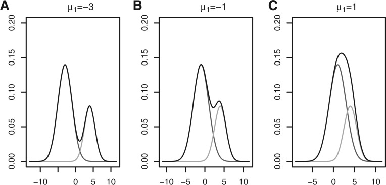
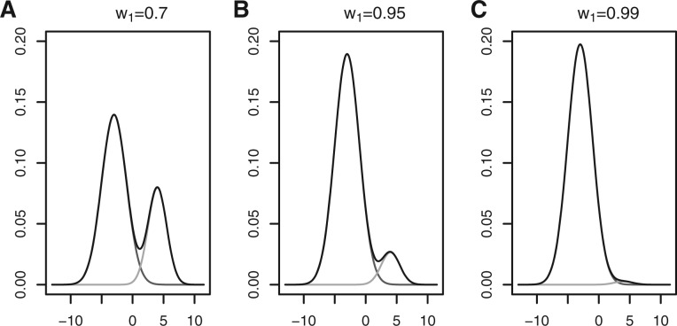
As said in Jain (2010), there is inherent vagueness in the definition of a cluster. We want to illustrate what a cluster is with a toy example. Figure 1 shows a density function of two Gaussian distributions when varying the mean of the first distribution. In Figure 2, the means are fixed, and the proportion for the first Gaussian distribution is varied. Most figures show two distinct peaks. However, we can see that the data should be considered as one cluster in Figures 1C and 2C, because there is only a single peak. An ideal cluster would be such that the corresponding probability density function has a unique peak (mode) and every point can move to the peak following a monotonically nondecreasing path. In this article, we use K-means as a building block to estimate the probability density function (see Sections 2.2 and 2.3), which is then used to partition the clusters based on the above consideration (see Section 2.4).

Fig. 1.

The overall density with two Gaussian mixture components with different choices of mean for the first component. The y-axis for the black curve is the probability density f(x) at x given by the x-axis. The overall density function f(x)=w₁ϕ(x; μ₁, σ₁²)+(1−w₁)ϕ(x; μ₂, σ₂²), where w₁=0.7, μ₂=4, σ₁=2, σ₂=1.5, ϕ(x; μ, σ²) is the density function of the Gaussian distribution with mean μ and variance σ², and μ₁ takes the values of −3, −1, and 1, respectively. The two components w_kϕ(x; μ_k, σ_k²) (k=1, 2) are respectively given by the red and green curves (A color version of this figure is available as Supplementary Material)

Fig. 2.

The overall density with two Gaussian mixture components for different choice of w₁. We set μ₁=−3, μ₂=4, σ₁=2, σ₂=1.5. The presentation of this figure is the same as in Figure 1 except that μ₁ is fixed at -3 and w₁ takes the values of 0.7, 0.95 and 0.99 for the three panels (A color version of this figure is available as Supplementary Material)

2.2 K-means

The K-means algorithm has traditionally been used in unsupervised clustering, and was applied to flow cytometry data as early as in Murphy (1985), and as recently as in Aghaeepour et al. (2011). In fact, K-means is a special case of a Gaussian finite mixture model where the variance matrix of each cluster is restricted to be the identity matrix. Our use of K-means is not for the final clustering, but for a first partition of the cells, for which we can compute the smoothed density function. In the literature, the most popular K-means implementation is based on Lloyd's algorithm (Lloyd, 1982). Since there are many local minima, the final clustering depends critically on the initial seeds. We used the seeds generation algorithm from the K-means++ algorithm (Arthur and Vassilvitskii, 2007). Let x_i=(x_i¹,…, x_i^d) be a d-dimensional vector for the measurements of cell i and c_h be the seed vector for cluster h. Initially, a random cell is picked and assigned to c₁. To sequentially determine the seed for cluster k (k=2,···, K), we first compute the minimum Euclidean distance for all cells to the previous k−1 seeds by

A cell x_i is selected to be the seed c_k of the k-th cluster according to the probability d_i²/{∑_j=1ⁿ d_j²}. After the seeds for all K clusters are assigned, Lloyd's algorithm (Lloyd, 1982) will iterate with the following two steps: assign each data point with a cluster label according to the smallest distance to the K seeds (cluster membership assignment step) and then recompute the center vector of all data points that are assigned with the same cluster label (center update step). The updated center vectors become the seed vectors for the cluster membership assignment step in the next iteration. We use a k-d tree representation of cells (Kanungo et al., 2002) for improved computing speed for the implementation of Lloyd's algorithm. After Lloyd's algorithm converged, we further applied the Hartigan and Wong's (1979) algorithm to recompute the cluster centers and cluster membership to decrease the objective function ∑_i=1ⁿ‖x_i−c_Li‖², where L_i∈1,…, K is the cluster label of x_i and c_k is the center vector for cluster k∈1,…, K. We could have applied the Hartigan and Wong's algorithm directly to the seeds, but the computation is too slow.

In general clustering, it is important to specify a good K in the K-means algorithm. For our purpose, a very accurate specification of K is not necessary. However, it is still important that the K can give a smooth density in which the peaks can reveal the clustering structure. This specification of K is similar to the determination of the number of bins in drawing histograms. We adopted the formula of Freedman and Diaconis (1981)

(1)

where x₍₁₎^j, x_(n)^j are, respectively, the minimum and maximum of the j-th dimension of the data x^j=(x₁^j, x₂^j,…, x_n^j) and IQR(·) is the interquartile range of the data, defined as the difference between the 75th percentile and 25th percentile. Then our K is defined as the median of K_j's, i.e.

(2)

where ⌈·⌉ is the ceiling function that maps a real number to the smallest following integer.

2.3 Gaussian finite mixture to model the density function

After K-means, we may approximate the density function f(x) by the Gaussian finite mixture models,

where the proportion w_k of the k-th component satisfies 0≤w_k≤1 and ∑_k=1^K w_k=1 and ϕ(x; μ_k, Σ_k) is the probability density function of the multivariate normal distribution with mean μ_k and variance matrix Σ_k. After applying the K-means algorithm of Section 2.2, we have already partitioned the data into K clusters, and for the k-th cluster, we can compute the sample proportion w_k, sample mean μ_k and sample variance matrix Σ_k (a rigorous writing would require the hat notation, which is ignored for the sake of simplicity). However, the estimate Σ_k may be too noisy, and we want to smooth the variance matrix by

where h and h₀ are customized parameters tuned to make the density function smoother or rougher. The default setting in the software is h=1.5 and h₀=1. Here, λ_k=nw_k/(k+nw_k) so that a greater w_k results in a λ_k closer to 1; Σ₀ is the variance matrix assuming the data are uniformly distributed in the whole data range and is a diagonal matrix with its (j, j) element Σ₀^j,j={(x_(n)^j−x₍₁₎^j)/k^1/d}² for j=1,…, d.

2.4 Peak search and merging

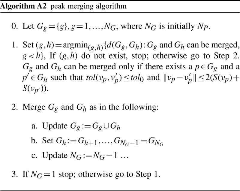
According to our definition, a cluster is defined by the local peak. For all cells, we can use the greatest gradient search (hill climbing) to find which local peak a given cell can reach. This rules out any global optimization strategy such as the conjugate gradient algorithm. It is computationally very time consuming to search all the local maximums of the density function for all cells. Since the cells are pre-grouped by the K-means, we only need to search the local peaks for the centers of the K-means clusters. The hill climbing method searches along the greatest gradient of the density function. If we take the negative of the density function as the optimization function, the hill climbing of peak search can be achieved by the deepest descent algorithm, which is implemented by the GSL library at http://www.gnu.org/software/gsl/. We also need to restrict the step size in case it steps too far away and jumps to another local peak. When the data move from one K-means cluster into another K-means cluster, we can speed it up by moving directly to the center of the other cluster. When two peaks are relatively close, they should be joined together and considered as a single peak. We search the two peaks with the closest Euclidean distance and check if the two clusters may not be too different from a single cluster. The details on the local peak search and peak merging are described in the Appendix. Algorithm 1 gives the summary of the steps to use in K-means and density peak finding in order to cluster the flow cytometry data as implemented in the software flowPeaks. In the end, we will obtain (≤K) of merged clusters, each of which consists of one or many K-means clusters.

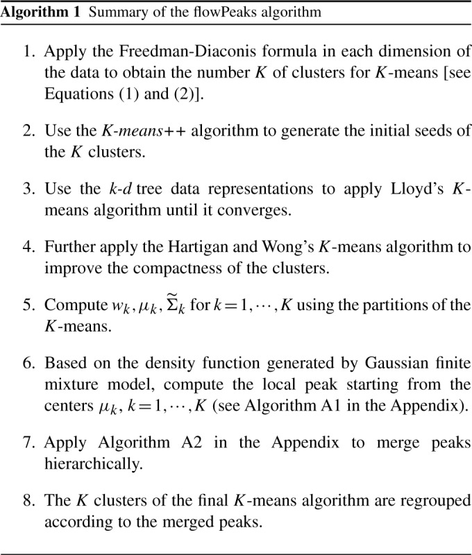
2.5 Cluster tightening

The default setting in the flowPeaks algorithm is to not identify the outliers. Some data points may lie far from the center or cannot be unambiguously classified into a specific cluster. We determine whether a data point is an outlier using the following strategy. Let ℓ(x) be the final merged cluster label of data point x. Let ω_i and f_i(x) (respectively) be the proportion and the probability density function of the i-th final merged cluster. The proportion ω_i is the sum of w_k's of the K-means clusters that form the i-th final merged cluster. The density function f_i(x) itself is a Gaussian finite mixture based on the K-means clusters that are merged into the i-th final cluster, while the overall density function f(x) is based on all K-means clusters (see Section 2.3) and f(x)=∑_i=1 ω_if_i(x). A point x is an outlier if

or

The numbers 0.01 and 0.8 can be adjusted in the software settings.

3 RESULTS

3.1 Datasets

Barcode data: The data were generated for a barcoding experiment (Krutzik and Nolan, 2006) with varying concentrations of flurophores (APC and Pacific Blue). The flow cytometry data have 180912 cells and three channels with an additional channel for Alexa. The manual gates for the 20 clusters to be used for assessing cluster algorithm performance were created from flowJo (www.flowjo.com).

Simulated concave data: The data were simulated with two distinctive concave shapes based on the idea from the supplemental material of Pyne et al. (2009). It has 2729 rows and 2 columns. Both barcode data and simulated concave data along with their gold standard cluster labels are available in the flowPeaks package.

GvHD dataset: Graft versus host disease dataset and the manual gates are obtained from Aghaeepour et al. (2011). This dataset contains 12 samples, and the cells are stained with four markers, CD4, CD8b, CD3 and CD8. In addition, two channels FS and SS are also measured. These data are mostly analyzed based on the four markers unless specified otherwise. The numbers of cells of the 12 samples range from 12 000 to 32 000.

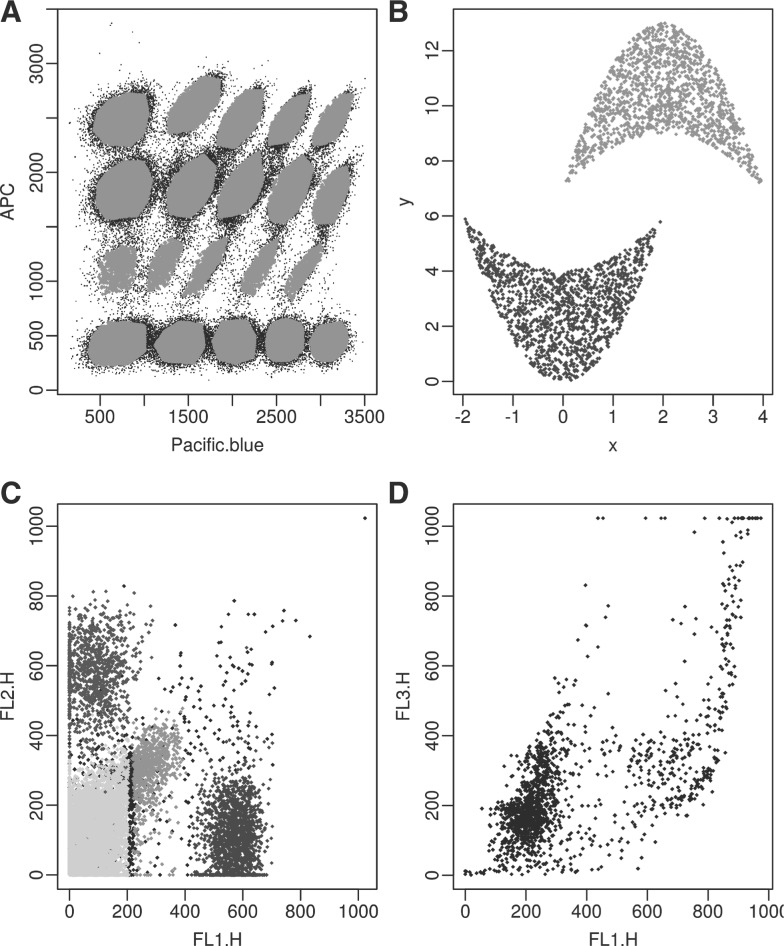
Rituximab data: The flow cytometry data that are obtained from the flowClust package (Lo et al., 2009). They have 1545 cells and two channels of interest. The data were originally produced by Gasparetto et al. (2004). The barcode data, simulated data and GvHD datasets have gold standard cluster labels (either by simulation or manual gating) to assess performance. The rituximab data are used for the purpose of exploration. Figure 3 displays all four datasets.

Fig. 3.

Four example datasets: (A) barcode data with the 20 clusters. (B) Concave data with two clusters. (C) One of the 12 samples in the GvHD dataset. The plot only shows the scatter plot of the first two of the four channels, where different colors indicate different manual gated clusters and black points are outliers. (D) Rituximab data (A color version of this figure is available as Supplementary Material)

3.2 Different metrics to assess the cluster algorithm performance

The most widely used metric to assess how a candidate clustering algorithm compares with the gold standard, for which the correct cluster membership is known, is the adjusted Rand index (Hubert and Arabie, 1983; Rand, 1971). The Rand index (Rand, 1971) is based on the percentage of the agreement between the two clustering methods. Let us assume that n data points are labeled differently with two different clustering methods, say Method A and Method B with K_A and K_B clusters. Let A_i,i=1,…, n and B_i,i=1,…, n be the cluster labels for the two methods. The Rand index is defined as

where I(·) is the indicator function. The adjusted Rand corrects for chance, and the general form is

In order to compute the adjusted Rand index, we first define the contingency tables

for a=1,…, K_A, b=1,···, K_B. The marginal sums on the contingency tables are then defined as

Note that n=∑_a=1^K_An_a,+=∑_b=1^K_B n_+,b. The adjusted Rand index can be quickly computed using the following formula (Hubert and Arabie, 1983)

The F-measure (Fung et al., 2003) is based on a greedy strategy to match the two clustering. It has been used in 2010s flowCAP I (http://flowcap.flowsite.org/summit2010.html) and in the flowMeans algorithm paper (Aghaeepour et al., 2011) to assess the performance of different algorithms. The F-measure is defined as

where .

Rosenberg and Hirschberg (2007) proposed the V-measure to evaluate the clustering algorithm. This measure uses entropy to assess how much a second clustering provides extra information for the first clustering. For the clustering Method A, the entropy is

and the conditional entropy

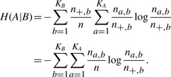The conditional entropy H(A|B) is always no greater than the entropy H(A). The extra information provided by Method B for Method A is the reduced entropy H(A)−H(A|B). After normalization, we can define

In the above equation, by definition h=1 if H(A)=0. If we reverse the positions of A and B, we can define

If Method B is the candidate clustering to be compared with the gold standard clustering A, h evaluates the homogeneity of clustering for Method B, while c evaluates the completeness. The homogeneity ensures that the gold standard labels (A labels) for all data points of a candidate cluster B are unique. Completeness ensures that for each gold standard cluster (A cluster), data points are all assigned to a single candidate cluster (B cluster). Details can be found in Rosenberg and Hirschberg (2007). The V-measure is a weighed harmonic mean of h and c, V_β=(1+β)hc/(βh+c). In this artice, we will fix β to be 1.

3.3 Application

Table 1 displays the running time of all algorithms that are applied to the concave and barcode datasets described in Section 3.1. The algorithms flowPeaks, Misty Mountain (Sugar and Sealfon, 2010), FLOCK (Qian et al., 2010) and flowMeans (Aghaeepour et al., 2011) are falling into a category where the computational time is under several minutes so that they can compete with manual gating, while FLAME (Pyne et al., 2009) and flowMerge (Finak et al., 2009) take too much computational time to be practically useful. Among the first four algorithms, a good seeding strategy and k-d tree implementation make flowPeaks a little bit faster than the other algorithms.

Table 1.

Comparison of the running time of different flow cytometry clustering algorithms

	flowPeaks	Misty mountain	FLOCK	flowMeans	FLAME	flowMerge
Concave	0.13	0.59	6	6.2	1434	3202
Barcode	2.3	24.7	14	82.3	80 952	132 446

The running time is shown in wall-clock seconds on the same desktop computer except that FLOCK and FLAME were run, respectively, at immport (http://immport.niaid.nih.gov) and gene pattern websites (http:www.broadinstitute.org/cancer/software/genepattern)

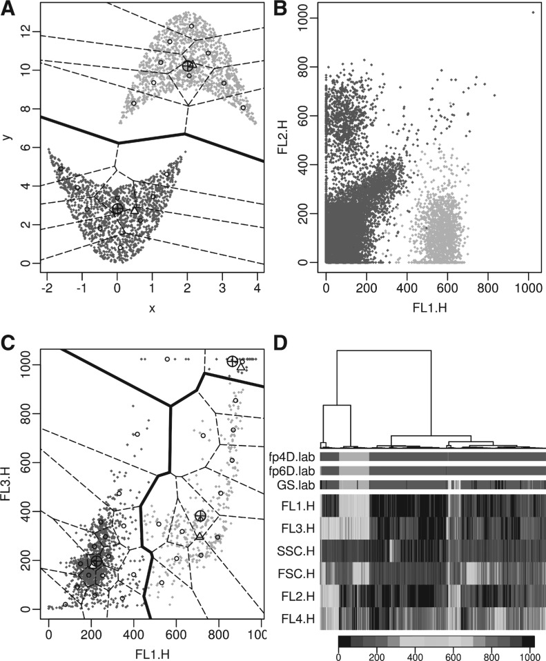
When we applied the three metrics in Section 3.2 to assess different algorithms, we removed the outliers according to the gold standard. Tables 2 and 3 give the performance of different algorithms to be compared with the gold standard. We see that flowPeaks does quite well for the barcode data and the concave data. Due to the slow speed of flowMerge and FLAME and the difficulty to batch running FLOCK and FLAME, which are only available from a web interface, for performance comparison on the 12 samples in the GvHD dataset, we only selected flowPeaks, Misty Mountain and flowMeans, which are the three best algorithms according to Tables 2 and 3. Table 4 shows that flowPeaks is better than the other two algorithms for the GvHD dataset. We have displayed the flowPeaks results for the four datasets in Figures 4A, 5A–C. Since rituximab does not have a gold standard, the visual display shows that flowPeaks does a good job revealing the cluster structure of the data. Figure 5D displays the application of flowPeaks in the GvHD data when FSC and SSC channels are included. The clustering on 6D highly agrees with 4D with only 0.59% of points classified differently between 6D and 4D.

Table 2.

The performance of different algorithms on the barcode data

	flowPeaks	Misty mountain	FLOCK	flowMeans	FLAME	flowMerge
Adj-Rand	0.998	0.971	0.258	0.998	0.859	0.801
F-measure	0.993	0.984	0.341	0.993	0.868	0.887
V-measure	0.996	0.967	0.567	0.995	0.946	0.952

Adj-Rand is for the adjusted Rand index.

Table 3.

Performance of different algorithms on the concave data

	flowPeaks	Misty mountain	FLOCK	flowMeans	FLAME	flowMerge
Adj-Rand	1.000	1.000	0.501	0.723	0.232	0.952
F-measure	1.000	1.000	0.683	0.884	0.438	0.987
V-measure	1.000	1.000	0.667	0.713	0.480	0.932

Adj-Rand is for the adjusted Rand index.

Table 4.

The comparison of the performance on the 12 samples of the GvHD dataset

	flowPeaks	Misty mountain	flowMeans
Adj-Rand	0.807 (0.175)	0.675 (0.287)	0.573 (0.292)
F-measure	0.924 (0.075)	0.859 (0.146)	0.848 (0.120)
V-measure	0.816 (0.135)	0.664 (0.205)	0.639 (0.199)

Adj-Rand is for the adjusted Rand index. Each entry lists the mean and standard deviation.

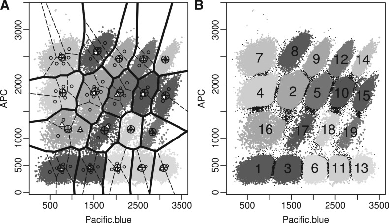
Fig. 4.

Application of flowPeaks to the barcode data. (A) the bold boundary displays the clusters output by flowPeaks with their centers (⊕), the dotted lines are the boundary for the underlying K-means clusters with their centers (○). The local peaks are indicated by ▵. (B) The same as in (A) except the outliers have been identified as black points and other secondary information was not displayed, and the clusters are labeled according to their proportions (w_k) (A color version of this figure is available as Supplementary Material)

Fig. 5.

The application of flowPeaks to different datasets. See Figure 4A for explanations of legends. (A) Concave data. (B) One sample of the GvHD dataset that is shown in Figure 3C. The boundaries between flowPeaks clusters and between K-means clusters are not drawn as two non-overlapping clusters generated in 4D may overlap in a 2D projection. (C) Rituximab dataset. (D) The same sample in (B) with FSC and SSC channels included. Due to the long running time required for the heatmap, 4000 data points were randomly selected to generate the cluster-tree and the heatmap. The three rows fp4D.lab, fp6D.lab and GS.lab, respectively, display the class labels of the flowPeaks on 4D, flowPeaks on 6D, and the Gold Standard, where different colors indicate different clusters. The signal intensities of all six channels are displayed in the heatmap with the key displayed on the bottom (A color version of this figure is available as Supplementary Material)

4 SOFTWARE

We have implemented the algorithm in C++ wrapped into an R package named ‘flowPeaks’. The following example illustrates how to use the basic functions of this R package

The above R script will display Figure 4A. In order to identify the outliers to obtain Figure 4B, we can proceed further with the following script

For further use of the software flowPeaks, one can consult the package's vignette pdf file and help documents.

5 DISCUSSION AND FUTURE WORK

In this article, we described the algorithm flowPeaks that combines the K−means and density function peak finding to partition the flow cytometry data into distinct clusters. We have compared our algorithm with other state of the art algorithms for real and simulated datasets. Our algorithm is fast and able to detect the non−convex shapes. We should point out that flowPeaks's goal is to find the overall density shape and search for global structure. It will not be able to uncover overlapping clusters as shown in Figure 1C or the rare cluster as shown in Figure 2C. The flowPeaks algorithm is based on the geometrical shape of the density function. Prior to apply flowPeaks, data transformation may be necessary to reveal the structure, and irrelevant channels need to be first discarded to avoid the curse of dimensionality. Due to the curse of dimensionality, if the data dimension is too high and the number of cells is too low where the density function cannot be reliably estimated by flowPeaks, users should alternatively use the heatmap to visualize the data.

As commented in Jain (2010), there is not a single clustering algorithm suitable for all datasets. This is probably true for flow cytometry clustering. There is not a good collection of flow cytometry data with gold standard gates, which makes algorithm comparison very challenging. The comparison in Section 3.3 should not be taken literally. We tend to agree with Naumann et al. (2010) that ‘it is too early for extensive comparisons of automated gating procedure’. The current approach of using the manual gating as a gold standard to compare the automatic gating algorithm is very subjective. We participated with flowPeaks and support vector machine algorithm in 2011's flowCAP II (http://flowcap.flowsite.org/summit2011.html). Our algorithm gave 100% prediction accuracy for the clinical flow cytometry data, establishing us as one of the best algorithms. We have released our datasets in our flowPeaks package with the gold standard gates so that one can test one's favorite algorithm with our datasets. The source code and windows binary built of the R package flowPeaks is available at https://github.com/yongchao/flowPeaks. The package is in the progress of being permanently hosted at the Bioconductor (Ihaka and Gentleman, 1996; Gentleman et al., 2004) with open source code for algorithm developers and batching processing.

APPENDIX

Mathematical notation

For the sake of clarity, we will use the following notation. Assume the data consist of n points in d dimension.

Let the underlying clusters, obtained by K−means, be labeled as 1,…, K. The density function generated by the finite mixture model is

where w_k, μ_k, are the weights, means and the smoothed variance matrix of cluster k, respectively, for k = 1,…, K. The derivative of the density function at x is defined as

According to the K-means algorithm, the cluster label of x can be defined as

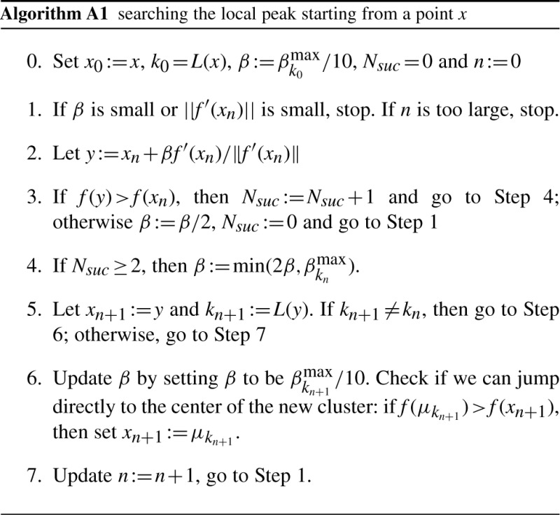
Searching the local peak starting from a point x

As we do not want to jump over the local peak, when the data fall into a cluster k, we define the maximum step size

The detailed computations for the local peak search are described in Algorithm A1. We initially set a small step size β (Step 0), and try to find a step size such that the density function f improves (Step 2 and Step 3). If the same step size improves twice in a row (N_suc denote the number of continuous improvements), then we double the step size; otherwise we half the step size. If the point is falling into a new cluster, we want to find out if we can jump to the new center directly (Step 6). The details are described in Algorithm A1.

The algorithm on merging local peaks

When two peaks are close and the density function between the two peaks is relatively flat, the two peaks should be combined into one. For each underlying K−means cluster, we define the nearest neighbor cluster distance by

For an arbitrary position x, we can similarly define the function S(x) = S_L(x). Let x and y be two points, we define the tolerance that describes how the density function of the line segment that connects x and y can be approximated by a straight line

where z_t=x+t(y-x) and . The function is the fitted density function at the position z_t by using a straight line to connect the two points (x, f(x) and (y, f(y)). The second term in defining tol corrects for cluster sample sizes.

Many K-means centers may reach the same local peak. A local peak can then be represented by a subset P_j of {1,…, K} and its location is denoted by ν_j, where j=1,…, N_P and N_P is the number of distinct local peaks. In other words, for each k in P_j, μ_k will move to the same ν_j by using our local peak algorithm. Initially, set G_g={g}, g=1,…, N_P, i.e. each peak set just contains a single peak (Step 0). Two peak sets can be merged only if the two peaks are relative close and the density function between the peaks is relatively flat (Step 1). G_g are merged hierarchically (Step 2). The details are given in Algorithm A2. After the algorithm completes, N_G is the number of (see Section 2.4) final clusters.

REFERENCES

- Aghaeepour N., et al. Rapid cell population identification in flow cytometry data. Cytometry A. 2011;79:6–13. doi: 10.1002/cyto.a.21007. [DOI] [PMC free article] [PubMed] [Google Scholar]
- Arthur D., Vassilvitskii S. Proceedings of the Eighteenth Annual ACM−SIAM Symposium on Discrete Algorithms. New Orleans: SIAM; 2007. k-means++: the advantages of careful seeding; pp. 1027–1035. [Google Scholar]
- Chan C., et al. Statistical mixture modeling for cell subtype identification in flow cytometry. Cytometry A. 2008;73:693–701. doi: 10.1002/cyto.a.20583. [DOI] [PMC free article] [PubMed] [Google Scholar]
- Finak G., et al. Merging mixture components for cell population identification in flow cytometry. Adv. Bioinformatics. 2009;2009:247646. doi: 10.1155/2009/247646. [DOI] [PMC free article] [PubMed] [Google Scholar]
- Freedman D., Diaconis P. On the histogram as a density estimator: L2 theory. Zeitschrift fur Wahrscheinlichkeitstheorie und verwandte Gebiete. 1981;57:453–476. [Google Scholar]
- Fung B.C.M., et al. Proceedings of the Third SIAM International Conference on Data Mining (SDM) San Francisco, CA: SIAM; 2003. Hierarchical document clustering using frequent itemsets; pp. 59–70. [Google Scholar]
- Gasparetto M., et al. Identification of compounds that enhance the anti-lymphoma activity of rituximab using flow cytometric high-content screening. J. Immunol. Methods. 2004;292:59–71. doi: 10.1016/j.jim.2004.06.003. [DOI] [PubMed] [Google Scholar]
- Gentleman R., et al. Bioconductor: open software development for computational biology and bioinformatics. Genome Biol. 2004;5:R80. doi: 10.1186/gb-2004-5-10-r80. [DOI] [PMC free article] [PubMed] [Google Scholar]
- Hartigan J.A., Wong M.A. A K-means clustering algorithm. Appl. Stat. 1979;28:100–108. [Google Scholar]
- Hubert L., Arabie P. Comparing partitions. J. Classif. 1983;2:193–218. [Google Scholar]
- Ihaka R., Gentleman R. R: a language for data analysis and graphics. J. Comput. Graph. Stat. 1996;5:299–314. [Google Scholar]
- Jain A.K. Data clustering: 50 years beyond K-means. Pattern Recogn. Lett. 2010;31:651–666. [Google Scholar]
- Kanungo T., et al. An efficient k-means clustering algorithm: analysis and implementation. IEEE Trans. Pattern Anal. 2002;24:881–892. [Google Scholar]
- Krutzik P., Nolan G. Fluorescent cell barcoding in flow cytometry allows high-throughput drug screening and signaling profiling. Nat. Methods. 2006;3:361–368. doi: 10.1038/nmeth872. [DOI] [PubMed] [Google Scholar]
- Lloyd S.P. Least squares quantization in PCM. IEEE Trans. Inform. Theory. 1982;IT-28:129–139. [Google Scholar]
- Lo K., et al. Automated gating of flow cytometry data via robust model-based clustering. Cytometry A. 2008;73:321–32. doi: 10.1002/cyto.a.20531. [DOI] [PubMed] [Google Scholar]
- Lo K., et al. flowClust: a Bioconductor package for automated gating of flow cytometry data. BMC Bioinformatics. 2009;14:145. doi: 10.1186/1471-2105-10-145. [DOI] [PMC free article] [PubMed] [Google Scholar]
- Murphy R.F. Automated identification of subpopulations in flow cytometric list mode data using cluster analysis. Cytometry. 1985;6:302–309. doi: 10.1002/cyto.990060405. [DOI] [PubMed] [Google Scholar]
- Naumann U., et al. The curvHDR method for gating flow cytometry samples. BMC Bioinformatics. 2010;11:44. doi: 10.1186/1471-2105-11-44. [DOI] [PMC free article] [PubMed] [Google Scholar]
- Pyne S., et al. Automated high-dimensional flow cytometric data analysis. Proc. Natl. Acad. Sci. USA. 2009;106:8519–8524. doi: 10.1073/pnas.0903028106. [DOI] [PMC free article] [PubMed] [Google Scholar]
- Qian Y., et al. Elucidation of seventeen human peripheral blood B-cell subsets and quantification of the tetanus response using a density-based method for the automated identification of cell populations in multidimensional flow cytometry data. Cytometry B. 2010;78:S69–S82. doi: 10.1002/cyto.b.20554. [DOI] [PMC free article] [PubMed] [Google Scholar]
- Rand W.M. Objective criteria for the evaluation of clustering methods. J. Am. Stat. Assoc. 1971;66:846–850. [Google Scholar]
- Rosenberg A., Hirschberg J. Proceedings of the 2007 Joint Conference on Empirical Methods in Natural Language Processing and Computational Natural Language Learning. Prague: Association for Computational Lingusistics; 2007. V-Mmeasure: a conditional entropy-based external cluster evaluation measure; pp. 410–420. [Google Scholar]
- Sugar I.P., Sealfon S.C. Misty Mountain clustering: application to fast unsupervised flow cytometry gating. BMC Bioinformatics. 2010;11:502. doi: 10.1186/1471-2105-11-502. [DOI] [PMC free article] [PubMed] [Google Scholar]