

Abstract
Motivation: Protein abundance in quantitative proteomics is often based on observed spectral features derived from liquid chromatography mass spectrometry (LC-MS) or LC-MS/MS experiments. Peak intensities are largely non–normal in distribution. Furthermore, LC-MS-based proteomics data frequently have large proportions of missing peak intensities due to censoring mechanisms on low-abundance spectral features. Recognizing that the observed peak intensities detected with the LC-MS method are all positive, skewed and often left-censored, we propose using survival methodology to carry out differential expression analysis of proteins. Various standard statistical techniques including non-parametric tests such as the Kolmogorov–Smirnov and Wilcoxon–Mann–Whitney rank sum tests, and the parametric survival model and accelerated failure time-model with log-normal, log-logistic and Weibull distributions were used to detect any differentially expressed proteins. The statistical operating characteristics of each method are explored using both real and simulated datasets.
Results: Survival methods generally have greater statistical power than standard differential expression methods when the proportion of missing protein level data is 5% or more. In particular, the AFT models we consider consistently achieve greater statistical power than standard testing procedures, with the discrepancy widening with increasing missingness in the proportions.
Availability: The testing procedures discussed in this article can all be performed using readily available software such as R. The R codes are provided as supplemental materials.
Contact: ctekwe@stat.tamu.edu
1 INTRODUCTION
Proteomics is a growing field that deals with the determination of gene and cellular function at the protein level (Aebersold and Mann, 2003). It is often of interest to the protein researcher to identify as well as quantify the amount of protein in a given biological sample. Several methods and instruments are available for both the identification and quantitation of peptides within proteins, including the bottom-up liquid chromatography mass spectrometry (LC-MS) and LC-MS/MS or the tandem mass spectrometry approaches. In the LC-MS approach, proteins are extracted from the biological sample, digested into peptides and ionized (Karpievitch et al., 2010; Vogel and Marcotte, 2008). Following the ionization step, the ionized sample is introduced to the mass spectrometer for scanning where the mass to charge (m/z) and observed peak intensities are obtained. Once the peak intensities are obtained, the observed features of the peptides are matched to a database for peptide identification. Following the identification step, the peptide level information is rolled up to the protein level (Karpievitch et al., 2010). In LC-MS/MS, a precursor ion is picked after the first MS step for fragmentation prior to the identification step (Karpievitch et al., 2010). It is often of interest to measure the abundance of proteins from the identified peptides in the sample; this is the quantitation step of the analysis.
In bottom-up MS-based quantitation, the estimation of protein abundances in a sample is typically carried out on the basis of one of three quantities (Hendrickson et al., 2006; Karpievitch et al., 2010; Zhu et al., 2009): (i) spectral counts; (ii) label-free methods or (iii) isotopic labeling experiments. Spectral counts are simply the number of peak intensities for a given peptide/protein. Label-free intensity-based quantitation uses peak intensities (heights or areas under the peaks) to estimate peptide or protein abundance. Other label-free methods are based on the unlabeled peak intensities associated with the mass spectrum of the extracted ions. Label-based methods of quantitation, which are viewed as the ‘gold-standard’ for measuring protein abundance, involve the ratio of the observed peak intensities of two isotopically labeled samples. Once the protein abundances have been obtained, it is often of interest to assess differentially expressed proteins across comparison groups. The goal of differential analysis is to differentiate features across groups which can be subsequently used for biomarker discovery or for providing additional clues for studying the causal pathways of the disease or the biological condition of interest (deVera et al., 2006).
One of the characteristics of peak intensity data from LC-MS based proteomics is large quantities of missing data. The missing data patterns are often not independent of the peak intensities of the peptides, which is likely due to censoring of the peak intensities for low-abundance peptides/proteins (Karpievitch et al., 2009). To assess differentially expressed proteins across treatment groups, the observed peak intensities are often normalized (Callister et al., 2006), imputed (Jornsten et al., 2005; Troyanskaya et al., 2001) and transformed (Cui and Churchill, 2008; Thygeson and Zwinderman, 2004). Various imputation techniques are available for the imputation step. These include the row mean imputation, K nearest neighbor (KNN) (Troyanskaya et al., 2001), singular value decomposition (Troyanskaya et al., 2001), Bayesian principal components analysis (Oba et al., 2003), Gaussian mixture clustering (Ouyang et al., 2004) and a convex combination of these methods (LinCmb) (Jornsten et al., 2005). Another imputation approach is the probabilistic PCA (PPCA) approach which is based on a combination of the expectation maximization (EM) algorithm with a probability model (Stacklies et al., 2007). Once the data are transformed and imputed, standard statistical techniques such as the two-sample t-tests or linear regression methods are often applied to detect any significant differences in the protein expressions across the groups under the assumption that the data are normally distributed. However, the assumption of normality can be violated even for the transformed data. The protein-specific t-test may also have insufficient power in detecting group differences due to the small sample sizes within each treatment group (Cui and Churchill, 2003).
To deal with missing values in practice, one of two basic strategies is generally used. The simplest strategy is to work only with the complete intensities. That is the data used for a particular peptide/protein would be based on the observed peak intensity; the missing values are excluded from the analysis. Alternatively, the missing values are imputed. There are many imputation algorithms (Jornsten et al., 2005; Oba et al., 2003; Ouyang et al., 2004; Stacklies et al., 2007; Troyanskaya et al., 2001). However, none of these approaches is strictly appropriate when the missing values have been censored, as they can result in biased estimates and statistical inference (Karpievitch et al., 2009).
Standard alternatives to the parametric t-test are non-parametric tests such as the Wilcoxon–Mann–Whitney rank sum or the Kolmogorov–Smirnov tests. These tests are more desirable than their parametric counterpart since they do not make any strong distributional assumptions. As with the t-test, these tests are carried out by either deleting the missing peak intensities or imputing the data. Standard statistical techniques such as the t-test or linear regression methods do not naturally accommodate the positive nature of the data, nor the presence of widespread censoring.
To address these issues, we propose the use of existing statistical methodology that is designed specifically for non-negative, censored data. The field of survival analysis generally deals with such data, and there is a wide variety of survival methodologies that could be adapted to the quantitative proteomics setting. In particular, the accelerated failure time (AFT) model fits the quantitative proteomics setting well. An AFT model essentially; involves regression under assumed parametric models, in the presence of censored observations. Distributions available in AFT modeling include the log-normal, log-logistic and Weibull.
As discussed above, standard testing procedures in the quantitative proteomics setting are not ideal, particularly with regard to the widespread censoring that is typically present. A simple scenario highlights the value of survival methods in the presence of censored data. Consider a single protein for which we have intensity measurements from 10 control samples and 10 treatment samples. Of the 20 attempted measurements, suppose 6 are missing due to censoring: 2 from the control group and 4 from the treatment group. For these six censored observations, we can only say that the protein was not present for those samples, or it peak intensities were too low to be detected by the instrument. In our data file, the entries for these 6 observations might simply read ‘NA.’ The challenge is dealing with this situation that the 14 observed intensities will tend to the 14 ‘largest’ values out of the 20. Thus, for example, if we were to base our analysis on just the 14 observed intensities, we would ‘overestimate’ the means and ‘underestimate’ the standard deviations in each group, resulting in biased inference. Meanwhile, standard imputation routines assume that missing values are ‘completely at random’ (Little and Rubin, 2002), which in our context would mean that the fact a particular intensity is missing is independent of the value of its actual peak intensity or other peak intensities in the data. With censoring, observations tend to go missing only when they are really small (in our left censoring contexts). In other words, the missing completely at random mechanism does not generally apply to quantitative proteomics data. As such, standard imputation techniques will suffer from the same limitations of the complete-data analysis, namely, biased statistical inference.
Furthermore, most imputation techniques that are applied in practice to quantitative proteomics data are ‘single imputation’ techniques (Little and Rubin, 2002). It is known that single imputation can result in biased inference due to overfitting the data. Survival methodology, of which AFT models are an example, is specifically designed to handle censored observations. They work by correctly representing a censored observation as one that in reality fell at or below a known threshold. As a result, the issues of overestimated group means and underestimated standard deviations are avoided, and valid statistical inference is maintained. The main contribution of this article is to adapt well-known benefits of survival methodology to the quantiative proteomics setting. Our proposed approach to detecting differential expressions can be applied to any proteomics data generated using either the LC-MS or tandem MS approaches since these data are all non-negative and prone to missing observations due to censoring regardless of the instrument technology. The advantage of using the survival approach is that it allows a likelihood-based inference of the LC-MS or LC-MS/MS proteomics data in the presence of missingness due to censored observations.
2 METHODS
2.1 Data preprocessing
One of the challenges in proteomic analysis is determining how the peptide level information obtained for each peak height can be rolled up to the protein level. Analysis conducted at the peptide level for each protein is often desirable; however, such analysis is not always feasible due to the level of missing data at the peptide-level. In a peptide-level analysis, the protein-level abundance is expressed in terms of the peptide-level intensities, and methods such as mixed effects models are used in the analysis (Karpievitch et al., 2009). Several options are available for the peptide to protein rollup in LC-MS-based bottom-up proteomics. These options include the RRollup, ZRollup and QRollup (Polpitiya et al., 2008). In the RRollup method, all peptides from a given protein are scaled based on a reference peptide and averaged to obtain a protein abundance for that given protein (Polpitiya et al., 2008). The ZRollup method involves standardizing at the peptide level using a method comparable to the z-scores prior to averaging to obtain the protein-level abundance (Polpitiya et al., 2008). For the QRollup method, a user specified cutoff value is used to select the peptides for a given protein, and the selected peptides are averaged across peptide-level peak intensities to obtain protein-level abundances (Polpitiya et al., 2008). Another approach to the peptide to protein rollup problem is a principal components based approach (ProPCA) for label-free LC-MS/MS proteomics data (Dicker et al., 2010). The ProPCA method combines the spectral counts from the label-free LC-MS/MS data with the peptide peak attributes to obtain estimates of the relative protein abundance (Dicker et al., 2010).
For simplicity, we accomplished peptide-to-protein rollup by averaging peptide peak intensities by protein. In addition to the AFT models, we considered the following strategies for dealing with missing intensities at the protein level: (i) complete data analysis, row-mean imputation, KNN imputation (Troyanskaya et al., 2001), and PPCA imputation (Stacklies et al., 2007). As discussed above, these and related techniques, while simple to implement in practice, have important limitation in the quantitative proteomics setting that can result in invalid statistical inference.
2.2 Data
2.2.1 Diabetes study
For our first application, we apply the various tests to the diabetes data studied by (Karpievitch et al., 2009). The diabetes dataset is based on frozen human serum samples from the DASP between 2000 and 2009 (Metz et al., 2008). The data consist of 10 healthy control subjects and 10 subjects with a recent diagnosis of type I diabetes mellitus. Six high-abundant plasma proteins that constitute ~85% of the total protein mass of human plasma were removed prior to extracting the serum. The samples were analyzed using the accurate mass and tag method (Pasa-Tolic et al., 2004; Zimmer et al., 2006). The final LC-FTICR MS datasets were processed using the PRISM Data Analysis system (Kiebel et al., 2006). For the diabetes data, any observations within a given sample below the lowest observable peak intensity within that sample is considered censored. Therefore, we define the detection limit to be sample specific for the diabetes data.
2.2.2 Simulation study
We simulated 100 datasets from the log-normal, Weibull and log-logistic distributions. Each simulated dataset was composed of 10 samples in each of two comparison groups with 5000 proteins, 40% of which were differentially expressed. Differential expression was created in terms of differences in log means between the two comparison groups; this difference was allowed to vary from 1.05 to 1.50. We varied the percent missing (censored) observations over the values 0, 5, 15, 25, 35, and 45%. Five approaches were used to handle the censored data. The approaches include no imputation (NI), row mean, KNN and PPCA imputations. We also considered the missing data as left-censored observations by applying survival models. The knn.impute function in the impute package in R (Troyanskaya et al., 2001) with k=3 nearest neighbors was used for the KNN imputation, while the pca function of the pcaMethods package (Stacklies et al., 2007) was used to impute the data with the PPCA approach. The detection limit for our simulation study is defined as the minimum observable peak intensity within the whole dataset. Therefore, the detection limit is data specific for the simulation study.
2.3 Statistical methods considered
2.3.1 T-tests and related techniques
The standard statistical technique used for differential expression analysis in a two-class setting is the two-sample t-test. Under the assumption that the variances are equal for both treatment groups within a given protein and the sampled from a normal population, the data are log2 transformed and the following test statistic
| (1) |
is calculated where Sp is the pooled standard deviation, while C and D index the first and second comparison groups, respectively; M is the total number of proteins in the data and n is the total number of samples associated with each protein. It is assumed that under the null hypothesis, TSi follows a t distribution with 2n−2 degrees of freedom. When the number of comparison groups exceeds two, the two-sample t-test can be generalized by the F-test.
2.3.2 Non-parametric alternatives
Two non-parametric methods were considered for testing the null hypothesis that the distributions of the comparison groups are identical. Non-parametric tests are performed under mild distributional assumptions regarding the distribution of the populations from which the data are sampled (Hollander and Wolfe, 1999). It has been shown that by relaxing the normality assumption when the normality assumption holds in favor of non-parametric methods, the non-parametric methods are minimally less efficient than standard methods based on normality assumptions (Hollander and Wolfe, 1999). Also, the non-parametric tests are more robust to outlying observations even when the normality assumption is valid (Hollander and Wolfe, 1999).
The first distribution-free method we considered was the Kolmogorov–Smirnov test. This tests the null hypothesis that the distributions for the two comparison groups are equivalent against the alternative hypothesis that they differ (Hollander and Wolfe, 1999). Let Fi(·) and Gi(·) be continuous distributions for the populations being compared for the ith protein, and 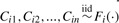 ; and
; and 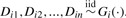 . Our objective is to test if there are any differences in the protein expressions between the two groups. The hypotheses under consideration are
where t is the observed peak intensity. The first step in obtaining the Kolmogorov–Smirnov test statistic is to calculate the empirical distributions of Fin(t) and Gin(t),
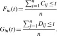 |
The Kolmogorov–Smirnov test statistic Ji for the ith protein is defined as
| (2) |
where d is the greatest common divisor of n. To test at level α, we compare Ji to jα, rejecting the null hypothesis if Ji≥jα. The above test statistic was calculated under the assumption that there are equal samples in both groups; however, the test can also be generalized to the unequal sample size case (Hollander and Wolfe, 1999). The term jα is chosen from a table or computed through software such that the probability of Type I error is equal to α.
The Wilcoxon–Mann–Whitney rank-sum test is a distribution-free two-sample test under the assumption that the populations only differ by location and are independent (Hollander and Wolfe, 1999). A location-shift model defined as Gi(t)=Fi(t−▵i) for every t is used to define the null hypothesis. Under the null, it is assumed that the comparison groups come from identical populations, for the ith protein. The alternative hypothesis is that the two distributions differ by ▵i for the ith protein. More formally,  which states that the distribution of Di and Ci differ by ▵i, the location-shift parameter or treatment effect. Thus, the Wilcoxon–Mann–Whitney hypothesis is stated as
The Wilcoxon–Mann–Whitney rank-sum test statistic, Wi, is computed by first combining the comparison groups (each of size n). The combined sample of size 2n observations is ranked and the test statistic for the ith protein is based on the sum of the ranks assigned to the observations from one of the comparison groups in the ordered combined group. Thus, Wi is calculated as
| (3) |
where Sij is the rank associated with the jth sample from one selected comparison group treatment sample for the ith protein. For this two-sided test, Wi is rejected if Wi≥ωα/2 or if Wi≤n(2n+1)−ωα/2 where the nominal values of ωα/2 can be found through software. Ties are treated separately (Hollander and Wolfe, 1999). Similar to the two-sample t-test, a limitation of the non-parametric tests considered here is that they are restricted to two samples and do not allow for the adjustment of covariates.
2.3.3 AFT models
Let tij be the observed peak intensity for the ith protein in sample j, Zij is an indicator variable indicating the group membership (1 if sample j is in the treatment group, 0 if in control) while Si(t|Zij) is the survival function. The survival function is defined as the probability that the ith protein peak intensity is greater than some value t|Zij. Under the assumption that the missing data are censored, the parametric AFT model can be applied to compare protein-level expressions across comparisons groups of interest. The AFT model,
| (4) |
defines the relationship between the survival function Si(t|Zij) and the acceleration factor exp(θiZij) for the ith protein. The baseline survival function, Si0, is the survival function at the baseline levels of all the covariates included in the model. In the current application, the baseline survivor function is the survivor function for the control group. The acceleration factor indicates how the survivor function for the ith protein changes from the baseline survival function as the covariate changes, while θi indicates the effect of the ith peak intensity on its predicted survival peak, Si(t).
In applying the AFT model to peak intensity data, we assume that the effect of a covariate is multiplicative on the predicted survival function of the peak intensity. Therefore, the AFT model can be expressed in terms of a linear relationship between the log intensities and the group indicator variable:
| (5) |
where μi and σi are the mean and scale parameters associated with the ith protein, respectively, while Wij is the error term in the model for the ith protein. The regression coefficient, γi, is the effect of the treatment compared to the control group of the log-transformed peak intensity in our current application.
Several assumptions can be made about the distribution of Yij including the Weibull, log-logistic, γ and log-normal distributions. The name of a given AFT model is based on the assumed distribution of T rather than the assumed distribution for either Wij or log(T) (Piao et al., 2011). The log-normal, Weibull and log-logistic distributions are commonly used with AFT models (Collette, 2003; Klein and Moeschberger, 2003).
2.4 Estimation and inference
In this section, we discuss the maximum-likelihood estimation of the AFT model with left censoring for the ith protein. We first define an indicator function δij=1 if Tij is observed or 0 if censored. Under the assumption that the missing protein peak intensity data are due to left censoring where the mass spectrometer is unable to detect peak intensities below a given minimum detectable threshold, the likelihood function is defined as
| (6) |
where F(tij, θi)=1 − S(tij, θi) and f(tij, θi)=∂F(tij, θi)/∂θi (Odell et al., 1992). The F(tij, θi) is the cumulative density function for ti while f(tij, θi) is the density function. In adjusting for the left censoring in the protein peak intensity data, we assume for each sample there is a minimum detectable threshold and any observed peak intensity below the given threshold is assumed to be censored at the given threshold, tij. The value for the minimum detectable threshold associated with each protein is plugged into the likelihood. The contribution of the left-censored observation is from F(tij, θi)1−δij while the contribution of the non-missing peak intensity to the likelihood is f(tij, θi)δij.
To maximize the likelihood, we maximize
| (7) |
The maximum-likelihood estimates can be found using an algorithm such as the Newton–Raphson procedure or the EM algorithm or with readily available software such as the survreg function in R. The likelihood ratio test can be used to test for the differential expressions between the groups under considerations. Specifically, to test for any differential protein expressions, the likelihood ratio test can be used to test H0:γi=0. The number of proteins determined to be differentially expressed can be based on the proteins for which FDR ≤α (Storey, 2002; Benjamini and Hochberg, 1995).
3 RESULTS
3.1 Diabetes data
Table 1 compares the number of proteins called differentially expressed at an estimated FDR of 5%. Overall, we find that applying the Kolmogorov–Smirnov test with KNN imputation had the least power to detect the differential expressions, while the AFT models had the highest power. From our analysis of the diabetic data, it appears that treating the missing data as left-censored is beneficial. We also find that the t-test applied to the transformed data performed as equally well as the non-parametric tests. The AFT model with the Weibull distribution outperformed all the other tests under consideration.
Table 1.
Results from the various tests for detecting differentially expressed proteins for the diabetes data
| Test | Assumptions | Sum(DE) |
|---|---|---|
| T-test (RM) | Normality; parametric | 79 |
| KS (RM) | Non-parametric | 76 |
| WMW RS (RM) | Non-parametric | 80 |
| T-test (KNN) | Normality; parametric | 70 |
| KS (KNN) | Non-parametric | 66 |
| WMW RS (KNN) | Non-parametric | 65 |
| T-test (PPCA) | Normality; parametric | 76 |
| KS (PPCA) | Non-parametric | 70 |
| WMW RS (PPCA) | Non-parametric | 69 |
| AFT-LN (LC) | log-normal; parametric | 126 |
| AFT-W (LC) | Weibull; parametric | 142 |
| AFT-LL (LC) | log-logistic; parametric | 131 |
Four approaches were used to handle the missing data, namely, row mean imputation, KNN imputation, PPCA imputation and left censoring. There are 173 proteins in the diabetes data with a missing proportion rate of 24%. The WMW RS-test under the KNN had the least power to detect any differential expressions while the highest number of differential expressions with FDR <0.05 was detected with the AFT (Weibull) under left censoring.
KS, Kolmogorov–Smirnov test; WMW RS, Wilcoxon–Mann–Whitney rank-sum test; RM, row mean imputation, KNN, K nearest neighbor imputation; PPCA, probabilistic principal component imputation; LC, left-censored missing (survival method which accounts for left censoring); AFT, accelerated failure time model; LN, log-normal; W, Weibull; LL, log-logistic and Sum(DE), sum of differentially expressed proteins based on the FDR <0.05.
Our findings from the diabetes data based on the AFT model with the log-logistic distribution indicated that 131 of the proteins present in the sample were differentially expressed while about 79 proteins were found to be differentially expressed under the t-test with row mean imputation. Previous methods that also study the differential expressions of the proteins in the diabetes data also found ~75 of the proteins to be differentially expressed at an estimated FDR rate of 0.05% (Karpievitch et al., 2009). Therefore, the AFT model with log-logistic distribution found ~40% more differential expressions than previous findings. Based on manually searching through the list of proteins called differentially expressed by the AFT log-logistic model but not the t-test with row mean imputation, we found a few with known relevance to diabetes: IPI00291262.3 (Daimon et al., 2011), IPI00021842.1 (Bach-Ngohou et al., 2002) and IPI00298994.3 (Renno et al., 2011). The latter protein, talin-1, has been linked to diabetes in rats, while the first two have been noticed in humans. These results indicate that the use of the more powerful AFT models has the potential to increase our number of biologically relevant discoveries.
3.2 Simulation study
Table 2 provides the number of differential expressions detected at a true FDR rate of 5%. We find that when there are no missing data, and there appears to be no difference between the number of differential expressions detected by the t-test under all the imputation methods considered and the t-test performs equally well as the AFT model under the log-normal distribution. The rank-sum test also performs well in detecting differential expressions when none of the data are missing. However, as the proportion of missing data increases, we find that the AFT models outperforms the standard tests in detecting differential expressions. Overall, the AFT model tends to outperform all the tests considered, and the non-parametric tests had the least power to detect any differentially expressed proteins. The AFT model had the highest power under all the levels of missingness considered. The AFT model with the Weibull distribution had the least power to detect true differential expressions when compared with the models under either the log-normal or log-logistic distributions. We therefore recommend the use of either the log-normal or log-logistic distribution-based AFT model which treat missing peak intensities as left-censored. Our results also illustrate that treating left-censored data as randomly missing data and using imputation techniques developed for randomly missing data can lead to a reduction in the power to detect differential expressions. Interestingly, the ‘NI’ tended to perform well across the board. This is somewhat surprising since they are not taking advantage of the censored nature of the data. Still, the proper survival-based techniques clearly outperform all others considered. Furthermore, the simulation results strongly indicate that classical imputation techniques perform poorly in the context of censored data.
Table 2.
Summary of simulation results
| 0 | 5 | 15 | 25 | 35 | 45 | |||||||||||||
|---|---|---|---|---|---|---|---|---|---|---|---|---|---|---|---|---|---|---|
| LN | W | LL | LN | W | LL | LN | W | LL | LN | W | LL | LN | W | LL | LN | W | LL | |
| T-test (NI) | 1306 | 1344 | 1283 | 1228 | 1411 | 1231 | 1082 | 1427 | 1122 | 922 | 1403 | 982 | 723 | 1342 | 801 | 535 | 1261 | 609 |
| T-test (RM) | 1306 | 1344 | 1283 | 1150 | 1358 | 1148 | 746 | 1205 | 807 | 273 | 899 | 353 | 56 | 516 | 73 | 21 | 228 | 23 |
| T-test (KNN) | 1306 | 1344 | 1283 | 1239 | 1441 | 1243 | 1125 | 1512 | 1142 | 977 | 1485 | 994 | 212 | 882 | 538 | 23 | 324 | 43 |
| T-test (PPCA) | 1306 | 1344 | 1283 | 1229 | 1433 | 1223 | 916 | 1372 | 1022 | 556 | 1235 | 698 | 96 | 628 | 163 | 27 | 60 | 37 |
| KS-test (NI) | 862 | 1204 | 999 | 1012 | 1326 | 1085 | 902 | 1312 | 976 | 723 | 1266 | 820 | 565 | 1171 | 632 | 402 | 1055 | 450 |
| KS-test (RM) | 862 | 1204 | 999 | 741 | 1105 | 754 | 345 | 831 | 421 | 100 | 365 | 107 | 45 | 151 | 40 | 53 | 143 | 57 |
| KS-test (KNN) | 862 | 1204 | 999 | 809 | 1243 | 912 | 713 | 1256 | 792 | 283 | 946 | 429 | 55 | 104 | 96 | 43 | 146 | 38 |
| KS-test (PPCA) | 862 | 1204 | 999 | 804 | 1212 | 880 | 755 | 756 | 624 | 92 | 158 | 242 | 54 | 96 | 98 | 71 | 183 | 45 |
| RS-test (NI) | 1197 | 1337 | 1252 | 1173 | 1370 | 1205 | 1027 | 1347 | 1069 | 833 | 1280 | 891 | 639 | 1191 | 680 | 479 | 1064 | 516 |
| RS-test (RM) | 1197 | 1337 | 1252 | 1072 | 1308 | 1067 | 642 | 1142 | 696 | 180 | 800 | 214 | 32 | 314 | 38 | 9 | 71 | 15 |
| RS-test (KNN) | 1197 | 1337 | 1252 | 1121 | 1374 | 1180 | 1028 | 1367 | 1059 | 743 | 1090 | 865 | 138 | 214 | 331 | 142 | 153 | 93 |
| RS-test (PPCA) | 1197 | 1337 | 1252 | 1126 | 1342 | 1153 | 692 | 978 | 910 | 234 | 280 | 508 | 73 | 107 | 175 | 109 | 185 | 63 |
| AFT-LN (LC) | 1306 | 1344 | 1285 | 1309 | 1360 | 1288 | 1317 | 1404 | 1300 | 1324 | 1452 | 1320 | 1335 | 1506 | 1341 | 1295 | 1500 | 1302 |
| AFT-W (LC) | 1071 | 1125 | 997 | 1103 | 1593 | 1045 | 1122 | 1636 | 1064 | 1140 | 1626 | 1080 | 1157 | 1618 | 1103 | 1127 | 1560 | 1087 |
| AFT-LL (LC) | 1265 | 1404 | 1310 | 1268 | 1399 | 1309 | 1276 | 1393 | 1315 | 1298 | 1414 | 1338 | 1331 | 1466 | 1373 | 1288 | 1468 | 1341 |
The table provides the number of differentially expressed proteins based on the true FDR = 0.05. The data were generated from the log-normal Weibull, and log-logistic distributions with 40% of the 5000 proteins being differentially expressed under various levels of missingness. Five approaches were used to handle the missing data (i) no imputation, (ii) row mean imputation, (iii) K nearest neighbor imputation, (iv) probabilistic principal components analysis imputation and (v) left censoring approaches with accelerated failure time models. KS, Kolmogorov–Smirnov test; WMW RS, Wilcoxon–Mann–Whitney rank sum test; RM, row mean imputation; KNN, K nearest neighbor imputation; PPCA, probabilistic principal component imputation; LC, left-censored missing (survival method which accounts for left censoring); AFT, accelerated failure time model; LN, log-normal; W, Weibull; LL, log-logistic and Sum(DE), sum of differentially expressed proteins based on the true FDR = 0.05.
4 DISCUSSION
In quantitative proteomics, it is often of interest to determine how proteins obtained from subjects under various treatment conditions differ. In this article, we focused on various techniques for detecting such differential expressions at the protein level. We recognize the nature of peak intensity data as positive data prone to missingness due mostly to left censoring. We propose using methods from survival analysis to detect any differences at the protein level. Based on our application of the various techniques to the diabetes data, we find that applying the AFT models under with left censoring had the highest power to detect any group differences. Tests applied under the assumption of left censoring had the highest ability to detect differentially expressed proteins when compared with tests based on the assumption that the missing data are randomly missing.
Our simulation study also confirms the benefit of treating the missing data as left-censored and applying the AFT models. Overall, we would recommend treating raw peak intensity data as positive and left-censored data and apply survival methods such as the AFT model with the log-logistic distribution to determine any differentially expressed proteins. Many -omics technologies will be expected to give rise to censored data to one degree or another. For example, array-based data are fluorescence intensity measurements, nuclear magnetic resonance data are spectral intensity measurements, etc; each of these are strictly positive measurements, susceptible to left censoring. Thus, the proposed use of survival methods has potential application to a variety of -omics data types. However, MS-based proteomics data are exceptional in their extreme proportions of censoring, so it is unclear how large of an impact the proposed techniques would have outside of the proteomics context.
Our current analyses were based on detecting differential expressions at the protein level following a peptide-to-protein rollup. As a follow-up to the study, we plan to study methods from survival analysis to detect differential expressions at the peptide level where the missing data are treated as left-censored observations.
5 CONCLUSION
In this article, we applied methods from survival analysis to detect differentially expressed proteins based on LC-MS proteomics data. We find that applying the AFT model with left-censored data leads to more proteins being considered as differentially expressed when compared with other standard statistical techniques which assume that the missing data are randomly missing.
Funding: C.D.T. was supported by a postdoctoral training grant from the National Cancer Institute (R25T - 090301). R.J.C. was supported by a grant from the National Cancer Institute (R27-CA057030). This publication is based in part on work supported by Award No. KUS-C1-016-04, made by King Abdullah University of Science and Technology (KAUST).
Conflict of Interest: none declared.
REFERENCES
- Aebersold R., Mann M. Mass spectrometry-based proteomics. Nature. 2003;422:198–207. doi: 10.1038/nature01511. [DOI] [PubMed] [Google Scholar]
- Bach-Ngohou K., et al. Apolipoprotein E kinetics: influence of insulin resistance and type 2 diabetes. Int. J. Obes. 2002;26:1451–1458. doi: 10.1038/sj.ijo.0802149. [DOI] [PubMed] [Google Scholar]
- Benjamini Y., Hochberg Y. Controlling the false discovery rate: a practical and powerful approach to multiple testing. J. R. Stat. Soc. B. 1995;57:289–300. [Google Scholar]
- Collete D. Modelling Survival Data in Medical Research. 2nd. New York: Chapman & Hall/CRC; 2003. [Google Scholar]
- Cui X., Churchill G.A. Statistical tests for differential expression in cDNA microarray experiments. Genome Biol. 2003;4:210. doi: 10.1186/gb-2003-4-4-210. [DOI] [PMC free article] [PubMed] [Google Scholar]
- Callister S.J., Barry R.C., et al. Normalization approaches for removing systematic biases associated with mass spectrometry and label-free proteomics. J. Proteome Res. 2006;5:277–286. doi: 10.1021/pr050300l. [DOI] [PMC free article] [PubMed] [Google Scholar]
- Daimon M., et al. Association of the clustering gene polymorphisms with type 2 diabetes mellitus. Metabolism. 2011;60:815–822. doi: 10.1016/j.metabol.2010.07.033. [DOI] [PubMed] [Google Scholar]
- deVera I.E., et al. Clinical proteomics: the promises and challenges of mass spectrometry-based biomarker discovery. Clin. Adv. Hematol. Oncol. 2006;4:541–549. [PubMed] [Google Scholar]
- Dicker L., et al. Increased power for the analysis of label-free LC-MS/MS proteomics data by combining spectral counts and peptide peak attribution. Mol. Cell. Proteomics. 2010;9:2704–2718. doi: 10.1074/mcp.M110.002774. [DOI] [PMC free article] [PubMed] [Google Scholar]
- Hendrickson E.L., et al. Comparison of spectral counting and metabolic stable isotope labeling for use with quantitative microbial proteomics. Analyst. 2006;131:1335–1341. doi: 10.1039/b610957h. [DOI] [PMC free article] [PubMed] [Google Scholar]
- Hollander J., Wolfe D.A. Nonparametric Statistical Methods. 2nd. New York: Wiley Interscience; 1999. [Google Scholar]
- Jornsten R., et al. DNA microarray data imputation and significance analysis of differential expression. Bioinformatics. 2005;21:4155–4161. doi: 10.1093/bioinformatics/bti638. [DOI] [PubMed] [Google Scholar]
- Karpievitch Y., et al. A statistical framework for protein quantitation in bottom-up MS-based proteomics. Bioinformatics. 2009;25:2028–2034. doi: 10.1093/bioinformatics/btp362. [DOI] [PMC free article] [PubMed] [Google Scholar]
- Karpievitch Y.V., et al. Liquid chromatography mass spectrometry-based proteomics: biological and technical aspects. Ann. Appl. Stat. 2010;4:1797–1823. doi: 10.1214/10-AOAS341. [DOI] [PMC free article] [PubMed] [Google Scholar]
- Klein J.P., Moeschberger M.L. Survival Analysis: Techniques for Censored and Truncated Data. 2nd. New York: Springer; 2003. [Google Scholar]
- Kiebel G., et al. PRISM: a data management system for high-throughput proteomics. Proteomics. 2006;6:1783–1790. doi: 10.1002/pmic.200500500. [DOI] [PubMed] [Google Scholar]
- Little R.J.A., Rubin D.B. Statistical Analysis with Missing Data. 2nd. New York: Wiley Interscience; 2002. [Google Scholar]
- Metz T.O., et al. Application of proteomics in the discovery of candidate protein biomarkers in a diabetes autoantibody standardization program sample subset. J. Proteome Res. 2008;7:698–707. doi: 10.1021/pr700606w. [DOI] [PMC free article] [PubMed] [Google Scholar]
- Oba S., et al. A Bayesian missing value estimation method for gene expression profile data. Bioinformatics. 2003;19:2088–2096. doi: 10.1093/bioinformatics/btg287. [DOI] [PubMed] [Google Scholar]
- Odell P.M., et al. Maximum likelihood estimation for interval-censored data using a Weibull-based accelerated failure time model. Biometrics. 1992;48:951–959. [PubMed] [Google Scholar]
- Ouyang M., et al. Gaussian mixture clustering and imputation of microarray data. Bioinformatics. 2004;20:917–923. doi: 10.1093/bioinformatics/bth007. [DOI] [PubMed] [Google Scholar]
- Pasa-Tolic L., et al. Proteomic analyses using an accurate mass and time tag strategy. BioTechniques. 2004;37:621–636. doi: 10.2144/04374RV01. [DOI] [PubMed] [Google Scholar]
- Piao Z., et al. Statistical optimization of parametric accelerated failure time model for mapping survival trait loci. Theor. Appl. Genet. 2011;122:855–863. doi: 10.1007/s00122-010-1491-6. [DOI] [PubMed] [Google Scholar]
- Polpitiya A.D., et al. DAnTE: a statistical tool for quantitative analysis of -omics data. Bioinformatics. 2008;24:1556–1558. doi: 10.1093/bioinformatics/btn217. [DOI] [PMC free article] [PubMed] [Google Scholar]
- Renno W.M., et al. Mediciana. Vol. 42. Kaunas: 2006. Talin immunogold density increases in sciatic nerve of diabetic rats after nerve growth factor treatment; pp. 147–163. [PubMed] [Google Scholar]
- Stacklies W., et al. pcaMethods–a bioconductor package providing PCA methods for incomplete data. Bioinformatics. 2007;23:9. doi: 10.1093/bioinformatics/btm069. [DOI] [PubMed] [Google Scholar]
- Storey J.D. A direct approach to false discovery rates. J.R. Stat. Soc. B. 2002;64:479–498. [Google Scholar]
- Thygeson H.H., Zwinderman A.H. Comparing transformation methods for DNA microarray data. BMC Bioinformatics. 2004;5:77. doi: 10.1186/1471-2105-5-77. [DOI] [PMC free article] [PubMed] [Google Scholar]
- Troyanskaya O., et al. Missing value estimation methods for DNA microarrays. Bioinformatics. 2001;17:520–525. doi: 10.1093/bioinformatics/17.6.520. [DOI] [PubMed] [Google Scholar]
- Vogel C., Marcotte E. Calculating absolute and relative protein abundance from mass spectrometry-based protein expression data. Nat. Protoc. 2008;3:1441–1451. doi: 10.1038/nport.2008.132. [DOI] [PubMed] [Google Scholar]
- Zimmer M.E., et al. Advances in proteomics data analysis and display using an accurate mass and time tag strategy. Mass Spectrom. Rev. 2006;23:450–482. doi: 10.1002/mas.20071. [DOI] [PMC free article] [PubMed] [Google Scholar]
- Zhu W., et al. Mass spectrometry-based label-free quantitative proteomics. J. Biom. Biotechnol. 2009;2010:840518. doi: 10.1155/2010/840518. [DOI] [PMC free article] [PubMed] [Google Scholar]