An analytical solution for improved HIFU SAR estimation

Abstract

Accurate determination of the specific absorption rates (SARs) present during high intensity focused ultrasound (HIFU) experiments and treatments provides a solid physical basis for scientific comparison of results among HIFU studies and is necessary to validate and improve SAR predictive software, which will improve patient treatment planning, control and evaluation. This study develops and tests an analytical solution that significantly improves the accuracy of SAR values obtained from HIFU temperature data. SAR estimates are obtained by fitting the analytical temperature solution for a one-dimensional radial Gaussian heating pattern to the temperature versus time data following a step in applied power and evaluating the initial slope of the analytical solution. The analytical method is evaluated in multiple parametric simulations for which it consistently (except at high perfusions) yields maximum errors of less than 10% at the center of the focal zone compared with errors up to 90% and 55% for the commonly used linear method and an exponential method, respectively. For high perfusion, an extension of the analytical method estimates SAR with less than 10% error. The analytical method is validated experimentally by showing that the temperature elevations predicted using the analytical method’s SAR values determined for the entire 3-D focal region agree well with the experimental temperature elevations in a HIFU-heated tissue-mimicking phantom.

1. Introduction

One of the key biophysical elements for understanding and planning high intensity focused ultrasound (HIFU) treatments is knowledge of the power deposition delivered to the tissues. Absorbed power distributions during thermal therapies have historically been reported in terms of specific absorption rate (SAR) values, e.g. Guy et al (1974). While knowledge of the ultrasound transducer characteristics and power used in experiments is important, these data alone are insufficient to determine the SAR actually absorbed in the tissue due to the complicated effects of acoustic coupling, variations in patient and transducer geometry and variability in acoustic and thermal properties among tissues and subjects. Thus, accurate SAR values obtained experimentally will make standardized comparisons of HIFU data possible and will provide accurate input for evaluating SAR predictive models. The improved accuracy of SAR predictive models will lead to reliable and efficient patient treatment planning, control, and evaluation.

There is strong evidence to suggest that established SAR predictive models commonly used in thermal therapies do not accurately predict what occurs in HIFU treatments and that they, while being quite sophisticated and powerful, still need significant improvement. For example, Mahoney et al (2001) showed that, while ultrasound patterns modeled by the Raleigh-Sommerfeld integral method matched well with scanning hydrophone measurements in degassed water, the temperature fields observed in in vivo rabbit thigh were wider than predicted and peak temperatures observed were significantly lower than predicted by SAR and temperature models. They explained that ultrasound scattering, reflections, and refraction, which are present in tissue but not in water, would likely change the ultrasound SAR pattern and cause the differences observed in predicted and experimental temperatures. These beam-altering effects are difficult to measure in vivo with traditional techniques and many SAR predictive methods exclude some or all of these effects. A primary objective of this paper is to provide a method for accurately estimating experimental SAR that can be used to improve, identify discrepancies in, and validate SAR predictive models to be used in patient treatment planning of HIFU thermal therapies.

A second motivation for obtaining accurate SAR estimates from experimental data is their usefulness in accurately characterizing experiments for comparison among investigators. For example, it has been shown that ultrasound attenuation values increase significantly during treatments, and that changes in attenuation are linked to the degree of ablation (Damianou et al 1997, Zderic et al 2004). Accurate pre-and post-treatment estimates of SAR will help quantify changes in attenuation and may be used to assess the effectiveness of the HIFU treatment (Vyas et al 2010).

While no method exists for measuring SAR directly from experiments, an indirect method for identifying SAR utilizes experimental temperature versus time curves and Pennes’ bioheat transfer equation (Pennes 1948):

$$\rho c_p\frac{\partial T}{\partial t}=k\left(\frac{{\partial }^{2}T}{\partial x^2}+\frac{{\partial }^{2}T}{\partial y^2}+\frac{{\partial }^{2}T}{\partial z^2}\right)-{wc}_p(T-T_{ar})+Q.$$ (1)

Immediately following a power-on step function, conduction and blood flow heat transfer losses are small compared to the applied power, defined by Q=ρSAR, and energy storage terms. Under these conditions, (1) reduces to the definition of SAR (Guy et al 1974):

$$\mathit{SAR}=c_p{\frac{dT}{dt}|}_{t=0^{+}}.$$ (2)

In practice, obtaining SAR experimentally has involved measuring temperature following a step in heating, fitting the resulting data to a pre-specified function (usually temperature being a linear function in time), and then determining the slope of that function at time zero. SAR may only be accurately evaluated from knowledge of the initial slope of the temperature rise.

Previous hyperthermia-related researchers (Guy et al 1974, Roemer et al 1985, Sherar et al 2001, Samaras et al 2002, Gladman et al 2004) have noted for their applications that the approximations of minimal losses to conduction and blood flow are valid over time intervals of tens of seconds. Those investigators showed the accuracy and usefulness of a linear fit for SAR estimates from microwaves and unfocussed ultrasound transducers, which have widely distributed power deposition patterns. However, in HIFU treatments with their characteristic small focal zones, one would expect that conduction effects might become important at very short times after heating is initiated, raising questions about the accuracy and practicality of the linear fit method for HIFU.

A simple alternative function to the linear solution, an exponential curve, could be used to introduce temporal curvature caused by conduction and/or blood flow. Such a solution would be valid if both conduction and blood flow losses were approximately proportional to the temperature difference between the tissue and the arterial blood (Roemer et al 1985). If an exponential fit did indeed adequately represent the temperature rise, data from time intervals longer than the linear segment could be utilized and more accurate estimates of the initial slope used in SAR determination might be possible.

A more physics-based approach for estimating SAR would use a more fundamental model of the evolution of temperature with time, e.g. based on Pennes’ equation (1), to obtain better descriptions of the temporal curvature. An analytical solution to (1) can be obtained if the geometric shape of the heating term (Q) is known. Multiple investigators have developed analytical models for the estimation of experimental parameters or tissue properties which employ point, spherical, or cylindrically symmetric one- or two-dimensional Gaussian heating sources (Goss et al 1977, Parker 1983, Valvano et al 1984, Parker 1985, Arkin et al 1986, Kress and Roemer 1987, Nyborg 1988, Diederich et al 1989, Cheng and Plewes 2002, Cheng and Roemer 2005, Kharalkar et al 2008, Dragonu et al 2009). However, none of those investigators have used their analytical solutions to estimate SAR from temperature versus time data.

In this study, we compare SAR values estimated from fits to simulated step-function heating data using the linear method, an exponential fit, and an analytical solution using a one-dimensional radial Gaussian heating pattern based on the model of Parker (1985). The effects of tissue properties, applied power level, blood flow and transducer focal zone size are considered parametrically, as are the temperature sampling intervals and total time period used for each fitting method. The one-dimensional radial Gaussian analytical solution is derived for locations lateral to the axis of beam propagation and applied to find SAR values at those locations. Additionally, an analytical step-function solution for tissues with high perfusion rates (Kress and Roemer 1987) is extended to predict SAR at the center of the focal zone. These SAR estimation methods are compared to each other in simulated treatments and by comparison with experimental data from HIFU heating of a tissue-mimicking phantom.

2. Methods

2.1 Simulations

SAR patterns for a solid transducer (14.5-cm aperture and 13-cm radius of curvature) were simulated using the hybrid angular spectrum (HAS) method (Vyas and Christensen 2012). The simulations modeled a homogeneous medium with the transducer focused 3 cm deep in the tissue. The tissue speed of sound was 1500 m/sec and acoustic attenuation was 5 Np/m. Since the HAS method does not include scattering, absorption was assumed to be the same as attenuation. The SAR patterns from these simulations were used as the reference standard for assessing the accuracy of each SAR estimation method. In order to study a normal range of properties found in living soft tissues (Duck 1990, ICRU 1998), every combination of tissue properties and ultrasound parameters found in table 1 was used in the simulations. The nominal values used throughout the study are given in bold in table 1.

Table 1.

Property and parameter values for simulations of SAR and temperature. Nominal values are given in bold.

Tissue Properties	Values
Perfusion [kg/(m3·sec]	0, 1, 5, 10, 20, 30, 40, 50
Thermal conductivity [W/(m·°C)]	0.2, 0.4, 0.6
Specific heat [J/(kg·°C)]	2600, 3400, 4200
Density [kg/m3]	900, 1000, 1100, 1200
Ultrasound Parameters	Values
Power level [acoustic watts]	5, 10, 15
Focal zone size: Lateral×Axial FWHM [mm×mm]	Small: 0.65×3.7,
	Medium: 1.3×7.5,
	Large: 2.6×14.8

For each simulated SAR pattern, the bioheat equation (1) was implemented in an explicit finite-difference (FD) solver to calculate temperatures for 30 seconds of heating. The FD solver used forward difference approximations for time derivatives with central difference approximations for spatial derivatives. The solver has been verified by comparison with several different analytical solutions using varied boundary conditions, initial conditions, and heat sources and has been used previously to validate experimental data with thermal models (Todd et al 2010, Payne et al 2011). For the small focal zone, the isotropic FD grid spacing was 0.1-mm, while for the medium and large focal zone sizes, it was 0.3-mm. To maintain numerical stability and accuracy, the temporal resolution of the FD solver was 0.01 sec for the small focal zone calculations and 0.10 sec for the medium and large focal zones.

To simulate the experimental acquisition of temperature data, a range of sampling intervals t_s from those practical for point-wise thermometry (0.25 and 1 sec) to those more practical for magnetic resonance temperature imaging (MRTI) (5 and 10 sec) was used. Except where effects of sampling interval were being studied, the nominal sampling interval of 5 seconds was used.

The length of time for each fit also affects SAR estimation accuracy. Therefore the total time for fit t_tot was varied from the minimum time possible for each estimation method studied to the entire duration of the ultrasound heating (30 sec). The minimum total time for fit is dependent upon both the sampling interval and the number of unknown parameters in the estimation model, with each method requiring one more data point than its number of unknown parameters. Therefore, since the t=0 data point was always used, for the nominal sampling interval t_s=5 sec, the minimum t_tot for a one-, two- and three-parameter fit is 5, 10, and 15 seconds respectively. The minimum total fitting times were used as the nominal total fitting times.

2.2 SAR estimation models

Since only changes in temperature are of significance, each model used for SAR estimation assumes that the tissue at time zero and the arterial blood are at the baseline reference temperature of zero:

$$T(t=0)=T_{ar}=0.$$ (3)

2.2.1 Linear model

The linear model assumes that all conduction and perfusion losses are negligible over the time interval used to generate the fit. The Pennes’ equation (1) then reduces to

$$Q=\rho c_p\frac{dT}{dt}.$$ (4)

Separating and integrating with initial condition (3) yields a linear temperature profile:

$$T_{\mathit{LIN}}=\frac{Q}{\rho c_p}t=At.$$ (5)

The slope A is the linear method’s single fitting parameter, which is obtained experimentally by applying a least-squares first-order polynomial (linear) fit (MATLAB function: polyfit) to the temperature versus time data at the position being studied. That process minimizes the least-squares difference between the treatment temperatures (either simulated or experimental) and the temperatures predicted by the linear solution (5). Once A is found, applying (5) to (2) yields the linear method’s SAR estimate:

$${\mathit{SAR}}_{\mathit{LIN}}=c_{p}A.$$ (6)

2.2.2 Exponential model

Mathematically, the exponential model combines the effects of conduction and perfusion into an effective loss term (w_loss) that is proportional to the difference between the tissue and arterial blood temperatures:

$$w_{\mathit{loss}}{c}_p(T-T_{ar})={wc}_p(T-T_{ar})-k\left(\frac{{\partial }^{2}T}{\partial x^2}+\frac{{\partial }^{2}T}{\partial y^2}+\frac{{\partial }^{2}T}{\partial z^2}\right).$$ (7)

Substituting (7) into (1) yields

$$\rho c_p\frac{\partial T}{\partial t}=Q-w_{\mathit{loss}}{c}_{p}T.$$ (8)

This first order ODE (8) with initial condition (3) is solved and simplified using fitting parameters B and τ to give the exponential temperature solution:

$$T_{\mathit{EXP}}=\frac{Q}{w_{\mathit{loss}}{c}_p}\left[1-exp\left(-w_{\mathit{loss}}t/\rho \right)\right]=B\left[1-exp(-t/\tau )\right].$$ (9)

After fitting the temperature versus time data with a least-squares two-parameter fit (MATLAB function: fminsearch) for B and τ, differentiating (9) with respect to time to obtain the slope at time zero provides SAR estimates for the exponential method from (2) as

$${\mathit{SAR}}_{\mathit{EXP}}=c_p\frac{B}{\tau }.$$ (10)

2.2.3 Analytical model

The analytical model assumes that the ultrasonic power deposition pattern can be approximated by a 1-D radial (cylindrical coordinates) Gaussian:

$$Q=2\alpha I_0·exp\left(-r^2/\beta \right).$$ (11)

The term β represents the ultrasound Gaussian variance and is essentially a measure of the beam width. This solution also assumes that axial conduction and all perfusion effects are negligible. For the small elliptically shaped focal zones typical of HIFU transducers, heat transfer is dominated by radial conduction because the spatial temperature gradients in that direction are much greater than in the axial direction. Thus, Kress and Roemer (1987) suggested that axial conduction could be neglected when the aspect ratio of the axial to lateral beam width is greater than two. HIFU beams in general, as well as each focal zone size assessed in this study, meet this criterion. Using these assumptions, Parker (1985) showed that the step-heating solution on the beam axis (r=0) is given by

$$T_{\mathit{ANA}}(r=0,t)=\frac{C}{D}ln(1+Dt),$$ (12)

where C=2αI₀/ρc_p and D=4κ/β. Equation (12) can be fit to the temperature versus time data in a least-squares two-parameter fit for C and D. Differentiating and applying (2), the analytical method SAR estimates are given by

$${\mathit{SAR}}_{\mathit{ANA}}(r=0)=c_{p}C.$$ (13)

If 3-D temperature versus time data were available (such as is possible with MRTI), they could be used directly to estimate SAR for the entire heating region. This estimation would require an analytical step-heating solution for r ≠ 0. To obtain such a solution, which has not been done in previous studies, note that when the ultrasound power is applied in an “instantaneous” pulse, the temperature solution for Parker’s (1985) one-dimensional radial Gaussian beam for all values of r and t is given by

$$T_{PD}(r,t)=\frac{2\alpha I_0\mathrm{\Delta }t}{\rho c_p(1+4\kappa t/\beta )}exp\left(\frac{-r^2}{(4\kappa t+\beta )}\right).$$ (14)

The off-axis analytical step-heating solution can then be obtained as the summation over time of a series of pulse decay solutions:

$$T_{SH}(r,t)={\int }_0^t{T}_{PD}(r,\tau )d\tau .$$ (15)

Substituting (14) into (15) and integrating extends Parker’s on-axis solution (12) to the off-axis analytical temperature solution:

$$T_{\mathit{ANA}}(r,t)=C\left(\frac{\beta }{4\kappa }\right)\left[Ei\left(\frac{-r^2}{\beta }\right)-Ei\left(\frac{-r^2}{\beta (1+4\kappa t/\beta )}\right)\right],$$ (16)

where Ei represents the exponential integral defined by

$$Ei(x)=-{\int }_{-x}^{\infty }\frac{e^{-\varphi }}{\varphi }d\varphi .$$ (17)

To find off-axis SAR estimates, (16) can be applied in two ways. First, when the radial position (r) relative to the axis of beam propagation is unknown, (16) is evaluated with the previously defined constant D and the new constant F=r²/β to give

$$T_{\mathit{ANA}}(r,t)=\frac{C}{D}\left[Ei(-F)-Ei\left(\frac{-F}{(1+Dt)}\right)\right].$$ (18)

A least-squares three-parameter fit for C, D, and F would then minimize differences between (18) and the temperature versus time data. Alternatively, if the radial distances (r) from the axis of beam propagation are known, as is likely in MRTI, a three-parameter fit applied directly to (16) will yield estimates for C, the thermal diffusivity κ, and the Gaussian variance β.

Differentiating these solutions with respect to time and evaluating at time t=0, SAR can be evaluated from (2) by the equation

$${\mathit{SAR}}_{\mathit{ANA}}(r\ne 0)=c_{p}C·exp\left(-\frac{r^2}{\beta }\right)=c_{p}C·exp(-F).$$ (19)

2.2.4 The extended analytical model: including perfusion

The analytical model above neglects the effects of blood perfusion, which draws heat away from the focal region and changes the shape of local temperature versus time curves. While this effect may be small for most tissues, which have low perfusions, in highly perfused organs such as the liver or kidney, using an analytical solution that neglects perfusion to estimate SAR may generate large errors. Kress and Roemer (1987) used the heating pattern for a one-dimensional radial Gaussian beam like Parker, but extended it to include the effects of global blood perfusion. Their extended step-heating solution was given as

$$T_{\mathit{EXT}}(r=0,t)=\frac{C}{D}exp(\gamma )\left[Ei(-\gamma (1+Dt))-Ei(-\gamma )\right],$$ (20)

where the non-dimensional perfusion parameter is γ=wc_pβ/4k. A least-squares three-parameter fit yields values for C, D, and γ. After differentiation and evaluation at time zero, SAR for the extended analytical method is calculated from (2) according to

$${\mathit{SAR}}_{\mathit{EXT}}(r=0)=c_{p}C.$$ (21)

2.3 Experimental validation

2.3.1 Obtaining experimental temperature data

HIFU heating experiments were performed in a non-perfused tissue-mimicking phantom (ATS Laboratories, Bridgeport, CT, USA). The phantom was heated continuously for 20 seconds using an MR-compatible 256-element phased-array ultrasound system (Image Guided Therapy, Bordeaux, France) which operates at a frequency of 1 MHz and has a 14.5-cm aperture with 13-cm radius of curvature. Transducer power output was 18 acoustic watts. The geometric focus of the transducer was located 2.1 cm inside the phantom and the focus was steered electronically an additional 1 cm deep into the phantom. Deionized, degassed water coupled the ultrasound transducer to the phantom.

Images were acquired at 2×2×2 mm resolution in a 3T Siemens Trio MRI scanner using a standard 3-D segmented EPI sequence. Other imaging parameters included TR/TE (msec)=25/10, FA=15°, bandwidth: 976 Hz/pixel, matrix: 128×96×16, and a temporal resolution of 5.0 sec per image volume. Temperatures were reconstructed using the proton resonance frequency method (De Poorter et al 1995, Ishihara et al 1995) and post-processed with zero-filled interpolation by a factor of 4 in all directions, resulting in 0.5-mm isotropic voxel spacing (Todd et al 2011). Temperature data were acquired at the following times after the onset of ultrasound heating: 3.1, 8.1, 13.1, and 18.1 sec.

2.3.2 Determining SAR from experimental data

Utilizing the 3-D temperature data, SAR estimates were made for every voxel in a 40×40×32 mm³ region around the focal zone (x, y, z where z is depth along the axis of beam propagation). All three estimation methods used the minimum total time required to estimate the fitting parameters: 5, 10, and 15 sec for the linear, exponential, and analytical methods, respectively. For the linear and exponential methods, the temperature versus time data for each voxel (80×80×64=409,600 voxels) were fit to temperature curves (5) and (9), and then SAR was estimated from (6) and (10), respectively.

The off-axis implementation of the analytical method allows more than a single voxel’s data to be used in finding SAR estimates. Because β is a constant at each axial depth for a homogeneous phantom (but may vary with depth) and κ is also constant, a least-squares fit can be applied to temperature data from multiple voxels at the same depth simultaneously, generating a single estimate for fitting parameters C, κ, and β.

For these experimental data, the axis of beam propagation (r=0) was determined by identifying the location of maximum temperature increase at each of the 64 axial depths in the focal region. Radial distances from that location to the center of voxels in a square region of interest 3.5×3.5 mm² (49 total voxels) centered at and perpendicular to the beam axis provided values for r in (16). For each depth, the 49 temperature versus time curves were fit simultaneously, minimizing the least-squares difference for all voxels at once and generating a single (planar) estimate for each parameter C, κ, and β. After applying this simultaneous parameter estimation at each depth, SAR was estimated from (19) for each voxel within the entire 40×40×32 mm³ region.

2.3.3 Validation of experimental SAR using modeled temperatures

To validate SAR estimation methods, the experimentally obtained SAR patterns from each fitting technique were used as inputs in a FD solver to calculate temperatures for comparison with experimental temperatures. Thermal properties of the phantom, obtained from ATS Laboratories, were c_p=3500 J/(kg·°C) and k=0.5 W/(m·°C). Density was measured at ρ=1025 kg/m³. The spatial resolution of the calculated temperatures was 0.5-mm isotropic and the temporal resolution of the FD solver was 0.1 sec.

By comparing the magnitudes and lateral distributions of the experimental temperatures with those predicted from the experimentally derived SAR, the relative accuracy of SAR estimation magnitudes and spatial distributions were assessed.

3. Simulation Results

3.1 A representative time-temperature curve

Figure 1 is a representative time-temperature plot from simulations for the center of the focal zone using the nominal values (bold values in table 1). It also shows the results of the three fitting techniques for the nominal case. The results of the extended analytical fit that includes perfusion (20) are not shown since they are essentially identical to the analytical fit results.

Figure 1.

Representative temperature versus time plots at the center of the focal zone. Tissue properties were set at nominal values from table 1 with t_s=5sec and the nominal (minimum) fitting times: t_tot=5, 10, 10 sec for the linear, exponential and analytical methods.

3.2 SAR estimation at the center of the focal zone

Figure 2(a) shows the SAR estimation errors versus total fitting times at the center of the focal zone for three different sampling intervals: 1, 5, and 10 sec. The analytical method estimates SAR with less than 10% error for all fitting times and, for each estimation method, SAR results are most accurate for a short total fitting time. The extended analytical method for estimating SAR that includes perfusion, though not shown, follows the data of the analytical method in figure 2 with less than ±1% difference. Arrows in figure 2(a) indicate the results when using the nominal sampling interval and fitting times.

Figure 2.

(a) Effect of total time for fit (t_tot) on SAR estimation at the center of the focal zone for different sampling interval (t_s) and estimation methods with other parameters set at nominal values. Arrows indicate SAR errors associated with nominal sampling interval and fitting times. (b) Inset of the shaded region within figure 2(a) that shows SAR estimation with a sampling interval t_s=0.25 sec.

The effects of focal zone size on SAR estimation accuracy at the center of the focal zone are shown in figure 3. The linear and exponential estimation methods improve significantly with increasing focal zone size. The analytical method estimates SAR to within 10% for all focal zone sizes studied. Results of the extended analytical method (not shown) match those of analytical method in figure 3 with less than ±2% variation.

Figure 3.

Effect of focal zone size on SAR estimation with other parameters set at nominal values.

Figure 4 shows SAR estimation errors associated with increasing perfusion. At low perfusion levels, the analytical method (that neglects perfusion) provides results comparable to the extended analytical method that includes perfusion. In highly perfused tissues (>10 kg/(m³·s)), errors in the simple analytical method continue to increase while errors in the extended analytical solution remain small and constant.

Figure 4.

Effects of perfusion upon SAR estimation at the center of the focal zone with other parameters set at nominal values.

Figure 5 shows the effect of thermal diffusivity, κ = k/(ρc_p), on SAR estimates. Variation from the minimum to maximum values increases estimation errors for the linear and exponential methods by 43.0% and 41.8%, respectively. Errors in the analytical method vary from 5.5% to 8.5% across all thermal diffusivity values. The extended analytical method follows the data from the analytical method with less than ±3% difference.

Figure 5.

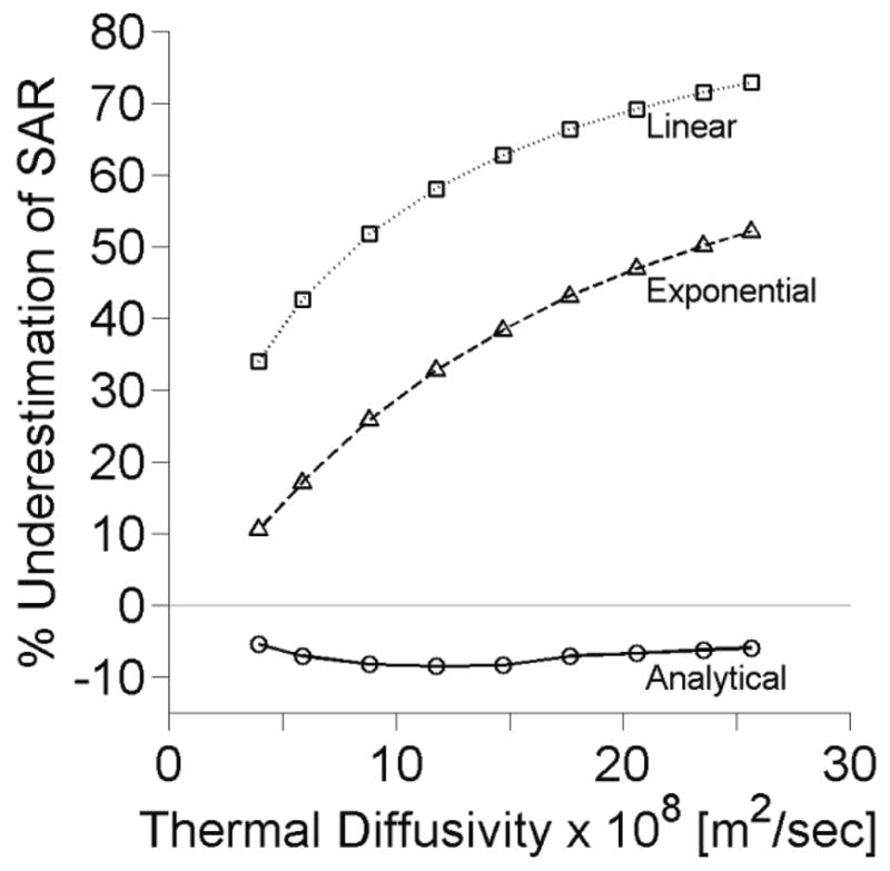
Effects of tissue thermal diffusivity upon SAR estimation at the center of the focal zone with other parameters set at nominal values.

Increasing the acoustic power level from the nominal 5 acoustic watts to 10 and 15 acoustic watts yields results identical to those presented in figures 2 through 5. Hence, variation in acoustic power level has no effect upon the accuracy of SAR regardless of estimation method or parameter values.

3.3 Effects of spatial variation on SAR estimation

Figures 6(a), 6(b), and 6(c) show SAR estimation as a function of lateral position for the small, medium, and large focal zones, respectively. Each lateral profile shown is at the depth of the maximum SAR. These results used the first off-axis analytical fitting approach described in section 2.2.3 with equation (18). The off-axis analytical method reproduces the SAR profile more accurately than the linear and exponential methods for all focal zone sizes. No results are presented for the extended analytical method since it cannot be applied for off-axis locations.

Figure 6.

Lateral SAR estimation using the linear, exponential and off-axis analytical methods for (a) small, (b) medium, and (c) large focal zone sizes at the depth of maximum SAR with other parameters set at nominal values.

In figures 7(a), 7(b), and 7(c), the axial SAR estimates are shown for the small, medium, and large focal zones, respectively. Each axial location lies on the axis of the ultrasound beam (r=0). The analytical method is the most accurate predictor of SAR for all focal zone sizes. The linear and exponential methods underestimate SAR within the focal zone and improve as focal zone size increases. The extended analytical method results (not shown) matched the analytical method to within ±2%.

Figure 7.

Axial SAR estimation using the linear, exponential and on-axis analytical methods for (a) small, (b) medium, and (c) large sized focal zones along the axis of beam propagation with other parameters set at nominal values.

4. Experimental Results

4.1 Experimentally estimated SAR

Lateral SAR patterns estimated from experimental heating of the tissue-mimicking phantom are shown in figure 8 at the depth of maximum temperature elevation. The estimated lateral FWHM of the ultrasound beam is 3.08 mm, 2.58 mm, and 2.03 mm for the linear, exponential, and analytical fitting methods, respectively.

Figure 8.

Lateral profiles for experimentally determined SAR at the depth of maximum heating.

4.2 Experimental and simulated temperature comparisons

The lateral distributions of the experimental temperatures and calculated temperatures (based on experimentally obtained SAR values) are shown in figure 9 for four different times during the heating period at the depth of maximum temperature elevation. The analytical method for estimating SAR matches experimental FWHM of temperatures with less than ±5% error and has a maximum temperature error of approximately 1° C. The linear estimation method provides a lateral FWHM 28–38% wider than experimental results and underestimates the maximum temperature by almost 6° C, while the exponential method overestimates the lateral FWHM by 13–21% and underestimates temperatures by up to 2° C.

Figure 9.

Lateral temperature distributions of experimental temperatures and calculated temperatures from heating patterns acquired using different SAR estimation methods at heating times of (a) 3.1 sec, (b) 8.1 sec, (c) 13.1 sec, and (d) 18.1 sec.

5. Discussion

The analytical method clearly estimates SAR more accurately than the linear and exponential methods. Importantly, it does so very robustly, with less than 10% error- independent of beam size, tissue properties (excluding high perfusions), applied power, and fitting parameters. It has the additional advantage that it can be applied to find SAR estimates at off-axis focal zone positions and can be altered to include perfusion effects at the center of the focal zone. Application of the standard linear SAR estimation method, while valid fo or applications with heating modalities with diffuse SAR patterns, should be avoided for HIFU SAR estimation except where temperature sampling intervals can be made very small. While the exponential SAR estimation method is consistently more accurate than the linear method, it is inferior when compared with the analytical results.

5.1 The standard linear method

The primary advantage of the frequently used linear method is its simplicity- it applies a single-parameter fit to the temperatures. While the assumption of linearity makes the solution simple, it also provides the prime source of error in the method. In HIFU treatments, the focal zone is so small and the spatial temperature gradients so large that conduction effects become apparent almost immediately, limiting the accuracy of the linear method.

Only when the sampling interval and total time for fit are reduced to 0.25 sec, which is difficult to accomplish experimentally, is the linear SAR estimation error less than 10%. This is consistent with Parker’s criterion (4κt_tot/β ≤ 0.1) for use of the linear approximation when estimating acoustic absorption (1985).

5.2 The exponential method

The motivation for testing the exponential method is the desire to introduce a simple model of curvature to the fitting procedure. While this solution is simple, conduction effects are not exponential in nature but vary with time as the spatial second derivative of temperature changes. Because of this, the exponential solution does not match the temperature rise as well as the analytical fit. However, with increasing focal zone size, the spatial temperature gradients are reduced, conduction losses decrease, and SAR estimates using the exponential fit are increasingly more accurate (figures 6 and 7).

Like the linear method, the exponential SAR estimation method has its lowest errors for the minimum total time for fit and in tissues with low thermal diffusivity. The improved accuracy of SAR estimations with short total times for the fit suggests that an exponential curve may be used as a reasonable approximation for the time-temperature curve for short periods of time. It should be noted that, for very short fitting times (<1 sec for the nominal case), the temperature versus time curve does indeed approach linearity and attempting to apply an exponential curvature causes slight overestimation of the initial slope and SAR (figure 2(b)).

5.3 The analytical method: Simulation results

At the center of the focal zone, the analytical method for estimating SAR employs a two-parameter least-squares fit to the temperature versus time data. The method assumes a 1-D radial Gaussian SAR profile, while neglecting perfusion and axial conduction. Results indicate that these approximations are quite accurate for estimating SAR in HIFU if perfusion levels are less than 5 kg/(m³·s). The analytical method yields less than 10% error at the center of the focal zone, regardless of tissue properties or experimental parameters (excluding high perfusions).

It is possible that that neglecting perfusion and axial conduction causes the slight, but consistent overestimation in SAR using the analytical method. Since these two heat loss mechanisms are not accounted for by the analytical solution, the analytical method’s fitting process compensates by increasing the model’s radial conduction, which is determined by the fitting parameter D. For each of the simulations, the estimated parameter D was larger than its true value. From its definition, D=4κ/β, overestimating D implies that either the thermal diffusivity has increased or the Gaussian variance, a measure of the beam width, has decreased. Either of these changes would cause an increase in radial conduction. Overestimation of D with increased SAR at the center of the focal zone generates the temperature gradients necessary to account for perfusion and axial heat losses when only radial conduction is present. Though incorrect physically, this compensation provides SAR results that are significantly more accurate than the linear and exponential methods. Only for very short fitting times (<1 sec) and larger focal zones (lateral FWHM> 2.6 mm) can the exponential and linear methods provide SAR estimates comparable in accuracy to the analytical solution.

The acquisition time (i.e. sampling interval) of MRTI sequences can range from approximately one second to greater than five seconds, depending upon the desired field of view, spatial resolution, and signal-to-noise ratio requirements. Figure 2 shows that the analytical method is essentially independent of the sampling interval t_s. This result suggests that by using the analytical method, HIFU researchers using MRTI may implement longer acquisition times to improve spatial resolution without significantly affecting SAR estimation accuracy.

Many tissues of interest in HIFU thermal therapies have low perfusion levels. Resting muscle and fat, for example, each have perfusion levels less than 0.65 kg/(m³·s). In these tissues, using the simple analytical solution will provide SAR estimates accurate to within 10%. However, other tissues such as the kidney may have perfusion levels up to, and even exceeding, 50 kg/(m³·s) (Duck 1990). In such cases, it is advantageous to use the analytical solution including perfusion developed by Kress. While this solution is only available at the center of the focal zone, SAR errors using this analytical fit remain less than 10% even for very high perfusion rates (figure 4).

Each of the estimation methods requires knowledge of the tissue specific heat. Errors in specific heat values will alter SAR estimation accuracy in a linear fashion. This is motivation for obtaining patient specific property values for HIFU treatment planning.

5.4 The analytical method: Experimental results

Applying the estimation methods to experimental data verified the simulation results that the magnitude and spatial distribution of SAR can be accurately estimated from temperature versus time data with the analytical method.

Using the MRTI temperature field, the beam axis location is easily identified, and therefore every voxel’s radial position r can also be accurately determined with uncertainty in r no greater than the in-plane voxel dimensions. Knowledge of r provides additional information to the off-axis analytical solution so the thermal diffusivity, κ, and ultrasound Gaussian variance, β, can be estimated directly (see section 2.2.3). These estimates are most accurate at the depth of maximum SAR, where the model’s approximations are most valid. From the experimental data, the thermal diffusivity of the ATS phantom was estimated at 1.49×10⁻⁷ m²/sec, 7.2% higher than the value given by the manufacturer. While κ was slightly overestimated, the fit for β appears to be reasonably accurate since lateral distributions of the experimental and calculated temperatures match to ±5% throughout the heating. Given the discussion on parameter D in section 5.3, these results were expected.

There are several advantages to fitting temperature data for several voxels simultaneously in the experimental validation. Computationally, the simultaneous parameter estimation at each of the 64 axial depths reduced the number of fits necessary to estimate SAR for the entire 3-D field from ~400,000 to 64, thus reducing computation time from several hours to approximately one minute. Additionally, using simultaneous parameter estimation significantly reduces the effects of noise that are present when estimates are generated for each voxel independently.

The primary disadvantage of using data from many locations for simultaneous parameter estimation is that the estimated SAR is constrained to a Gaussian distribution at each axial depth. This is a very good approximation near the center of the focal zone but becomes increasingly tenuous at axial depths away from the center. This approximation may also be less valid when estimating SAR in inhomogeneous tissue or when the beam is steered significantly in the lateral direction. Finally, because the assumption of a Gaussian distribution quickly forces the estimated SAR to zero at locations lateral to the focal zone, this method is not effective in quantifying the effects of ultrasound side lobes, grating lobes, and scattering outside the focus.

In addition to improving SAR estimation, the analytical temperature solutions (12), (16), and (20) could be applied in other ways to improve HIFU treatments. For example, the solutions could be used in model predictive filtering techniques (Todd et al 2010) to improve MRI temperature coverage and increase both spatial and temporal resolution. In a real-time controller, forward predicting the temperatures with analytical solutions could be applied for thermal dose optimization. The solutions could also help to eliminate the effects of temperature acquisition artifacts, such as viscous heating (Goss et al 1977).

Assumptions necessary to the experimental validation are that the MR temperatures are accurate, the published and measured thermal properties used in thermal models are accurate, and that the FD thermal model accurately represents the heating process in the treatment volume. Quantifying effects of MR noise, temporal and spatial averaging, uncertainty in power-on time, and partial volume effects is left for future studies. The effects of acoustic non-linearity and tissue inhomogeneity on SAR estimation were also not assessed in this study. However, if these effects do not alter the nearly Gaussian nature of the ultrasound beam, the analytical method should remain accurate.

6. Conclusion

The primary finding of this study is that the 1-D radial Gaussian analytical solution for estimating SAR is a significant improvement over the standard linear method and the simple exponential method. The analytical method estimates SAR with a high degree of accuracy, independent of beam size, tissue properties, power level, and temperature sampling intervals. At low perfusion levels, the simple analytical solution can be used to acquire SAR estimates at all axial and lateral locations. For highly perfused tissues, the extended analytical solution including perfusion provides accurate SAR estimates at the center of the focal zone. When applying the method to experimental data, noise effects in SAR estimation can be significantly reduced by performing a simultaneous parameter estimation to the temperature versus time data for longer times and for several locations at each axial depth. Using this method also provides estimates for the thermal diffusivity and ultrasound Gaussian variance. The improved analytical SAR estimation method should be useful for the comparison of results from different HIFU studies and for the validation of SAR predictive software used in patient treatment planning of HIFU thermal therapies.

Nomenclature

A

Fitting parameter °C/sec

B

Fitting parameter °C

c

Speed of sound m/sec

c_p

Specific heat J/(kg·°C)

C

Fitting parameter °C/sec

D

Fitting parameter sec⁻¹

F

Fitting parameter dimensionless

I_o

Ultrasound intensity W/m²

k

Thermal conductivity W/(m·°C)

Q

Power deposition density W/m³

r

Radial distance from the beam axis m

SAR

Specific absorption rate W/kg

t

Time sec

t_s

Sampling interval sec

t_tot

Total time for fit sec

T

Tissue temperature elevation from reference temperature °C

T_ar

Arterial blood temperature °C

T_PD

Temperature elevation (Pulse decay) °C

T_SH

Temperature elevation (Step-heating) °C

w

Perfusion coefficient kg/(m³·sec)

w_loss

Effective heat loss coefficient kg/(m³·sec)

α

Ultrasound absorption coefficient Np/m

β

Ultrasound Gaussian variance m²

γ

Fitting parameter dimensionless

κ

Thermal diffusivity m²/sec

ρ

Density kg/m³

τ

Fitting parameter sec

References

- Arkin H, Holmes KR, Chen MM, Bottje WG. Thermal pulse decay method for simultaneous measurement of local thermal conductivity and blood perfusion: a theoretical analysis. J Biomech Eng. 1986;108:208–14. doi: 10.1115/1.3138604. [DOI] [PubMed] [Google Scholar]
- Cheng HL, Plewes DB. Tissue thermal conductivity by magnetic resonance thermometry and focused ultrasound heating. J Magn Reson Imaging. 2002;16:598–609. doi: 10.1002/jmri.10199. [DOI] [PubMed] [Google Scholar]
- Cheng KS, Roemer RB. Blood perfusion and thermal conduction effects in Gaussian beam, minimum time single-pulse thermal therapies. Med Phys. 2005;32:311–7. doi: 10.1118/1.1835591. [DOI] [PubMed] [Google Scholar]
- Damianou CA, Sanghvi NT, Fry FJ, Maass-Moreno R. Dependence of ultrasonic attenuation and absorption in dog soft tissues on temperature and thermal dose. J Acoust Soc Am. 1997;102:628–34. doi: 10.1121/1.419737. [DOI] [PubMed] [Google Scholar]
- De Poorter JD, De Wagter C, De Deene Y, Thomsen C, Stahlberg F, Achten E. Noninvasive MRI thermometry with the proton resonance frequency (PRF) method: in vivo results in human muscle. Magn Reson Med. 1995;33:74–81. doi: 10.1002/mrm.1910330111. [DOI] [PubMed] [Google Scholar]
- Diederich CJ, Clegg S, Roemer RB. A spherical source model for the thermal pulse decay method of measuring blood perfusion: a sensitivity analysis. J Biomech Eng. 1989;111:55–61. doi: 10.1115/1.3168340. [DOI] [PubMed] [Google Scholar]
- Dragonu I, de Oliveira PL, Laurent C, Mougenot C, Grenier N, Moonen CTW, Quesson B. Non-invasive determination of tissue thermal parameters from high intensity focused ultrasound treatment monitored by volumetric MRI thermometry. NMR Biomed. 2009;22:843–51. doi: 10.1002/nbm.1397. [DOI] [PubMed] [Google Scholar]
- Duck FA. Physical Properties of Tissue: A Comprehensive Reference Book. New York: Academic; 1990. [Google Scholar]
- Gladman AS, Davidson SRH, Easty AC, Joy ML, Sherar MD. Infrared thermographic SAR measurements of interstitial hyperthermia applicators: errors due to thermal conduction and convection. Int J Hyperthermia. 2004;20:539–55. doi: 10.1080/02656730410001668366. [DOI] [PubMed] [Google Scholar]
- Goss SA, Cobb JW, Frizzell LA. Effect of beam width and thermocouple size on the measurement of ultrasonic absorption using the thermoelectric technique. IEEE Ultrasonics Symp Proc. 1977:206–11. [Google Scholar]
- Guy AW, Lehmann JF, Stonebridge JB. Therapeutic applications of electromagnetic power. Proc of the IEEE. 1974;62:55–75. [Google Scholar]
- International Commission on Radiation Units and Measurements. ICRU Report 61: Tissue Substitutes, Phantoms and Computational Modelling in Medical Ultrasound. ICRU Publications; Bethesda, Maryland: 1998. [Google Scholar]
- Ishihara Y, Calderon A, Watanabe H, Okamoto K, Suzuki Y, Kuroda K, Suzuki Y. A precise and fast temperature mapping using water proton chemical shift. Magn Reson Med. 1995;33:814–23. doi: 10.1002/mrm.1910340606. [DOI] [PubMed] [Google Scholar]
- Kharalkar NM, Hayes LJ, Valvano JW. Power-pulse integrated-decay technique for the measurement of thermal conductivity. Meas Sci Technol. 2008;19:075104. [Google Scholar]
- Kress R, Roemer R. A comparative analysis of thermal blood perfusion measurement techniques. J Biomech Eng. 1987;109:218–25. doi: 10.1115/1.3138672. [DOI] [PubMed] [Google Scholar]
- Mahoney K, Fjield T, McDannold N, Clement G, Hynynen K. Comparison of modelled and observed in vivo temperature elevations induced by focused ultrasound: implications for treatment planning. Phys Med Biol. 2001;46:1785–98. doi: 10.1088/0031-9155/46/7/304. [DOI] [PubMed] [Google Scholar]
- Nyborg WL. Solutions of the bio-heat transfer equation. Phys Med Biol. 1988;33:785–92. doi: 10.1088/0031-9155/33/7/002. [DOI] [PubMed] [Google Scholar]
- Parker KJ. The thermal pulse decay technique for measuring ultrasonic absorption coefficients. J Acoust Soc Am. 1983;74:1356–61. [Google Scholar]
- Parker KJ. Effects of heat conduction and sample size on ultrasonic absorption measurements. J Acoust Soc Am. 1985;77:719–25. doi: 10.1121/1.392340. [DOI] [PubMed] [Google Scholar]
- Payne A, Vyas U, Todd N, de Bever J, Christensen DA, Parker DL. The effect of electronically steering a phased array ultrasound transducer on near-field tissue heating. Med Phys. 2011;38:4971–81. doi: 10.1118/1.3618729. [DOI] [PMC free article] [PubMed] [Google Scholar]
- Pennes HH. Analysis of tissue and arterial blood temperatures in the resting human forearm. J Appl Physiol. 1948;1:93–122. doi: 10.1152/jappl.1948.1.2.93. [DOI] [PubMed] [Google Scholar]
- Roemer RB, Fletcher AM, Cetas TC. Obtaining local SAR and blood perfusion data from temperature measurements: steady state and transient techniques compared. Int J Radiation Oncology Biol Phys. 1985;11:1539–50. doi: 10.1016/0360-3016(85)90343-8. [DOI] [PubMed] [Google Scholar]
- Samaras T, van Rhoon GC, Sahalos JN. Theoretical investigation of measurement procedures for the quality assurance of superficial hyperthermia applicators. Int J Hyperthermia. 2002;18:416–25. doi: 10.1080/02656730210132039. [DOI] [PubMed] [Google Scholar]
- Sherar MD, Gladman AS, Davidson SRH, Trachtenberg J, Gertner MR. Helical antenna arrays for interstitial microwave thermal therapy for prostate cancer: tissue phantom testing and simulations for treatment. Phys Med Biol. 2001;46:1905–18. doi: 10.1088/0031-9155/46/7/312. [DOI] [PubMed] [Google Scholar]
- Todd N, Payne A, Parker DL. Model predictive filtering for improved temporal resolution in MRI temperature imaging. Magn Reson Med. 2010;63:1269–79. doi: 10.1002/mrm.22321. [DOI] [PMC free article] [PubMed] [Google Scholar]
- Todd N, Vyas U, de Bever J, Payne A, Parker DL. The effects of spatial sampling choices on MR temperature measurements. Magn Reson Med. 2011;65:515–21. doi: 10.1002/mrm.22636. [DOI] [PMC free article] [PubMed] [Google Scholar]
- Valvano JW, Allen JT, Bowman HF. The simultaneous measurement of thermal conductivity, thermal diffusivity, and perfusion in small volumes of tissue. J Biomech Eng. 1984;106:192–7. doi: 10.1115/1.3138482. [DOI] [PubMed] [Google Scholar]
- Vyas U, Christensen DA. Ultrasound beam simulations in inhomogeneous tissue geometries using the hybrid angular spectrum method. IEEE Trans Ultrason, Ferroelectr, Freq Control. 2012;59:1093–100. doi: 10.1109/tuffc.2012.2300. [DOI] [PubMed] [Google Scholar]
- Vyas U, Todd N, Payne A, Parker D, Christensen DA. Non-invasive ultrasound tissue property measurement using MRI temperature maps of low-powered heating. Annual Mtg. of Soc. Thermal Med; Clearwater, FL. 2010. Apr 23–26, [Google Scholar]
- Zderic V, Keshavarzi A, Andrew MA, Vaezy S, Martin RW. Attenuation of porcine tissues in vivo after high-intensity ultrasound treatment. Ultrasound Med Biol. 2004;30:61–6. doi: 10.1016/j.ultrasmedbio.2003.09.003. [DOI] [PubMed] [Google Scholar]