Robustness of Cortical Topography across Fields, Laminae, Anesthetic States, and Neurophysiological Signal Types

Abstract

Topographically organized maps of the sensory receptor epithelia are regarded as cornerstones of cortical organization as well as valuable readouts of diverse biological processes ranging from evolution to neural plasticity. However, maps are most often derived from multiunit activity recorded in the thalamic input layers of anesthetized animals using near-threshold stimuli. Less distinct topography has been described by studies that deviated from the formula above, which brings into question the generality of the principle. Here, we explicitly compared the strength of tonotopic organization at various depths within core and belt regions of the auditory cortex using electrophysiological measurements ranging from single units to delta-band local field potentials (LFP) in the awake and anesthetized mouse. Unit recordings in the middle cortical layers revealed a precise tonotopic organization in core, but not belt, regions of auditory cortex that was similarly robust in awake and anesthetized conditions. In core fields, tonotopy was degraded outside the middle layers or when LFP signals were substituted for unit activity, due to an increasing proportion of recording sites with irregular tuning for pure tones. However, restricting our analysis to clearly defined receptive fields revealed an equivalent tonotopic organization in all layers of the cortical column and for LFP activity ranging from gamma to theta bands. Thus, core fields represent a transition between topographically organized simple receptive field arrangements that extend throughout all layers of the cortical column and the emergence of nontonotopic representations outside the input layers that are further elaborated in the belt fields.

Introduction

The empirical age of cortical cartography began with the discovery that the neural processes underlying vision, touch, and audition could be ascribed to discrete areas of the cerebral cortex, each containing topographically organized maps of the corresponding sensory receptor epithelia (Larionow, 1899; Woolsey and Walzl, 1942). As the tools advanced from lesions and surface potential recordings to neuroanatomical tracers and dense microelectrode mapping, it became possible to delineate multiple fields within the cortical areas representing a single modality, as well as their distinct patterns of interconnections and functional specializations (Merzenich et al., 1975; Read et al., 2001). The latest wave of optical physiological tools offers the promise of penetrating still further into the functional fabric of the cortex by providing spatial resolution at the cellular level and the ability to record and manipulate neural activity on a millisecond timescale (Garaschuk et al., 2006; Fenno et al., 2011).

In the auditory cortex, the smooth and precisely organized tonotopic gradients described by traditional microelectrode mapping studies are incompatible with the heterogeneous frequency organization described by recent two-photon Ca²⁺ imaging studies (Bandyopadhyay et al., 2010; Rothschild et al., 2010). The concept of precise tonotopy, which is regarded as a hallmark characteristic of auditory core fields, has arisen almost exclusively from studies using a single experimental approach: measuring threshold frequency tuning from multiunit (MU) recordings in the middle cortical layers of anesthetized animals. The disparate findings from Ca²⁺ imaging raise the possibility that precise tonotopy may be an epiphenomenon of this heavily used methodology rather than the singular valid description of the underlying biology. Indeed, the minority of studies that have described poor frequency selectivity, heterogeneous local frequency tuning, or weakly organized maps all deviate from the methodological formula above by characterizing preferred frequency with suprathreshold sound levels, recording outside of the thalamic input layers, recording in unanesthetized subjects, and/or recording neural activity other than MU spiking such as evoked potentials, local field potentials (LFPs), neuronal Ca²⁺ transients, magneto-encephalographic signals, or blood oxygenation level-dependent functional magnetic resonance imaging (fMRI) signals (Evans et al., 1965; Goldstein et al., 1970; Woods et al., 1995; Bilecen et al., 1998; Schönwiesner et al., 2002; Kaur et al., 2004; Kayser et al., 2007; Chen et al., 2011; Gaucher et al., 2011).

Disambiguating the contribution of each variable to tonotopic map precision is challenging because the studies listed above have been conducted in a variety of species and, within a given study, only compare tuning quality across one of these variables, if at all. Therein lies the motivation for the present study: first, we elected to use the mouse auditory cortex as a test bed, as it has alternately been described as having a heterogeneous frequency representation based on Ca²⁺ imaging in the superficial layers or a precise tonotopic organization based on MU mapping in the middle layers (Stiebler et al., 1997; Hackett et al., 2011). Then, we explicitly compared the contributions of five variables that are thought to modulate the strength of topographic mapping: (1) the cortical field of the recording site (auditory core vs belt fields); (2) the sound level used to estimate frequency tuning; (3) the cortical layer from which recordings are made; (4) the kind of activity used to estimate map organization [MU spiking, single unit (SU) spiking, or LFP amplitude]; and (5) the state of the animal (anesthetized vs awake).

Materials and Methods

Surgical procedures

Anesthetized recordings.

All procedures were approved by the Animal Care and Use Committee at Massachusetts Eye and Ear Infirmary and followed the guidelines established by the National Institutes of Health for the care and use of laboratory animals. Female CBA/CaJ mice aged 8–10 weeks were brought to a surgical plane of anesthesia either with ketamine/xylazine (induction with 120 mg/kg ketamine and 12 mg/kg xylazine, with 60–80 mg/kg ketamine supplements as necessary) or pentobarbital sodium/chlorprothixene (induction with 50 mg/kg pentobarbital and 0.2 mg chlorprothixene, followed by 10–15 mg/kg pentobarbital supplements, as necessary). Using a scalpel, a 4 × 3 mm (rostrocaudal × mediolateral) craniotomy was made in the right auditory cortex, approximately centered on a point 2.8 mm posterior and 4.4 mm lateral to bregma, and the dura mater was left intact. The brain surface was covered with high-viscosity silicon oil and photographed. During the course of recording, the core body temperature of the animal was maintained at 36.5°C with a homeothermic blanket system (Fine Science Tools). The animal was administered 0.5 ml lactated Ringer's solution every 6 h to prevent dehydration.

Acute awake recordings.

A titanium head plate, 37.3 × 5.2 × 0.9 mm (L × W × H) weighing 0.5 g, was first affixed to the animal's skull under isoflurane anesthesia (5% induction, 2.5% maintenance) several days before head-fixed recordings began. The dorsal surface of the skull was exposed, a thin layer of tissue adhesive (VetBond; 3M) applied, and the headplate affixed to the dorsal aspect of the skull overlying bregma with acrylic bonding material (C&B Metabond; Parkell). A silver ground wire (0.005 inch diameter; A-M Systems) was inserted through a small hole made in the skull and fixed into place using tissue adhesive and acrylic following contact with the dura. The wound margin was numbed (burprivaine 0.05%) and sealed with tissue adhesive. Subcutaneous injections of buprenorphine (0.05 mg/kg) and saline (0.5 ml) were given to reduce pain and dehydration, respectively.

On the day of recording, the animal was anesthetized with isoflurane so that the experimenter could inspect the ear canal, attach a pinna insert for sound delivery, and perform a craniotomy. During the ear canal inspection, a small slit was made at the base of the left pinna to better visualize the tympanic membrane. A funnel-shaped plastic insert (1.2 cm long, 4.3 mm and 1.4 mm diameters for the ends facing the speaker assembly and the tympanic membrane, respectively) was affixed to the external auditory meatus with cyanoacrylate gel. A 2.5 × 1.5 mm (caudorostral × mediolateral) craniotomy was made medial to the squamosal suture and 2–3 mm rostral to the lambdoid suture with the dura mater left intact. The animal was typically ambulatory and showing normal behaviors such as whisking and grooming within 3–5 min following cessation of isoflurane. Recordings were delayed for an additional 50 min to ensure that the animal was fully awake during the electrophysiology experiment. The animal was restrained during recording by immobilizing the headplate and positioning the body in a cylindrical plastic tube. Animals were adapted to the restraint apparatus at least 24 h before the recording experiment.

Chronic awake recordings.

In four mice the auditory cortex was implanted with an array of 16 polyimide-coated tungsten microwires (2 rows of 8 electrodes oriented along a caudorostral axis, 50 μm diameter cut at a 30 degree angle, 250 μm spacing between wires; Tucker-Davis Technologies). Details relating to subjects, anesthesia, surgery, and postsurgical analgesia procedures were identical to the acute awake preparation described above. The implant was fixed onto the dorsal surface of the skull overlying the right auditory cortex with dental bonding material. A bone screw was fixed into the skull overlying the left occipital cortex for use as a ground. Recordings were obtained 1–2 weeks after the implant surgery.

Data collection

Acute extracellular recordings.

Simultaneous recordings were made from the middle layers of the auditory cortex (420–430 μm from pial surface) with 2–4 epoxylite-coated tungsten microelectrodes (1–2 MΩ at 1 kHz; FHC). To enable more direct comparisons to unbiased approaches such as cell-attached recordings (Hromádka et al., 2008) and two-photon Ca²⁺ imaging (Bandyopadhyay et al., 2010; Rothschild et al., 2010), the final positions of the recording electrodes were not adjusted to find units most responsive to an auditory search stimulus or to isolate the most prominent SU waveforms. For columnar comparisons, the primary auditory cortex (A1) and the anterior auditory field (AAF) were first identified through a coarse mapping of middle layer responses. Next, a 16-channel silicon probe (177 μm² contact area, 50 μm contact separation; NeuroNexus Technologies) was inserted orthogonal to the brain surface in A1 or AAF (as confirmed through postmortem electrode track reconstructions in a subset of cases) until the topmost recording channel was level with the pial surface. The location of each recording site was marked on a high-resolution photograph of the brain surface.

Chronic extracellular recordings.

For direct comparison between awake and anesthetized recordings in the same animals, the four mice with implanted multi-electrode arrays were first tested in the awake condition. The animal was allowed to move ad libitum within an 11 × 11 cm acoustically transparent enclosure during recording. Immediately after the awake recording session, the animal was anesthetized with an intraperitoneal injection of ketamine (100 mg/kg) and xylazine (10 mg/kg) with all other conditions held constant. All awake and anesthetized recording experiments (both acute and chronic) were performed inside a double-walled sound-attenuating test chamber (ETS-Lindgren).

Acoustic stimuli.

Stimuli were generated with a 24-bit digital-to-analog converter (National Instruments model PXI-4461). In acute recording sessions, stimuli were presented via acoustic assemblies consisting of two miniature dynamic earphones (CUI CDMG15008–03A) and an electret condenser microphone (Knowles FG-23339-PO7) coupled to a probe tube. Stimuli were calibrated at the tympanic membrane in each mouse before recording. Normal function of the auditory periphery and accurate placement of the probe tube were confirmed by monitoring the threshold and amplitude of cochlear distortion product oto-acoustic emissions at frequency 2f1-f2 (ratio of the primary and secondary tone frequencies [f2/f1] = 1.2, sound level of tone at f1 was 10 dB greater than the tone at f2, and f2 = 8, 11.3, 16, 22.6, 32 kHz). In chronic recordings, stimuli were presented via a free-field electrostatic speaker (Tucker-Davis Technologies) placed 17 cm from the center of the enclosure. Free-field stimuli were calibrated before recording with a wide-band ultrasonic acoustic sensor (Knowles Acoustics, model SPM0204UD5).

Frequency response areas (FRAs) were measured with pseudorandomly presented tone pips (50 ms duration, 4 ms raised cosine onset/offset ramps, 0.5–1 s intertrial interval) of variable frequency (4–64 kHz in 0.1 octave increments) and level (0–60 dB SPL in 5 dB increments). A total of 533 unique frequency-level combinations were presented once or twice for a given recording site.

Data processing.

Raw signals were digitized at 32-bit, 24.4 kHz (RZ5 BioAmp Processor; Tucker-Davis Technologies) and stored in binary format. Subsequent analyses were performed in MATLAB 2011a (MathWorks). The signals were notch filtered at 60 Hz and then bandpass filtered at 300–5000 Hz with a fifth-order acausal Butterworth filter. MU spikes were detected as threshold-crossing events using an adaptive threshold (4.5 SDs from the mean of a 10 s running average for standard MU recordings, except where otherwise noted). Well-isolated SUs were identified in a subset of recording sites according to their interspike interval distributions (modal interval occurring later than 5 ms, no intervals <2 ms) and waveform consistency (average deviation of the waveforms from the mean waveform of the cluster <15 μV). For LFPs, the raw signals were down-sampled to 1 kHz and bandpass filtered at each frequency band using fifth-order causal Butterworth filters to avoid backward temporal spreading of the filtering artifacts. The delays introduced by the filters were corrected subsequently by shifting the filtered signals in the time domain to maximize their alignment with the original signals.

Data analysis

FRA analysis.

A poststimulus time histogram (PSTH) was calculated for each recording site with 1 ms bin size. To identify sound-driven recording sites, the spike counts before and after tone onset were compared between two 100 ms windows in the PSTH, one set to begin 150 ms before tone onset and the other set to capture the 100 contiguous poststimulus bins with the greatest number of events. Sites with significant increase in spike counts after tone onset (p < 0.01, unpaired t test) were classified as sound driven. Next, the PSTH for each sound-driven unit was windowed to capture stimulus-related spikes. The start of the window (response onset) was set to be the point when the firing rate began to consistently exceed the spontaneous rate by at least 4 SD. The offset of the spike collection window was set to either 20 ms after the modal bin or the first bin after the response decreased to <5 SD above the spontaneous rate. Only spike events occurring within this window were used in FRA determination. For LFP data, the analytical amplitudes of the traces, calculated from the Hilbert transform, were used to represent the response amplitudes. The LFP signals were then analyzed in a fashion similar to the spike data, except that the length of the analysis window was adjusted to fit the wavelength of the signal in each frequency band.

FRA boundaries were quantified using an automated objective method to isolate the contiguous tone-evoked response areas. The FRA was first smoothed by a 3 × 3 point median filter, then the spike counts were summed across sound frequencies or sound levels to create spike-frequency or spike-level functions, each of which were subsequently smoothed again with a 5-point median filter. The spike-frequency function was inverted (to create a V shape) and the tip set at the minimum threshold, defined as the inflection point on the spike-level function. The resultant FRA outline exhibited a high degree of concordance with subjective estimates of the tone-driven and tone-unrelated regions (see Fig. 1B). With the FRA boundary shape established, all subsequent analysis on the tone-driven versus tone-unrelated portions of the FRA was performed on the “raw” tone-evoked spike counts.

Figure 1.

Organization of core and belt auditory fields in the mouse cortex. A, An exemplary tessellated BF map delineated from 300 MU recording sites in the middle layers of mouse auditory cortex. Polygon size is proportional to the spacing of adjacent penetrations. Polygon color reflects BF. Black dots represent unresponsive sites. B, Example FRAs measured from the recording sites marked in A. Lighter colors represent higher spike counts. Tone-driven FRA region is enclosed by white outline. Vertical gray lines denote BF. Response quality for each site is represented by d′ value derived from comparison of tone-driven and tone-unrelated FRA regions. C, Schematized organization of the mouse auditory cortex, identifying the relative position of five auditory fields. Core fields are shaded gray. Arrows in core fields represent the low (L) to high (H) tonotopic axes. Blue-shaded region denotes core A1 and AAF described in our recent study (Hackett et al., 2011). Yellow-shaded region denotes the area previously described as the ultrasonic field (Stiebler et al., 1997). D, Relative position of auditory fields in four cases where several, but not all, fields were mapped. Ellipses represent the location of A1. L, lateral; R, rostral; A1, primary auditory cortex; AAF, anterior auditory field; DP, dorsal posterior auditory field; A2, secondary auditory cortex; IAF, insular auditory field. Scale bar, 0.5 mm.

The tone-driven portion of the FRA was used to determine the best frequency (BF), the frequency associated with the highest spike count summed across all sound levels, and the FRA bandwidth measured 10 dB above the minimum response threshold. To characterize the responsiveness to pure tones, 30 frequency-level combinations were sampled at random from the tone-driven and tone-unrelated portions of the raw FRA, and the mean spike counts of the two subsampled groups were calculated. This process was repeated 1000 times, yielding estimates of the distributions of the mean spike counts for both driven and undriven responses. The d′ of the unit was defined as the difference between the means of these two distributions divided by their arithmetic average SD, reflecting the difference between the spike counts in the driven and undriven FRA regions relative to inherent variability (a measure of the responsiveness of the unit). If the tone-driven portion of the FRA contained <50 tone-level combinations, additional random samples from the tone-unrelated portion were added to reach 50 samples (resulting in a conservative estimate of the unit responsiveness).

Identification of multiple auditory fields.

Cortical fields were manually identified for each animal. Specifically, two regions comprised of units with low-frequency BFs (≤8 kHz) at the caudal and rostral extremes of the map were identified as the caudal end of A1 and the rostral end of AAF, respectively (see Fig. 1A). An area tuned to high frequencies (≥40 kHz) on the medial end of the map was identified as the shared boundary separating A1 and AAF. Two tonotopic axes were defined centered on the low-to-high tonotopic gradient running through the center of A1 and AAF. Boundaries of the surrounding belt fields were then drawn by identifying shifts in response properties and receptive fields along isofrequency contours oriented orthogonal to the tonotopic axes. In experiments where only the caudorostral extent of A1 and AAF was explored, the BFs of the recording sites were plotted as a function of their caudorostral coordinates, and the inflection point of the curve was used as the boundary between A1 and AAF.

Quantification of tonotopy.

For each pair of recording sites, i and j, located at cortical positions p_i and p_j, respectively, a BF gradient vector was defined as the BF at site i minus the BF at site j, normalized by the Euclidean distance between p_i and p_j, all multiplied by a unit vector in the direction from p_i to p_j as seen in the following:

The resulting gradient, g_ij, points from the site with the lower BF to the site with the higher BF, and has a length proportional to the size of the change in BF normalized by the physical separation of the sites.

For each recording site i, a “tonotopic vector” was defined as the vector average of all the gradients between it and all the other recording sites in the same field as seen in the following:

where Field(i) is the collection of recording sites that belong to the same cortical field as site i, and N_Field(i) is the number of sites in this field.

The tonotopic deviation of field X was defined as the absolute value of the average angular deviation of the tonotopic vectors in the field from the mean tonotopic vector of the field:

where N_X is the number of sites in field X.

Results from the tonotopic vector analysis were plotted on a radian scale and compared using nonparametric statistics, as the values were not normally distributed.

Simulating auditory cortex under two-photon Ca²⁺ imaging.

Simulated two-photon Ca²⁺ imaging maps were compared with unit recordings obtained from the middle layers of auditory cortex. First, a mesh grid with 1 × 1 μm grid size was generated over the MU map. Next, a randomly selected 1% of grid locations were populated with neurons, a ratio that yields a tone-responsive neuron density comparable to what has been published in previous Ca²⁺ imaging studies. Finally, the BFs of the cells were set to be the BF of its closest recording site based on our MU recording recordings, plus or minus a uniformly distributed random jitter covering a 1.5 octave range. This range was based upon data reported in the Ca²⁺ imaging studies (Bandyopadhyay et al., 2010, their Fig. 4; Rothschild et al., 2010, their Fig. 5).

Figure 4.

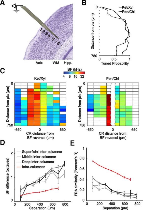
Organization of tonal receptive fields within and between cortical columns in core fields of auditory cortex. A, Schematic of columnar recordings approach. Numbers denote approximate location of cortical layers 1–6. B, Tuned FRA probability as a function of recording depth and anesthetic type. C, Representative columnar maps at 16 depths through central A1 and AAF regions (Fig. 1C, blue-shaded region) under ketamine/xylazine (left, 1 animal) and pentobarbital/chlorprothixene (right, 2 animals) anesthesia. Blank boxes indicate unresponsive or not well tuned sites. D–E, Mean ± SEM absolute value of BF difference (D) or FRA similarity (E) between pairs of well tuned (d′ > 3) recording sites as a function of their distance. Intercolumnar comparisons made at a fixed depth across penetrations were subsequently grouped according to depth (superficial, 0.05–0.25 mm; middle, 0.3–0.5 mm; and deep, 0.55–0.75 mm). Values were computed separately for A1 and AAF then averaged. Actx, auditory cortex; WM, white matter; Hipp., hippocampus; Ket/Xyl, ketamine/xylazine; Pen/Chl, pentobarbital/chlorprothixene. Scale bar, 0.25 mm.

Figure 5.

Impact of irregularly tuned recording sites on tonotopic organization across cortical layers. A–C, Example FRAs and associated PSTHs from each depth and tuning category. Vertical gray lines denote BF. Frequency range, 4–64 kHz; level range, 0–60 dB SPL. D–F, Distributions of d′ values from each depth category. Vertical line denotes the cutoff point used for grouping tuned versus irregularly tuned recording sites. G–I, Scatter plots depict change in BF across the caudorostral extent of A1 based on tuned (filled circles) or irregularly tuned (open circles) recording sites. Solid and dashed straight lines are linear regression lines of tuned and irregularly tuned units, respectively.

Results

Identification and characterization of core and belt fields of the mouse auditory cortex

To delineate the organization of multiple fields within the mouse auditory cortex, MU responses were densely sampled (∼100 μm between neighboring recording sites) in the middle cortical layers under ketamine/xylazine anesthesia. Figure 1A depicts a BF map constructed from 300 recording sites in the right auditory cortex of one mouse. The precise mirror-reversal low-high-low BF gradient that has been used to identify A1 and AAF in at least 20 mammalian species (Kaas, 2011) is immediately evident; FRAs sampled across this gradient (Fig. 1B, recording sites a–f) demonstrate the well structured tonal receptive fields that typify core fields of the auditory cortex. Tone-driven responses were also found lateral and dorsal to the core fields, where tonotopic organization was less distinct and the receptive field quality (as indexed by d′) was lower (Fig. 1B, recording sites g–i).

The “macroscopic” organization of the mouse auditory cortex described here is in close agreement with the seminal report on mouse auditory cortex organization (Stiebler et al., 1997). Borrowing from the terminology used in that study, the zone of mid- and high-frequency tuning dorsal to A1 is the dorsal posterior field (DP) and the field comprised of heterogeneous tuning lateral to A1 is defined as A2 (Fig. 1C). We also observed a small area with mixed BFs rostral to AAF that we denote as the insular auditory field (IAF), in accordance with a recent voltage-sensitive dye-imaging study in the mouse (Sawatari et al., 2011). The only point of departure from the Stiebler (1997) study taxonomy concerned the contiguous zone of highest BFs they described as the ultrasonic field (Fig. 1C, yellow-shaded region). With the higher sampling density used in our study, it was evident that this region is not a separate field, but rather corresponds to the high-frequency extremes of A1 and AAF, an area that was not included in our recent description of the core auditory thalamocortical circuit in the mouse (Fig. 1C, blue-shaded region; Hackett et al., 2011).

The relative position and tonotopic organization of the core and belt fields is also evident in the multifield maps delineated from the right auditory cortices of four additional mice (Fig. 1D). Although the five maps shown in Figure 1 share a common overall framework for the relative layout of various fields and tonotopic gradients within fields, the precise location of borders between fields as well as the detailed point-to-point mapping of BF to a given location differs substantially between individual mice. The individual variation noted here is consistent with the seminal high-density mapping studies of A1 in cats and primates (Merzenich and Brugge, 1973; Merzenich et al., 1973, 1975) and underscores the deleterious effect of creating aggregate maps averaged across multiple animals when delineating precise topography.

Variation in tonotopic mapping strength across the auditory core and belt fields

To determine the degree of tonotopic organization in each field, we calculated the length and angle of vectors derived from local BF gradients (Fig. 2A). In fields with strong tonotopic organization, the distribution of local tonotopic vectors (Fig. 2B, red lines) was tightly clustered around the gradient mean (Fig. 2B, black line), yielding small angular deviations. In addition to BF, many other response properties exhibit spatially ordered representations (Recanzone et al., 1999; Polley et al., 2007; Higgins et al., 2010; Razak, 2011). Although we did not observe any obvious topographic organization of FRA bandwidth (Fig. 2C) or quality (Fig. 2D), we did observe a contiguous area in the caudolateral corner of the auditory cortex that exhibited tone-evoked onset latencies that were longer than all other regions (Fig. 2E), which matched previous reports in the rat (Polley et al., 2007) and cat (Carrasco and Lomber, 2011).

Figure 2.

Spatially organized feature representations in mouse auditory cortex. A, Tonotopic vector map of BFs. B, Distribution of individual vectors shown in A grouped according to field. Black lines indicate the average vectors. C–E, Spatial organization of bandwidth, FRA tuning, and onset latency. F–H, Mean ± SEM bandwidth, FRA d′, and onset latency of each field across animals. I, Median ± interquartile range of tonotopic vector deviation for each field. Lower values indicate more uniform tonotopic gradients. Asterisks denote statistically significant differences relative to A1 (***p < 2.5 × 10⁻⁴, which is the significance level at p < 0.001 after a Bonferroni correction for 4 comparisons; unpaired t test in F–H, Wilcoxon rank sum test in I). Scale bar, 0.5 mm.

Mean values for each of these response properties in A1 (N = 8 mice, 293 recording sites) were compared with AAF (N = 8, 259), DP (N = 6, 110), A2 (N = 8, 120), and IAF (N = 6, 57). Frequency tuning was broader in AAF than in A1 (p = 1.5 × 10⁻⁵, unpaired t test), but comparable to A1 in other fields (Fig. 2F). The FRA quality index (d′) was higher in AAF (p = 1.3 × 10⁻⁵) and lower in IAF (p = 1.6 × 10⁻⁴) than in A1, and was more variable, although not significantly lower or higher, in DP and A2 (Fig. 2G). Compared with A1, tone-evoked spike latencies were shorter in AAF (p = 6.8 × 10⁻¹³), comparable in DP and IAF, and significantly longer in A2 (p = 2.0 × 10⁻¹⁴; Fig. 2H). Returning to the original question of tonotopy, we found that tonotopic deviations in DP, A2, and IAF were significantly greater than A1 (p < 3.3 × 10⁻¹² for all fields, Wilcoxon rank sum test; Fig. 2I). In other words, core fields had a more robust tonotopic organization than belt fields.

Variation in tonotopic mapping strength with threshold versus suprathreshold sound levels

Traditional descriptions of tonotopy define the preferred frequency as the frequency to which the neuron is responsive at its minimum response threshold (i.e., characteristic frequency [CF]) or to which it is most responsive, summing across multiple sound intensities (i.e., BF). In noninvasive imaging studies, maps are often constructed by presenting sounds at a single moderately high intensity (generally 60–80 dB sound pressure level [SPL]). To understand how using threshold versus suprathreshold stimulus amplitudes related to the strength of tonotopy, we compared maps in each field using the BF across sound levels ranging from 0 to 60 dB SPL, CF, and the BF at 60 dB SPL only. Compared with the clear organization seen with BF across all sound levels (Fig. 2A), map organization was well preserved using CF (Fig. 3A), but was significantly degraded when BF was calculated using tones only at 60 dB SPL (Fig. 3B) in A1, AAF, and A2 (p < 0.02 for all tests, significant after correction for multiple comparisons, Wilcoxon rank sum test; Fig. 3C).

Figure 3.

Effect of suprathreshold versus threshold sound levels on tonotopy. A–B, Vector map calculated from CF (A) and BF at 60 dB SPL (B). C, Median ± interquartile range of tonotopic deviation based on BF, CF, BF60, and randomized maps. Asterisks and plus signs indicate statistically significant difference from BF and random conditions, respectively (*/⁺p < 1.7 × 10⁻², **/⁺⁺p < 3.3 × 10⁻³, ***/⁺⁺⁺p < 3.3 × 10⁻⁴, which are the significance levels at p < 0.05, p < 0.01, and p < 0.001, respectively, following a Bonferroni correction for 3 comparisons; Wilcoxon rank sum test). Scale bar, 0.5 mm.

To test if the use of a single, suprathreshold sound level simply reduced tonotopy or actually eliminated it altogether, we calculated the tonotopic mapping strength that resulted from a randomized arrangement of the recording sites in each map. In A1, AAF, and DP, we found that the tonotopy obtained with BF at 60 dB SPL only was still significantly better than chance, albeit significantly worse than BF calculated from all sound levels (p < 0.001 for each comparison). Therefore, characterizing tuning either at threshold or across a number of levels at and above threshold improved the overall precision of tonotopic organization, but was not strictly necessary to find evidence of tonotopicity.

Variation in tonotopic mapping strength between cortical layers

Topographic maps in the cortex are nearly always derived from unit recordings in the middle layers, where thalamocortical synapses are most abundant. Due to physical limitations of optics and the light-scattering properties of brain tissue, the physiological mapping signal acquired with many noninvasive imaging techniques (e.g., Ca²⁺ imaging, intrinsic signal imaging, voltage-sensitive dye imaging, riboflavin imaging) originates in superficial layers of the cortex, where thalamocortical synapses are more sparse and intracortical synapses predominate (Hackett, 2011). We investigated the contribution of cortical recording depth on the characteristics and organization of tonal receptive fields by simultaneously recording MU activities within a cortical column using a multichannel probe oriented orthogonally to the surface of the cortex. As depicted in Figure 4A, this approach enabled us to simultaneously record from the pial surface to a depth of 0.75 mm from the surface, which corresponds to the layer V/VI transition in the mouse (Anderson et al., 2009; Llano and Sherman, 2009).

The probability of recording a tuned MU FRA under ketamine/xylazine anesthesia was greatest in the middle cortical layers (0.3–0.5 mm), tapered off slightly in the deep cortical layers (0.55–0.75 mm), and was reduced even further in the superficial layers (0.05–0.25 mm; Fig. 4B). The loss of tonal receptive fields outside of the middle cortical layers was even more pronounced under pentobarbital/chlorprothixene, where the tuned FRA probability dropped to 50% in the deep layers and was <50% throughout many of the superficial layers. In the event that tuned FRAs were observed across the full length of the recording probe (i.e., at all depths), they exhibited a columnar BF organization. Tonotopic shifts in BF were noted in all layers as the recording probe traversed the caudal-to-rostral frequency gradient spanning A1 and AAF (Fig. 4C).

We directly compared the precision of tonotopic versus columnar organization from well tuned recording sites (d′ > 3) in the core fields. Changes in tonal receptive fields across both the depth axis and the tonotopic axis of A1 and AAF were quantified in two ways: first, by calculating the absolute value of the BF difference at various depths between columns (intercolumnar) and comparing this to the BF change across depths within a single column (intracolumnar; Fig. 4D) and second, by comparing similarity in the overall shape and position of receptive fields between a pair of recording sites (Pearson's R correlation product for spike count at each frequency-level combination for a pair of FRAs) as a function of intracolumnar or intercolumnar distance (Fig. 4E). Complementary results emerged from the two analyses: (1) for the same cortical distance, variation in receptive fields was substantially smaller within a column than between columns and (2) comparable tonotopic gradients were evident in superficial, middle, and deep layers of the auditory core fields. BF change varied significantly with separation distance for both intercolumnar and intracolumnar comparisons (F ≥ 7.44, p ≤ 1.5 × 10⁻⁷ for each comparison, one-way ANOVAs); FRA similarity also varied significantly with separation distance in both dimensions (F ≥ 6.22, p < 1.1 × 10⁻⁶ for each comparison). However, importantly, for the same cortical distance, receptive field changes were significantly greater across columns than within a column (F > 1121.1, p < 5 × 10⁻²²⁹ for BF difference and FRA similarity, one-way ANOVAs comparing mean intercolumn vs intracolumn). Last, the interaction term between distance and intra/intercolumnar orientation was significant, indicating that the slope of BF change over distance was significantly steeper across columns than within columns (F = 34.24, p < 4.8 × 10⁻⁴¹, two-way ANOVA).

A closer inspection of tuning quality across layers revealed that only a small percentage of recording sites failed to show a statistically significant increase in firing rate in the poststimulus period (not responsive [NR]: 5.5% superficial, 1.0% middle, 5% deep; Fig. 5D–F). However, compared with the middle layer, we noted a greater proportion of recording sites in the superficial and deep layers that were driven by pure tones but whose tone-evoked responses did not coalesce into a single contiguous region of tuning within the FRA (Fig. 5A–C). This change resulted in significant downward shifts in the FRA d′ distributions between middle versus superficial (Kolmogorov–Smirnov two-sample test, p < 3.4 × 10⁻¹¹) and middle versus deep (p < 3.8 × 10⁻⁶) layer recordings (Fig. 5D–F). Including this subset of sound-driven, yet irregularly tuned, recordings in subsequent analyses substantially degraded the estimated tonotopic map organization. As illustrated in Figure 5G–I, a precisely organized caudorostral BF map can be observed in the superficial (3.6 oct/mm, R² = 0.54, p < 2.5 × 10⁻¹⁸; Fig. 5G), middle (3.5 oct/mm, R² = 0.6, p < 6.3 × 10⁻⁴⁰; Fig. 5H), and deep (3.5 oct/mm, R² = 0.54, p < 5.1 × 10⁻¹⁷; Fig. 5I) layers when based upon recording sites with d′ values that exceeded the cutoff d′ value of 3 (Fig. 5D–F, dashed blue line). A tonotopic organization was not observed when our analysis was limited to recording sites with low d′ values (R² < 0.1 and p > 0.01 for each) and the combination of recording sites with regular and irregular FRA tuning reduced the overall strength of tonotopy, particularly in the superficial layers, compared to when only sites with regular tuning were included (2.8 oct/mm, R² = 0.33).

Collectively, these data demonstrate that core fields of the mouse auditory cortex have a columnar organization and that tonotopy is represented equivalently in the deep, middle, and superficial layers of the cortex. However, an increasing percentage of neurons are driven, yet not tuned, for pure tones outside of the middle layers. When combined with recording sites exhibiting regular tuning profiles, this can create the appearance of substantially degraded tonotopy outside of the thalamic input layers.

Variation of tonotopic mapping strength across different electrophysiological signal types

Extracellular recordings provide access to a variety of neurophysiological signals. As the organization of frequency tuning has been reported to vary between studies that characterize frequency tuning at the level of SUs, MUs, and LFPs, we compared each directly. Although recording quality varied depending on the configuration of the electrode and the local milieu at the recording site, we were almost always able to record MU action potentials from small clusters of neurons (estimated to consist of 2–4 individual unit waveforms) and, less often, well isolated SUs. We also recorded the gross electrical potential generated by all spikes and synaptic inputs occurring near the recording contact, which could be filtered off-line to characterize LFP activity in the high-gamma (50–100 Hz), low-gamma (25–50 Hz), beta (12–25 Hz), alpha (8–12 Hz), theta (6–8 Hz), and delta (0.5–4 Hz) ranges. The high-frequency (500–4000 Hz) neural activity that includes spikes and the slower, rhythmic waves that make up the LFP are regulated at different spatiotemporal scales and therefore may not be equivalent in their ability to reveal a tonotopic arrangement in the auditory cortex (Kayser et al., 2007; Gaucher et al., 2011). As most mapping studies use MU spiking to characterize receptive fields and topographic maps, here we explicitly compared FRA shapes and tonotopy from signal types ranging from SU to delta waves.

Figure 6, A and B, present tone-evoked voltage traces and PSTHs for each signal type at a single recording site in the middle layers. Although the temporal properties of tone-evoked activity varied substantially with a frequency band of the LFP (as they must), their tonal receptive fields were remarkably similar (Fig. 6C). Expanding this approach to look at every recording site suggested that the probability and quality of tuning, more than the shape or BF of the receptive field, varied among signal types, particularly in lower frequency ranges of the LFP (Fig. 6D). When a recording site yielded a sound-driven MU, it was highly likely that most other signal types were also sound driven and tuned to a similar BF (Fig. 7A,B). However, the quality of frequency tuning varied substantially across signal types (Fig. 7C), which was reflected by the likelihood of identifying well tuned FRAs from these signals (Fig. 6D). Nevertheless, when we restricted our analysis to recording sites in core auditory fields with clearly defined tonal receptive fields (d′ > 3), we found that the BF defined by MU spiking was significantly correlated with the BF of all signal types at each cortical depth (R² > 0.44, p < 0.01) with the exception of delta-band LFPs recorded in the superficial layers (R² = 0.17, p = 0.16; Fig. 7A).

Figure 6.

Frequency tuning across neurophysiological signal types. A, Electrical activity filtered at various frequency ranges simultaneously recorded during a single trial. B–C, Representative PSTHs (B) and FRAs (C) of tone-driven activity from the same recording site used in A. Red regions indicate the analysis window used to determine their FRAs. Blue bars in A and B indicate timing of the 50 ms tone pip. Vertical gray bars denote BF of tone-driven FRA region. Frequency range, 4–64 kHz; level range, 0–60 dB SPL. D, The MU map in Figure 1A replotted according to BFs of FRAs derived from various LFP frequency ranges. Blank polygons indicate sites that are tuned according to MU but not tuned according to the LFP signals. Black dots indicate sites that are not tuned according to MU. MU, MU activity exceeding our standard threshold at 4.5 SD of the mean signal amplitude; MU7SD, MU using threshold of 7 SD; SU, single unit.

Figure 7.

Impact of neural signal type on tonotopic organization within core fields of auditory cortex. A, Scatter plots of BF obtained from MU spiking (abscissa) versus all other signal types (ordinate) in superficial, middle, and deep layers. Diagonal line represents line of unity. B, Probability of observing a sound-evoked change in response amplitude for each signal type and layer category calculated from sites exhibiting tone-evoked MU activity. C, Quality of tuning for each signal type for each layer category. D–E, Mean ± SEM absolute BF difference (D) and FRA similarity (E) between MU and each signal type.

We used an unbiased unit sampling approach to make our results more directly comparable to SU Ca²⁺ imaging or cell-attached recordings, such that the specific position of the recording electrode was not adjusted based on the quality of auditory-driven responses or isolation of a well driven SU. This approach, along with the physical characteristics of our recording probes (e.g., impedance and tip geometry), made it unlikely that we would find well isolated SU waveforms in any layer. However, in the event that a SU was identified from a recording site, there was an ∼50% chance that it would have a tonal receptive field with a d′ > 3 (for each depth category, total # MU recording sites/total # SUs isolated/total # SU with FRA d′ > 3 were as follows: superficial layers, 234/45/19; middle, 1076/199/109; deep, 241/93/54). As illustrated in Figure 7A, the BFs of FRAs generated by high-frequency neural signals (SU, high-amplitude MU [7 SD above the mean, or MU7SD] or gamma-band LFP) corresponded most closely to the MU BF, generally falling within one-third of an octave (Fig. 7D). However, the overall level of concordance in BF and FRA shape (Fig. 7E) was high for all signal types, exhibiting smaller deviations than those observed for the smallest step size tested across the tonotopic map (0.1 mm; Fig. 4D,E). Thus, in the event that a tonal receptive field could be delineated, its frequency preference and coordinated arrangement within a tonotopic map were well conserved across SU, MU, and LFP signal types.

Variation of tonotopic mapping strength across different anesthetic states

Most topographic mapping experiments are performed in anesthetized animals. To test the influence of anesthesia on tonotopy, we compared the low-high-low BF gradient through the caudal-to-rostral extent of A1 and AAF in anesthetized and awake head-fixed mice. MU recordings in the middle cortical layers revealed the expected precise low-high-low tonotopy under ketamine/xylazine (N = 85/106 recording sites in five animals for A1/AAF, respectively, A1: R² = 0.81, p = 6.4 × 10⁻³¹; AAF: R² = 0.77, p = 1.8 × 10⁻³⁴; Fig. 8A) and pentobarbital/chlorprothixene (N = 172/111, nine animals, A1: R² = 0.79, p = 9.3 × 10⁻⁴⁸; AAF: R² = 0.48, p = 3.0 × 10⁻¹⁷; Fig. 8B). A precise tonotopic organization was also observed in the awake mouse (N = 64/54, eight animals, A1: R² = 0.64, p = 3.4 × 10⁻¹⁵; AAF: R² = 0.62, p = 1.5 × 10⁻¹²; Fig. 8C).

Figure 8.

Impact of anesthetic state on tonotopic organization within core fields of auditory cortex. A–C, BF distribution along the caudorostral axis through the central region of A1 and AAF (Fig. 1C, blue-shaded regions) under ketamine/xylazine (Ket/Xyl) anesthesia (A), pentobarbital/chlorprothixene (Pen/Chi) anesthesia (B), or in the awake condition (C). Data from individual animals are represented by different colors. Black lines are linear regression lines for A1 and AAF, respectively. Data in B is replotted from Hackett et al. (2011). All regression coefficients are highly significant (p < 0.0005). D, Tonotopic BF gradients are maintained between awake and anesthetized conditions in individual animals tested in the awake and anesthetized state via chronically implanted microwire arrays. Recordings for each animal are from a single row of adjacent wires spaced 250 μm apart. E, Representative raster plots recorded from chronically implanted microwire arrays in the awake and Ket/Xyl anesthetized condition. Trials shown represent the five best frequencies at the 10 highest sound levels. F–H, Mean ± SEM bandwidth, onset latency, and response duration of A1 and AAF across awake and anesthetized conditions. Asterisks denote statistically significant differences of indicated populations (***p < 2.5 × 10⁻⁴, which is the significance level at p < 0.001 after a Bonferroni correction for 4 comparisons; unpaired t test).

To directly compare the tonotopic organization across awake and anesthetized states, recordings were performed in four animals with chronically implanted multi-electrode arrays in A1. In these animals, FRAs were measured in the awake condition and repeated immediately afterward under ketamine/xylazine anesthesia (Fig. 8D). The BFs at all recording sites were similar across the two conditions (N = 18; mean absolute value of BF difference between anesthetized and awake recordings: 0.16 octaves; p = 0.7, paired t test) and were tonotopically organized (one-way ANOVA for BF change across caudal-to-rostral position, F = 8.36, p = 0.009). Together, these data demonstrate that a tonotopic organization of BF is preserved across anesthetic states within the core fields of the auditory cortex.

However, other features of tone-evoked responses varied between the awake and anesthetized state (Fig. 8E). Figure 8F–H shows bandwidth, onset latency, and response duration in A1 and AAF of awake and anesthetized animals. Inter-areal differences in latency (awake: p = 0.0016; anesthetized: p = 6.7 × 10⁻¹³), although not response duration or bandwidth (awake: p = 0.06 and 0.9, respectively; anesthetized: p = 8.9 × 10⁻⁷ and 1.5 × 10⁻⁵), seen under anesthesia between A1 and AAF were preserved in awake animals. However, bandwidths in AAF of awake animals were significantly narrower than those measured under anesthesia (p = 5.34 × 10⁻⁹), and tone-evoked response duration was significantly shorter in awake mice compared with the prolonged bursts of action potentials commonly observed with ketamine anesthesia (A1: p = 3.99 × 10⁻¹⁵; AAF: p < 5 × 10⁻²²⁹).

Comparison of tonotopy between electrophysiological and simulated two-photon Ca²⁺ maps

As a final test, we explored the possibility that highly heterogeneous local BF tuning may lurk beneath the smooth BF gradients characterized with electrophysiological mapping approaches. The argument for this possibility, conveyed most effectively by the recent single neuron Ca²⁺ imaging studies (Bandyopadhyay et al., 2010; Rothschild et al., 2010), holds that the combination of coarse spatial sampling (ranging from 0.1 to 1 mm between neighboring electrode penetrations in a typical mapping study) and local averaging of MU response properties at the electrode tip can artificially smooth the substantial variability that can be observed with techniques that offer resolution at the cellular level. To wit, both of these studies reported a heterogeneous local organization of preferred frequency, such that the BFs of individual neurons within a given 100 × 100 μm imaging field varied by as much as 3–4 octaves. In addition to local heterogeneity, Bandyopadhyay et al. (2010) observed a marginal large-scale tonotopic organization in that there was a subtle bias toward average low-frequency BFs in the caudal end of A1 and high-frequency BFs near the presumed border with AAF. Both the local heterogeneity and the weak large-scale tonotopy contrast with the precise tonotopic arrangement reported here.

To understand more about these disparate descriptions of A1 tonotopy, we simulated the “salt-and-pepper” BF organization reported in their datasets by populating the full auditory cortex map with individual neurons and imposing a ±1.5 octave “jitter” in their BF relative to the MU BF documented in our experiments (Fig. 9A). Our simulation accurately reproduced both the local heterogeneity (Fig. 9B) as well as the coarse tonotopy reported at larger spatial scales in these studies (Fig. 9C). We subsampled the simulated dataset to match the typical sampling density in our electrophysiological mapping experiments (∼0.1 mm between two recording sites). As expected, a random subsampling of the neuron's BF values still yields local heterogeneity and coarse large-scale organization (Fig. 9D) rather than the fine organization we observed. As a next step, we simulated MU tuning by combining the three nearest-neighbor neurons of given locations with their median BF as the MU BF. Although local averaging reduced BF variability, it still did not match the precise tonotopic organization we found in recordings of actual MU clusters (Fig. 9E). Further analysis revealed that local averaging did not produce an equivalent degree of tonotopic order until the local tuning from 15 or more neurons was combined (actual MU vs 1–15 neurons: p < 1.67 × 10⁻³, significant after a Bonferroni correction for 30 comparisons; unpaired t test; Fig. 9F), which is far greater than the local cluster of an estimated 2–4 neurons that comprised our MU data. Direct comparisons of simulated tonotopy based on the Ca²⁺ imaging data to our actual SU (actual R² = 0.74, simulated R² = 0.39; Fig. 9G,D) and MU (actual R² = 0.83, simulated R² = 0.55; Fig. 9H,E) data further demonstrated that fine-scale tonotopy reported here was not likely to have arisen through subsampling or local averaging of the BF organization described in their studies.

Figure 9.

Tonotopy in simulated two-photon Ca²⁺ maps. A, Auditory cortex boundaries from Figure 1A populated with reported neuronal density and BF tuning from Ca²⁺ imaging studies (Bandyopadhyay et al., 2010; Rothschild et al., 2010). Dots represent tone-driven cells captured by two-photon imaging, and colors represent their BFs. B, Left, Higher magnification representations of heterogeneous local BF organization within three 100 × 100 μm regions identified in A. Right, Distribution of BF values in each higher magnification field along the caudorostral axis. C, BF distribution of units compiled across all three imaging fields onto a single, larger caudorostral field. Black lines represent linear fits. D, E, G, H, Distribution of simulated (D, E) and actual (G, H) SU and MU BFs from central A1 (black outlined region in A) with matching sampling densities. Different colors in G represent SU data from different animals. F, Mean ± SEM linear regression coefficients for actual MU and SU data (black bars) versus simulated data (red line) based on median BF of nearest 1–30 neighboring neurons. Asterisks indicate statistically significant difference from the MU group (*p < 1.67 × 10⁻³, which is significance level at p < 0.05 after a Bonferroni correction for 30 comparisons; unpaired t test).

Discussion

The principal motivation for this study was to determine whether the precise organization of topographic maps, which have been documented in visual, somatosensory, and auditory cortex of dozens of species, has been exaggerated somewhat through the reliance on a single experimental approach: recording MU activity in the thalamic input layers of anesthetized animals using near-threshold stimuli. The principal finding to emerge from these experiments is that a tonotopic organization is present in all cortical layers of the auditory cortex based upon electrical activity ranging from theta waves to SUs, and in states of consciousness ranging from areflexic to fully alert.

With that said, we noted three circumstances in which the robustness of tonotopy was significantly reduced or absent. First, a tonotopic organization was not observed when recordings were made from the middle layers of the three belt fields that surround A1 and AAF (Fig. 2). The abrupt shift between tonotopic and nontontotopic fields is well established in the auditory cortex of primates, cats, and other rodents and has been attributed to a shift in the thalamic subdivision that projects to core versus belt fields (Hackett, 2011), rather than a change in the specificity of thalamic or intracortical connections between belt and core fields (Lee and Winer, 2005). Additional comparisons of anatomical connectivity, neurochemical markers (e.g., calcium binding proteins and vesicular glutamate transporters), and transcriptional profiles in core versus belt fields of the mouse may reveal the mechanisms that underlie this abrupt shift in functional response properties. Second, tonotopy within the core fields was substantially reduced, though not eliminated altogether, when frequency tuning was characterized with a single, suprathreshold sound level (Fig. 3). The loss of tonotopic mapping precision at higher sound intensities has been reported previously in the cat (Phillips et al., 1994, their Figs. 9 and 10), rat (Polley et al., 2007, their Fig. 5), and mouse (Hackett et al., 2011, their Fig. 7) and likely stems from the increased excitation across frequency channels with higher sound levels that can be observed in the basilar membrane and at every level of the auditory pathways thereafter. Third, a substantial minority of recording sites in the superficial (29.5%) and deep (20.5%) layers were driven by pure tones, yet exhibited irregular frequency tuning (Fig. 5D,F) and no discernible tonotopic organization (Fig. 5G,I). The emergence of this response type may reflect the increased presence of cross-columnar corticocortical connections outside of the thalamic input layers (Kaur et al., 2004, 2005; Liu et al., 2007; Lee and Sherman, 2008; Wu et al., 2008; Happel et al., 2010; Moeller et al., 2010) that would serve to integrate inputs across noncontiguous map regions and otherwise increase the complexity of spectrotemporal receptive fields (Barth and Di, 1990; Ojima et al., 1991; Wallace et al., 1991; Kaur et al., 2005; Barbour and Callaway, 2008; Dahmen et al., 2008; Atencio and Schreiner, 2010a,b). In this sense, the superficial and deep layers within core fields of the auditory cortex may reflect a transition zone wherein one subset of neurons is principally driven by tonotopically organized columnar inputs from the middle layers and the receptive field properties of the second nontonotopic population can be attributed to the diverse frequency selectivity conveyed through long-range horizontal connections.

Increasingly, the failure to identify precise frequency tuning and robust tonotopy by early adopters of nontraditional approaches has been refuted as familiarity with the techniques has grown. For instance, researchers originally reported inconsistent tonotopic organization within Heschl's gyrus using fMRI (Bilecen et al., 1998; Schönwiesner et al., 2002), although consistent tonotopy has since been reported with higher resolution scanning (Da Costa et al., 2011) or characterizations of frequency selectivity at sound intensities closer to hearing threshold (Langers and van Dijk, 2011). Similarly, precise cortical tonotopy is routinely observed based on SU recordings in awake animals (Bendor and Wang, 2005), despite earlier evidence to the contrary (Evans et al., 1965; Goldstein et al., 1970), and can be extracted from the LFP or even cortical surface potentials if the tone-evoked events are isolated in the time domain (Ohl et al., 2000) or computed analytically, as we did here.

The only possible exception to these principles is in vivo two-photon Ca²⁺ imaging. Although researchers have used Ca²⁺ imaging to generate maps that agree closely with the established functional architecture of the primary visual cortex (Ohki et al., 2006), researchers using this technique have not yet been able to confirm the smooth and precise large-scale mapping of sound frequency across the core auditory fields found with other experimental techniques (Bandyopadhyay et al., 2010; Rothschild et al., 2010). It was initially suggested that the heterogeneous local tuning and the lack of a precisely organized large-scale tonotopic gradient reported in these studies might be an idiosyncrasy of the animal model (Castro and Kandler, 2010), yet earlier (Stiebler et al., 1997), subsequent (Hackett et al., 2011), and current (Fig. 2) findings in mouse make that explanation unlikely. It has also been suggested that the difference arises from the fact that Ca²⁺ imaging provides cellular (even subcellular) resolution of many neurons, whereas MU microelectrode mapping cannot approximate that sampling density or spatial resolution. But again, the preservation of large-scale tonotopy with SU recordings (Fig. 7) and our inability to recreate the local heterogeneity or the coarse large-scale tonotopic gradient through subsampling or local averaging (Fig. 9) suggest this is not the cause.

Based on our recent voltage-sensitive dye-imaging studies that described coarser functional topography in layer II/III of mouse auditory thalamocortical brain slices, we suspected that the disparity might be traced to the fact that Ca²⁺ imaging is sensitive to neurons in the superficial layers of cortex (Hackett et al., 2011). Our current dataset provides mixed support for this possibility. On the one hand, we did observe a subset of tone-driven, nontonotopically organized recording sites in the superficial layers that were almost entirely absent in the middle layers. Combining these units with the tonotopically organized units substantially diluted the precise organization of the observed tonotopic map within the superficial layers, although not to the degree reported in the Ca²⁺ imaging studies (Bandyopadhyay, 2010; Rothschild, 2010). It is also the case that the Flou-4 calcium reporter used in these imaging studies retains some sensitivity to subthreshold membrane depolarizations, which would confer less selective frequency tuning (Wehr and Zador, 2003; Kaur et al., 2004; Tan et al., 2004; Wu et al., 2008; Chadderton et al., 2009) and coarser map organization (Hackett et al., 2011) than estimates of frequency preference based on action potentials. Finally, estimating frequency tuning from the tone-evoked calcium transient involves integrating over a signal that persists for nearly 1 s following tone onset, whereas the spikes used to construct the tonotopic map were typically collected in the first 50 ms following tone onset. A recent study has shown that the sound-evoked Ca²⁺ transient is comprised of early and late components, the first of which exhibits sharper frequency tuning and a closer correspondence to the spiking profile, and the second of which is more indicative of ongoing cortical dynamics, such as up- and down-states (Grienberger et al., 2012). Efforts to use calcium reporters that correspond more closely to suprathreshold activity, analyze the units with defined versus undefined tonal receptive fields separately, isolate specific temporal epochs of the Ca²⁺ signal, and directly visualize—or else electrophysiologically record from—the thalamic input layers will likely reconcile these divergent findings.

Although tonotopic organization was observed across layers, signal types, and anesthetic states, it is important to point out that many other aspects of neural coding for sound are not expressed similarly across these dimensions. For example, temporal encoding (Christianson et al., 2011), spectrotemporal receptive field complexity (Atencio et al., 2009), and connectivity patterns (Llano and Sherman, 2009; Atencio and Schreiner, 2010b; Oviedo et al., 2010) vary considerably between cortical laminae. Similarly, many aspects of cortical coding of sound stimuli are very likely affected by anesthesia (Wang et al., 2005; Ter-Mikaelian et al., 2007), and comparison of the LFP and unit firing can reveal many diverse aspects of stimulus coding (Lakatos et al., 2007; O'Connell et al., 2011). In this regard, tonotopy is a rudimentary organizational feature that has proven most valuable as a functional readout of structural connectivity (Lee et al., 2004), brain evolution (Kaas, 2011), developmental experience (de Villers-Sidani et al., 2008; Kim and Bao, 2009; Barkat et al., 2011), and auditory learning (Polley et al., 2006; Bieszczad and Weinberger, 2010), rather than an index of dynamic sound coding. Nevertheless, organizational benchmarks such as tonotopy provide valuable footing for exploring more nuanced aspects of auditory cortex function.

References

- Anderson LA, Christianson GB, Linden JF. Mouse auditory cortex differs from visual and somatosensory cortices in the laminar distribution of cytochrome oxidase and acetylcholinesterase. Brain Res. 2009;1252:130–142. doi: 10.1016/j.brainres.2008.11.037. [DOI] [PubMed] [Google Scholar]
- Atencio CA, Schreiner CE. Laminar diversity of dynamic sound processing in cat primary auditory cortex. J Neurophysiol. 2010a;103:192–205. doi: 10.1152/jn.00624.2009. [DOI] [PMC free article] [PubMed] [Google Scholar]
- Atencio CA, Schreiner CE. Columnar connectivity and laminar processing in cat primary auditory cortex. PLoS One. 2010b;5:e9521. doi: 10.1371/journal.pone.0009521. [DOI] [PMC free article] [PubMed] [Google Scholar]
- Atencio CA, Sharpee TO, Schreiner CE. Hierarchical computation in the canonical auditory cortical circuit. Proc Natl Acad Sci U S A. 2009;106:21894–21899. doi: 10.1073/pnas.0908383106. [DOI] [PMC free article] [PubMed] [Google Scholar]
- Bandyopadhyay S, Shamma SA, Kanold PO. Dichotomy of functional organization in the mouse auditory cortex. Nat Neurosci. 2010;13:361–368. doi: 10.1038/nn.2490. [DOI] [PMC free article] [PubMed] [Google Scholar]
- Barbour DL, Callaway EM. Excitatory local connections of superficial neurons in rat auditory cortex. J Neurosci. 2008;28:11174–11185. doi: 10.1523/JNEUROSCI.2093-08.2008. [DOI] [PMC free article] [PubMed] [Google Scholar]
- Barkat TR, Polley DB, Hensch TK. A critical period for auditory thalamocortical connectivity. Nat Neurosci. 2011;14:1189–1194. doi: 10.1038/nn.2882. [DOI] [PMC free article] [PubMed] [Google Scholar]
- Barth DS, Di S. Three-dimensional analysis of auditory-evoked potentials in rat neocortex. J Neurophysiol. 1990;64:1527–1536. doi: 10.1152/jn.1990.64.5.1527. [DOI] [PubMed] [Google Scholar]
- Bendor D, Wang X. The neuronal representation of pitch in primate auditory cortex. Nature. 2005;436:1161–1165. doi: 10.1038/nature03867. [DOI] [PMC free article] [PubMed] [Google Scholar]
- Bieszczad KM, Weinberger NM. Remodeling the cortex in memory: increased use of a learning strategy increases the representational area of relevant acoustic cues. Neurobiol Learn Mem. 2010;94:127–144. doi: 10.1016/j.nlm.2010.04.009. [DOI] [PMC free article] [PubMed] [Google Scholar]
- Bilecen D, Scheffler K, Schmid N, Tschopp K, Seelig J. Tonotopic organization of the human auditory cortex as detected by BOLD-FMRI. Hear Res. 1998;126:19–27. doi: 10.1016/s0378-5955(98)00139-7. [DOI] [PubMed] [Google Scholar]
- Carrasco A, Lomber SG. Neuronal activation times to simple, complex, and natural sounds in cat primary and nonprimary auditory cortex. J Neurophysiol. 2011;106:1166–1178. doi: 10.1152/jn.00940.2010. [DOI] [PubMed] [Google Scholar]
- Castro JB, Kandler K. Changing tune in auditory cortex. Nat Neurosci. 2010;13:271–273. doi: 10.1038/nn0310-271. [DOI] [PMC free article] [PubMed] [Google Scholar]
- Chadderton P, Agapiou JP, McAlpine D, Margrie TW. The synaptic representation of sound source location in auditory cortex. J Neurosci. 2009;29:14127–14135. doi: 10.1523/JNEUROSCI.2061-09.2009. [DOI] [PMC free article] [PubMed] [Google Scholar]
- Chen X, Leischner U, Rochefort NL, Nelken I, Konnerth A. Functional mapping of single spines in cortical neurons in vivo. Nature. 2011;475:501–505. doi: 10.1038/nature10193. [DOI] [PubMed] [Google Scholar]
- Christianson GB, Sahani M, Linden JF. Depth-dependent temporal response properties in core auditory cortex. J Neurosci. 2011;31:12837–12848. doi: 10.1523/JNEUROSCI.2863-11.2011. [DOI] [PMC free article] [PubMed] [Google Scholar]
- Da Costa S, van der Zwaag W, Marques JP, Frackowiak RS, Clarke S, Saenz M. Human primary auditory cortex follows the shape of Heschl's Gyrus. J Neurosci. 2011;31:14067–14075. doi: 10.1523/JNEUROSCI.2000-11.2011. [DOI] [PMC free article] [PubMed] [Google Scholar]
- Dahmen JC, Hartley DE, King AJ. Stimulus-timing-dependent plasticity of cortical frequency representation. J Neurosci. 2008;28:13629–13639. doi: 10.1523/JNEUROSCI.4429-08.2008. [DOI] [PMC free article] [PubMed] [Google Scholar]
- de Villers-Sidani E, Simpson KL, Lu YF, Lin RC, Merzenich MM. Manipulating critical period closure across different sectors of the primary auditory cortex. Nat Neurosci. 2008;11:957–965. doi: 10.1038/nn.2144. [DOI] [PMC free article] [PubMed] [Google Scholar]
- Evans EF, Ross HF, Whitfield IC. The spatial distribution of unit characteristic frequency in the primary auditory cortex of the cat. J Physiol. 1965;179:238–247. doi: 10.1113/jphysiol.1965.sp007659. [DOI] [PMC free article] [PubMed] [Google Scholar]
- Fenno L, Yizhar O, Deisseroth K. The development and application of optogenetics. Annu Rev Neurosci. 2011;34:389–412. doi: 10.1146/annurev-neuro-061010-113817. [DOI] [PMC free article] [PubMed] [Google Scholar]
- Garaschuk O, Milos RI, Grienberger C, Marandi N, Adelsberger H, Konnerth A. Optical monitoring of brain function in vivo: from neurons to networks. Pflugers Arch. 2006;453:385–396. doi: 10.1007/s00424-006-0150-x. [DOI] [PubMed] [Google Scholar]
- Gaucher Q, Edeline JM, Gourevitch B. How different are the local field potentials and spiking activities? Insights from multi-electrodes arrays. J Physiol Paris. 2011 doi: 10.1016/j.jphysparis.2011.09.006. [DOI] [PubMed] [Google Scholar]
- Goldstein MH, Jr, Abeles M, Daly RL, McIntosh J. Functional architecture in cat primary auditory cortex: tonotopic organization. J Neurophysiol. 1970;33:188–197. doi: 10.1152/jn.1970.33.1.188. [DOI] [PubMed] [Google Scholar]
- Grienberger C, Adelsberger H, Stroh A, Milos RI, Garaschuk O, Schierloh A, Nelken I, Konnerth A. Sound-evoked network calcium transients in mouse auditory cortex in vivo. J Physiol. 2012;590:899–918. doi: 10.1113/jphysiol.2011.222513. [DOI] [PMC free article] [PubMed] [Google Scholar]
- Hackett TA. Information flow in the auditory cortical network. Hear Res. 2011;271:133–146. doi: 10.1016/j.heares.2010.01.011. [DOI] [PMC free article] [PubMed] [Google Scholar]
- Hackett TA, Barkat TR, O'Brien BM, Hensch TK, Polley DB. Linking topography to tonotopy in the mouse auditory thalamocortical circuit. J Neurosci. 2011;31:2983–2995. doi: 10.1523/JNEUROSCI.5333-10.2011. [DOI] [PMC free article] [PubMed] [Google Scholar]
- Happel MF, Jeschke M, Ohl FW. Spectral integration in primary auditory cortex attributable to temporally precise convergence of thalamocortical and intracortical input. J Neurosci. 2010;30:11114–11127. doi: 10.1523/JNEUROSCI.0689-10.2010. [DOI] [PMC free article] [PubMed] [Google Scholar]
- Higgins NC, Storace DA, Escabí MA, Read HL. Specialization of binaural responses in ventral auditory cortices. J Neurosci. 2010;30:14522–14532. doi: 10.1523/JNEUROSCI.2561-10.2010. [DOI] [PMC free article] [PubMed] [Google Scholar]
- Hromádka T, Deweese MR, Zador AM. Sparse representation of sounds in the unanesthetized auditory cortex. PLoS Biol. 2008;6:e16. doi: 10.1371/journal.pbio.0060016. [DOI] [PMC free article] [PubMed] [Google Scholar]
- Kaas JH. The evolution of auditory cortex: the core areas. In: Winer JA, Schreiner CE, editors. The auditory cortex. Berlin: Springer; 2011. [Google Scholar]
- Kaur S, Lazar R, Metherate R. Intracortical pathways determine breadth of subthreshold frequency receptive fields in primary auditory cortex. J Neurophysiol. 2004;91:2551–2567. doi: 10.1152/jn.01121.2003. [DOI] [PubMed] [Google Scholar]
- Kaur S, Rose HJ, Lazar R, Liang K, Metherate R. Spectral integration in primary auditory cortex: laminar processing of afferent input, in vivo and in vitro. Neuroscience. 2005;134:1033–1045. doi: 10.1016/j.neuroscience.2005.04.052. [DOI] [PubMed] [Google Scholar]
- Kayser C, Petkov CI, Logothetis NK. Tuning to sound frequency in auditory field potentials. J Neurophysiol. 2007;98:1806–1809. doi: 10.1152/jn.00358.2007. [DOI] [PubMed] [Google Scholar]
- Kim H, Bao S. Selective increase in representations of sounds repeated at an ethological rate. J Neurosci. 2009;29:5163–5169. doi: 10.1523/JNEUROSCI.0365-09.2009. [DOI] [PMC free article] [PubMed] [Google Scholar]
- Lakatos P, Chen CM, O'Connell MN, Mills A, Schroeder CE. Neuronal oscillations and multisensory interaction in primary auditory cortex. Neuron. 2007;53:279–292. doi: 10.1016/j.neuron.2006.12.011. [DOI] [PMC free article] [PubMed] [Google Scholar]
- Langers DR, van Dijk P. Mapping the tonotopic organization in human auditory cortex with minimally salient acoustic stimulation. Cereb Cortex. 2011 doi: 10.1093/cercor/bhr282. [DOI] [PMC free article] [PubMed] [Google Scholar]
- Larionow W. Ueber die musikalischen Centren des Gehirns. Pflugers Archiv Eur J Physiol. 1899;76:608–625. [Google Scholar]
- Lee CC, Sherman SM. Synaptic properties of thalamic and intracortical inputs to layer 4 of the first- and higher-order cortical areas in the auditory and somatosensory systems. J Neurophysiol. 2008;100:317–326. doi: 10.1152/jn.90391.2008. [DOI] [PMC free article] [PubMed] [Google Scholar]
- Lee CC, Winer JA. Principles governing auditory cortex connections. Cereb Cortex. 2005;15:1804–1814. doi: 10.1093/cercor/bhi057. [DOI] [PubMed] [Google Scholar]
- Lee CC, Imaizumi K, Schreiner CE, Winer JA. Concurrent tonotopic processing streams in auditory cortex. Cereb Cortex. 2004;14:441–451. doi: 10.1093/cercor/bhh006. [DOI] [PubMed] [Google Scholar]
- Liu BH, Wu GK, Arbuckle R, Tao HW, Zhang LI. Defining cortical frequency tuning with recurrent excitatory circuitry. Nat Neurosci. 2007;10:1594–1600. doi: 10.1038/nn2012. [DOI] [PMC free article] [PubMed] [Google Scholar]
- Llano DA, Sherman SM. Differences in intrinsic properties and local network connectivity of identified layer 5 and layer 6 adult mouse auditory corticothalamic neurons support a dual corticothalamic projection hypothesis. Cereb Cortex. 2009;19:2810–2826. doi: 10.1093/cercor/bhp050. [DOI] [PMC free article] [PubMed] [Google Scholar]
- Merzenich MM, Brugge JF. Representation of the cochlear partition of the superior temporal plane of the macaque monkey. Brain Res. 1973;50:275–296. doi: 10.1016/0006-8993(73)90731-2. [DOI] [PubMed] [Google Scholar]
- Merzenich MM, Knight PL, Roth GL. Cochleotopic organization of primary auditory cortex in the cat. Brain Res. 1973;63:343–346. doi: 10.1016/0006-8993(73)90101-7. [DOI] [PubMed] [Google Scholar]
- Merzenich MM, Knight PL, Roth GL. Representation of cochlea within primary auditory cortex in the cat. J Neurophysiol. 1975;38:231–249. doi: 10.1152/jn.1975.38.2.231. [DOI] [PubMed] [Google Scholar]
- Moeller CK, Kurt S, Happel MF, Schulze H. Long-range effects of GABAergic inhibition in gerbil primary auditory cortex. Eur J Neurosci. 2010;31:49–59. doi: 10.1111/j.1460-9568.2009.07039.x. [DOI] [PubMed] [Google Scholar]
- O'Connell MN, Falchier A, McGinnis T, Schroeder CE, Lakatos P. Dual mechanism of neuronal ensemble inhibition in primary auditory cortex. Neuron. 2011;69:805–817. doi: 10.1016/j.neuron.2011.01.012. [DOI] [PMC free article] [PubMed] [Google Scholar]
- Ohki K, Chung S, Kara P, Hübener M, Bonhoeffer T, Reid RC. Highly ordered arrangement of single neurons in orientation pinwheels. Nature. 2006;442:925–928. doi: 10.1038/nature05019. [DOI] [PubMed] [Google Scholar]
- Ohl FW, Scheich H, Freeman WJ. Topographic analysis of epidural pure-tone-evoked potentials in gerbil auditory cortex. J Neurophysiol. 2000;83:3123–3132. doi: 10.1152/jn.2000.83.5.3123. [DOI] [PubMed] [Google Scholar]
- Ojima H, Honda CN, Jones EG. Patterns of axon collateralization of identified supragranular pyramidal neurons in the cat auditory cortex. Cereb Cortex. 1991;1:80–94. doi: 10.1093/cercor/1.1.80. [DOI] [PubMed] [Google Scholar]
- Oviedo HV, Bureau I, Svoboda K, Zador AM. The functional asymmetry of auditory cortex is reflected in the organization of local cortical circuits. Nat Neurosci. 2010;13:1413–1420. doi: 10.1038/nn.2659. [DOI] [PMC free article] [PubMed] [Google Scholar]
- Phillips DP, Semple MN, Calford MB, Kitzes LM. Level-dependent representation of stimulus frequency in cat primary auditory cortex. Exp Brain Res. 1994;102:210–226. doi: 10.1007/BF00227510. [DOI] [PubMed] [Google Scholar]
- Polley DB, Steinberg EE, Merzenich MM. Perceptual learning directs auditory cortical map reorganization through top-down influences. J Neurosci. 2006;26:4970–4982. doi: 10.1523/JNEUROSCI.3771-05.2006. [DOI] [PMC free article] [PubMed] [Google Scholar]
- Polley DB, Read HL, Storace DA, Merzenich MM. Multiparametric auditory receptive field organization across five cortical fields in the albino rat. J Neurophysiol. 2007;97:3621–3638. doi: 10.1152/jn.01298.2006. [DOI] [PubMed] [Google Scholar]
- Razak KA. Systematic representation of sound locations in the primary auditory cortex. J Neurosci. 2011;31:13848–13859. doi: 10.1523/JNEUROSCI.1937-11.2011. [DOI] [PMC free article] [PubMed] [Google Scholar]
- Read HL, Winer JA, Schreiner CE. Modular organization of intrinsic connections associated with spectral tuning in cat auditory cortex. Proc Natl Acad Sci U S A. 2001;98:8042–8047. doi: 10.1073/pnas.131591898. [DOI] [PMC free article] [PubMed] [Google Scholar]
- Recanzone GH, Schreiner CE, Sutter ML, Beitel RE, Merzenich MM. Functional organization of spectral receptive fields in the primary auditory cortex of the owl monkey. J Comp Neurol. 1999;415:460–481. doi: 10.1002/(sici)1096-9861(19991227)415:4<460::aid-cne4>3.0.co;2-f. [DOI] [PubMed] [Google Scholar]
- Rothschild G, Nelken I, Mizrahi A. Functional organization and population dynamics in the mouse primary auditory cortex. Nat Neurosci. 2010;13:353–360. doi: 10.1038/nn.2484. [DOI] [PubMed] [Google Scholar]
- Sawatari H, Tanaka Y, Takemoto M, Nishimura M, Hasegawa K, Saitoh K, Song WJ. Identification and characterization of an insular auditory field in mice. Eur J Neurosci. 2011;34:1944–1952. doi: 10.1111/j.1460-9568.2011.07926.x. [DOI] [PubMed] [Google Scholar]
- Schönwiesner M, von Cramon DY, Rübsamen R. Is it tonotopy after all? Neuroimage. 2002;17:1144–1161. doi: 10.1006/nimg.2002.1250. [DOI] [PubMed] [Google Scholar]
- Stiebler I, Neulist R, Fichtel I, Ehret G. The auditory cortex of the house mouse: left-right differences, tonotopic organization and quantitative analysis of frequency representation. J Comp Physiol A. 1997;181:559–571. doi: 10.1007/s003590050140. [DOI] [PubMed] [Google Scholar]
- Tan AY, Zhang LI, Merzenich MM, Schreiner CE. Tone-evoked excitatory and inhibitory synaptic conductances of primary auditory cortex neurons. J Neurophysiol. 2004;92:640–643. doi: 10.1152/jn.01020.2003. [DOI] [PubMed] [Google Scholar]
- Ter-Mikaelian M, Sanes DH, Semple MN. Transformation of temporal properties between auditory midbrain and cortex in the awake Mongolian gerbil. J Neurosci. 2007;27:6091–6102. doi: 10.1523/JNEUROSCI.4848-06.2007. [DOI] [PMC free article] [PubMed] [Google Scholar]
- Wallace MN, Kitzes LM, Jones EG. Intrinsic inter- and intralaminar connections and their relationship to the tonotopic map in cat primary auditory cortex. Exp Brain Res. 1991;86:527–544. doi: 10.1007/BF00230526. [DOI] [PubMed] [Google Scholar]
- Wang X, Lu T, Snider RK, Liang L. Sustained firing in auditory cortex evoked by preferred stimuli. Nature. 2005;435:341–346. doi: 10.1038/nature03565. [DOI] [PubMed] [Google Scholar]
- Wehr M, Zador AM. Balanced inhibition underlies tuning and sharpens spike timing in auditory cortex. Nature. 2003;426:442–446. doi: 10.1038/nature02116. [DOI] [PubMed] [Google Scholar]
- Woods DL, Alain C, Covarrubias D, Zaidel O. Middle latency auditory evoked potentials to tones of different frequency. Hear Res. 1995;85:69–75. doi: 10.1016/0378-5955(95)00035-3. [DOI] [PubMed] [Google Scholar]
- Woolsey CN, Walzl EM. Topical projection of nerve fibers from local regions of the cochlea to the cerebral cortex of the cat. Bull Johns Hopkins Hosp. 1942;71:315–344. [Google Scholar]
- Wu GK, Arbuckle R, Liu BH, Tao HW, Zhang LI. Lateral sharpening of cortical frequency tuning by approximately balanced inhibition. Neuron. 2008;58:132–143. doi: 10.1016/j.neuron.2008.01.035. [DOI] [PMC free article] [PubMed] [Google Scholar]