Comparison of Segger and Other Methods for Segmentation and Rigid-Body Docking of Molecular Components in Cryo-EM Density Maps

Abstract

Segmentation and docking are useful methods for discovery of molecular components in cryo-EM (Electron Cryo-Microscopy) density maps of macromolecular complexes. In this paper, we describe the segmentation and docking methods implemented in Segger. For 12 targets included in the 2010 Cryo-EM Modeling Challenge, we segmented the regions corresponding to individual molecular components using Segger. We then used the segmented regions to guide rigid-body docking of individual components. An assessment in the accuracy of the component segmentation of the targets based on Segger and other methods was made by comparing the docking results of individual components to the segmented regions. The docking results were evaluated by comparison to published structures and by calculation of several scores including atom inclusion, density occupancy, and geometry clash.

2. Introduction

Electron cryo-microscopy (cryo-EM) produces volumetric density maps that reveal the structure of a wide variety of macromolecular complexes at different resolutions.^1,2 Typically, a macromolecular complex is made up of multiple molecular components of the same or different proteins or nucleic acids. At high resolutions (~4.5 Å or better), C-alpha backbone of protein components can be built based on the map alone.³ At lower resolutions, it is more typical to dock known molecular structures into the appropriate regions of the components within the complex to discover their conformations and their interactions among each other. At all resolutions, it is also useful to first segment the map into regions corresponding to individual molecular components before docking or de novo modeling.

Various methods have been used for the segmentation of cryo-EM density maps, including watershed,⁴ level sets,⁵ and elastic networks.⁶ We introduced a method based on watershed and scale space filtering,⁷ which we have applied to the targets included in the 2010 cryo-EM challenge. This method has been developed as a plugin for the UCSF Chimera molecular visualization software.⁸ We refer to this plugin module as Segger. In this paper, we compare segmentations produced with Segger and other segmentation results submitted to the challenge which were obtained using VolRover⁵ and hENM.⁶ We docked models of individual components to the segmented densities by the three methods in order to assess how accurate the segmentations are.

Segger also facilitates rigid-body docking of known structures into density maps using segmented regions for guidance. This tends to be faster than other methods based on exhaustive search, such as ADP_EM,⁹ Situs,¹⁰ Foldhunter,¹¹ and EMFit.¹² It also allows a more directed local search rather than global search, which can be advantageous if the docked component is a small fraction of the macromolecular complex. Other software packages which were used to submit rigid-body docking results to the challenge were Gorgon,¹³ which docks structures into a map by matching secondary structures elements, and MultiFit,¹⁴ which fits multiple structures simultaneously.

An ongoing challenge in interpreting docking results is deciding whether the results are valid or correct. For example, an assumption often used is that the docked model with the highest score is the correct result. Most methods use the cross-correlation score, which has been shown to be the most reliable amongst several scores for a small benchmark¹⁵. However, the computation of multiple scores may also help in assessing the validity of the results. For example, EMFit computes other scores such as atom inclusion, clashes with symmetry-related copies, and density occupancy. Multifit and Sculptor¹⁶ also compute clashes between models being docked simultaneously. Inspired by such work, Segger computes atom inclusion, density occupancy, and clashes with symmetry-related copies, in order to indicate the quality and reliability of the docking results.

3. Methods

3.1 Segmentation

Segger uses the watershed method to partition a density map into regions.¹⁷ A threshold is needed as input, and only voxels with density value above this threshold are segmented. This threshold is needed in order to exclude some of the densities from the segmentation that a) fall outside the envelope of the macromolecular complex and b) tend to be mostly background noise. After application of the watershed method, each resulting region corresponds to a local density maximum, and the boundary between two regions spans the lowest density value between the corresponding local density maxima. In noisy and high-resolution maps, there are many local density maxima, and hence this method typically oversegments the map. To overcome this, Segger uses scale-space filtering¹⁸ to group watershed regions.

The segmentation process is as follows: 1) the watershed method is applied to the original map, 2) the map is smoothed through the application of a Gaussian filter, 3) density ascents are performed in the smoothed map, starting at the location of each density maximum corresponding to a region, and 4) regions for which the ascent converges to the same local density maximum in the new smoothed map are joined. Steps 2–4 are repeated for a number of steps selected by the user.

The initial width of the Gaussian filter is also a user-set parameter, with a default of 1 voxel. This initial filter width is doubled at the second step, tripled at the third step, and so on. This speeds up the grouping process, which would otherwise slow considerably as more steps are taken (the repeated application of a smoothing filter has a diminishing effect). In the results discussed below, the default starting width of 1 voxel is used unless mentioned otherwise.

Three parameters in total are used for the segmentation process: a segmenting threshold, a smoothing step size, and the total number of smoothing steps. How these parameters affect the segmentation result is described in the next three sections.

3.1.1 Segmentation threshold

The threshold affects the resulting regions in the same way it affects the iso-surface visualization of the density map: at higher thresholds, only the higher density regions in a map are included in the segmentation results; at lower thresholds, the segmented region expands outwards into lower densities and potentially includes more noise.

If an approximate volume (or molecular mass) for the map being segmented is known, this threshold could be determined such that the total volume enclosed by the iso-surface roughly matches this value. At different thresholds, given that not much background noise outside the complex boundary is introduced, Segger typically produces the same number of regions, with regions being smaller at higher threshold and larger at lower threshold.

The range of density values varies from map to map because they are not normalized in the same way. For example, those in a map of GroEL (EMD:5001) range between −0.9 and 2.3, while those in the ribosome (EMD:1345) range between −88 and 262. Thus, an appropriate threshold in the map for GroEL may be 1.3, while for the ribosome it may be 84. The Chimera Volume Viewer interface shows the range of density values and a histogram of the values for each map¹⁹. A bar representing the threshold can be interactively moved, with the corresponding iso-surface of the map rendered in real-time in the graphical display window. The value set in this interface is used by Segger in the segmentation process, so that the same threshold does not have to be specified in two different places. In the present study, we set the threshold based on the contour level recommended in the EMDB for a given map, which is provided by the depositors of the map.

3.1.2 Smoothing step size

The initial width of the Gaussian filter determines how much smoothing is performed at the first smoothing step. This parameter is 1 voxel width by default, although it can slightly improve results in noisier maps if a larger value is used, as more smoothing can reduce the effects of noise. This parameter also affects how aggressively regions are grouped at each smoothing step. For larger filter widths, more regions tend to be grouped at each step, since local maxima converge to the same point more quickly, whereas for smaller widths, the number of regions tends to decrease at a slower rate at each step.

3.1.3 Number of smoothing steps

Finally, the user decides the number of total smoothing and grouping steps to perform. This is typically done interactively, i.e. a small number of steps (default of 3) can be used to start, and the user can choose to perform more steps until the regions appear to correspond to individual molecular components. If too many steps are taken, a single region may span more than one protein or subunit. In this case, the user can backtrack to a previous set of regions, where single or small groups of regions correspond to individual components.

In many cases, the resulting regions from the smoothing and grouping process correspond to individual proteins or subunits. However this is not always the case, since the grouping process does not always pick the right regions to join. In such cases, the user can guide part of the segmentation process. Two operations are allowed, these being grouping and ungrouping of regions. To group two or more regions, the user selects them together within the Chimera 3D interface, and presses the “Group” button. To ungroup one or more regions, the regions are selected and the user presses the “Ungroup” button. This operation replaces each selected region with the regions that were joined to create it during the smoothing and grouping process. Ungrouped regions can be further ungrouped using the same operation, as long as they are not the initial regions produced by the watershed method, which can not be ungrouped further.

3.2 Rigid-body docking

Segger performs rigid-body docking of structures into density maps using segmented regions for guidance. In this process, a structure is first placed so that its center matches that of a selected region. Then, based on a user specified option, the structure is either a) aligned so that its principal axes (obtained by eigenvalue decomposition) match those of the region, which yields 4 possible orientations to test, or b) rotated through a number of evenly sampled orientations, with the number being a user-set parameter (default of 100). From all these tested fits, the fits are then sorted based on a cross-correlation score. Typically, method (a) is used when the user wishes to see a fit quickly, as it typically finds the fit with the highest cross-correlation score, while (b) is used to do a more thorough search that is more certain to find the optimal fit based on the highest cross-correlation score.

At each of the resulting orientations, a local optimization of the fit is performed using the Chimera fit in map method. This translates and rotates the structure in the direction of the density gradient (summed over all atom positions), so as to increase the cross-correlation score, eventually converging to a maximum in the cross-correlation function. Since nearby fits can (and typically) converge to the same local maximum, all the fits after local optimization are clustered: two fits that have a position less than 5 Å apart and a rotational difference of less than 2° are considered to be the same. For each of these fits, Segger computes three further scores: atom inclusion, density occupancy, and if the map is symmetric, clashes with symmetry-related copies. All these scores, along with the cross-correlation score, are defined below.

3.2.1 Cross-correlation

The cross correlation score is computed between a simulated map of the structure in a given position and orientation and the experimental or reference density map. A density map of the structure is generated using the Chimera molmap command, at the same resolution reported for the map in which the structure is being docked. The cross correlation is then computed as follows:

$$\mathit{\text{cc}}(T)=\frac{\overrightarrow{u}·\overrightarrow{v}}{\left|\overrightarrow{u}\right|\left|\overrightarrow{v}\right|}=\frac{{\displaystyle \sum _{i=1}^n}{u}_i{v}_i}{\sqrt{{\displaystyle \sum _{i=1}^n}{u_i}^2}\sqrt{{\displaystyle \sum _{i=1}^n}{v_i}^2}}$$

In the above, u⃗ and v⃗ are vectors containing n scalar values. The vector u⃗ contains density values at grid points in the density map generated from the structure being fit. The vector v⃗ contains density values from the map in which the structure is being docked (the reference map), calculated by trilinear interpolation at the positions from which the density values in u⃗ are taken. To compute this score we use the chimera built-in function overlap_and_correlation in the FitMap module, using default parameters. This function by default applies a threshold to the density values in the simulated map: only density values above the threshold are actually used (by default this is 0.1). Note that this threshold is not related to the threshold used for the map segmentation as discussed above; it is simply applied for computational efficiency, and it excludes many grid points in the simulated map with low density, which do not contribute significantly to the cross-correlation score. Also, in our docking procedure, the reference map is masked with the region to which the structure is being docked for computing the cross-correlation score and for the optimization process, which prevents the model being docked from drifting outside the segmented region.

3.2.2 Atom inclusion

The atom inclusion score reflects what fraction of atoms in the docked model is found inside the segmented density regions. It makes use of a density threshold, which is picked as described in section 3.1.1. To compute the atom inclusion score, the number of atoms with positions at which the density is higher than the threshold is found. The density at each atom position is computed by tri-linear interpolation from the density values at the nearest 8 grid points in the density map (the function interpolated_values in the Volume module is used). The atom inclusion score is the number of atoms with densities above the threshold, divided by the total number of atoms.

At higher thresholds, the atom inclusion score tends to be lower, as fewer atoms lie inside the segmented densities. As the threshold is reduced, the atom inclusion score tends towards 1 (or 100%). While this makes lower thresholds more favorable for the atom inclusion score, lower thresholds also penalize the density occupancy score, as will be described in the next section.

3.2.3 Density occupancy

This score depends on the choice of the threshold described for atom inclusion. An occupancy is measured by the presence of atoms within 2 Å distance in the segmented density. Low density occupancy scores mean that high densities in the map are not thoroughly covered by the docked model, and hence the docking result is likely invalid or incomplete. On the other hand, higher scores mean that the model more closely matches the segmented densities.

At higher thresholds, higher density occupancy scores are typically obtained, since fewer grid points have densities above this threshold, and the grid points are more likely to be near an atom in the docked model. On the other hand, lower thresholds tend to give lower density occupancy scores, as more grid points have densities within the threshold, and these densities may also include more of the background noise, for which the grid points are typically far from the docked model.

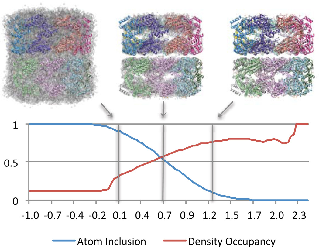
It would be possible to pick a higher threshold to give a higher density occupancy score, however this could mean that a lower atom inclusion score would be obtained at the same threshold (Figure 1). This reduces the possibility of picking thresholds that arbitrarily favor atom inclusion or density occupancy. For the purposes of this paper, we do not attempt to find an optimal threshold that maximizes both scores simultaneously; instead we rely on the thresholds recommended by the authors of the density maps. These thresholds are typically chosen manually such that all densities inside the molecular envelope are included, while background noise densities are not; which in effect tends to balance the atom inclusion and density occupancy scores.

Figure 1.

The top images shows the map of GroEL @4Å resolution (transparent surface), with Segger-docked models (ribbons with different colors for each protein), at 3 thresholds: 0.1, 0.7 and 1.25. The plot shows Atom Inclusion and Density Occupancy scores computed at evenly distributed thresholds for GroEL @4Å resolution, with a Segger-docked model. The threshold at which atom inclusion and density occupancy are balanced in this case is about 0.7 (middle image). The recommended threshold for visualizing this density map, as suggested by the authors of the density map, is 0.8, which is very close to this value.

3.2.4 Clash score

In symmetric maps, a single model can be fit into the map multiple times, with each fit being related by a symmetry operation (e.g. rotation about a symmetry axis). The clash score measures how many clashes occur between atoms in symmetry-related copies of the same model. Two atoms are considered to clash if they are less than 3 Å apart. Low clash scores indicate a better docking result. When the docking results are incorrect, the clash score can be quite high if the copies placed using symmetry operations clash. Thus, the clash score helps to validate the results, because for the correct answer, the clash score should be very low.

If the map is not symmetric and has multiple dissimilar components (for example the ribosome), since we dock only one model at a time, clash scores are not computed. In the present investigation we only compute clash scores in symmetric maps.

3.2.5 The z-score

As previously mentioned, most methods assume the fit with the highest score is the correct one. Unfortunately this criterion is not sufficient to guarantee the correctness of the solution. This begs the need to adopt a statistical score which measures how much the top score stands out above the scores where the structure is arbitrarily docked in the density map. This is reflected in the z-score, which is computed as follows:

$$z=\frac{S_1-\overline{S_{2-N}}}{{\mathrm{\sigma }}_S}$$

In the above, s₁ is the top score, while $\overline{S_{2-N}}$ and σ_s are the mean and standard deviation, respectively, of all other scores found during the docking procedure. The latter, since the search procedure is typically an exhaustive search, are representative of the expected average score obtained if the structure were to be randomly placed in the density map.

The z-score represents how many standard deviations the top score is above the mean. When the z-score is high, it signifies that the fit with the highest score is significantly better compared to the score obtained by randomly placing the structure somewhere else in the map. (Please note that the z-score, also commonly called the standard score in statistics, is different than the Fisher z-transformation, which has also been used in docking to compute confidence intervals²⁰).

Unless optimization is used for each orientation tested, as described in section 3.2, the z-score would be substantially different based on the parameters used during search (e.g. the rotational step size). For example, for smaller step size, the top N scores would include more of the higher scores found around the highest score and thus, the score would be biased towards a higher value. Optimization ensures that scores that are not at local maxima in the fit function are not considered, making the score more invariant to different search parameters. In the results section, we report z-scores for all the scores described in section 3.2: cross-correlation, atom inclusion, density occupancy, and clash scores.

3.3 Comparison of results

3.3.1 Comparison of segmentation results

To compare the three different segmentation methods used in the challenge, we compared the regions produced by each method to models of individual components docked using Segger. When the segmented regions closely match the docked models, it indicates better accuracies in the segmentation. This assumes that the docking results are correct. In the examples presented here, we use the previously published high resolution structures of the macromolecular complex available in the PDB as a guide for the correctness of the docking results.

The results submitted with each method consisted of a separate density map for each segmented region. We visualized each segmented region using Chimera⁸. It appeared to us that different density thresholds and filters were used by each segmentation method. This made the use of a quantitative score for comparing segmentation results difficult, since varying such parameters would significantly affect the score. Thus, we more simply attempted to visually pick a threshold at which the surface of each region representing the same molecular component from different methods appeared roughly the same. In some cases, we also had to manually align the regions from different methods, as they seemed to have been saved with different coordinates and scaling factors. We did not attempt to run the other methods with different parameters, since we did not want to add any bias to the comparison results.

More clearly restricting the use of different coordinate systems, thresholds, and filters in future challenges would allow for a more objective comparison of segmentation results. For this paper we instead rely on a visual comparison of segmentation results. In particular, where the surface of the segmented region is far (>3.0 Å) from atoms in a docked model, it is colored red, and conversely, where atoms in the structure are not closer than 3 Å to any voxel inside the surface of the segmented region, the model is also colored red. This gives a rough sense of where the segmented regions and the docked models disagree.

3.3.2 Validation of docking results

The rigid body docking process typically docks a single molecular component into a density map at a time. If the map represents a macromolecular complex with multiple components, then each component can be docked independently, or one at a time, or all components can be docked simultaneously. When the structure of the entire complex is known, then the entire structure could also be docked into the map rather than breaking it up into individual components. For this paper, we focus on the former, where each component (e.g. a protein chain) is docked independently.

After all components are docked independently, if the structure of the entire complex is known (which is the case for all examples explored in the results section), then all the docked components can be collectively compared to the structure of the entire complex. We do this via an all-atom RMSD score, which is computed as follows:

$$\mathit{\text{RMSD}}=\sqrt{\frac{{\displaystyle \sum _{i=1}^N}{\Vert {\overrightarrow{r}}_i^A-{\overrightarrow{r}}_i^B\Vert }^2}{N}}$$

In the above, ${\overrightarrow{r}}_i^A$ is the position of the i^th of N atoms in a docked model, and ${\overrightarrow{r}}_i^B$ is the corresponding atom in the structure of the entire complex. When multiple models are docked in a density map, it is first necessary to pair each docked model with a particular chain in the structure of the entire complex.

3.3.3 Comparison of docking results

We used the RMSD to compare docking results submitted with different methods, e.g. with MultiFit. Multifit fits multiple components simultaneously, and hence the results typically included a complete macromolecular complex. In the results section, we compare all the models docked with Segger to the structure of the entire complex created with MultiFit, using the all-atom RMSD described in the previous section. The RMSD is computed between atoms in the models docked with Segger and the corresponding atoms in the complex built with MultiFit. Our docking results could not be compared to methods other than MultiFit, such as Gorgon or F2Fit, since the results for these other methods were submitted with atom positions in a different coordinate system; that is, when we opened the models in Chimera, the models did not seem to be inside the corresponding density map which was also opened in the same session.

4. Results

4.1. GroEL @ 4.2Å resolution

This map has D7 symmetry, and the macromolecular complex consists of 14 proteins that span two circular rings of 7 proteins each. The map was segmented with Segger at a threshold of 0.8. After 6 smoothing and grouping steps, 14 regions are obtained which closely match individual proteins. Chain A from the PDB model 1XCK was docked with Segger by aligning it to each of the 14 regions. Rotational search with 100 evenly sampled orientations was used (this is used for all results reported in this paper).

In Figure 2, the top cross-correlation scores obtained while docking just one of the chains to a region are plotted, along with the corresponding atom inclusion, density occupancy, and clash scores. The plots show that the scores for the fit with the highest cross-correlation score stand out quite significantly above the other scores computed during the search. The high z-scores also reflect this (Table 1). The z-score for the clash scores is negative since the fit with the highest cross-correlation also has a clash score that is below the mean.

Figure 2.

Top 9 scores obtained while docking PDB:1XCK chain A into the density map of GroEL at 4.2Å resolution (EMDB: 5001) using Segger. The plots show that for all scores (cross-correlation, density occupancy, and clash score), the fit wit the top score has a significantly higher score than the next 8 top scores, which represent an incorrect or random placement of the structure in the density map.

Table 1.

Docking scores the GroEL 4.2Å resolution map.

PDB:1XCK chain A (65 unique fits found)
Score	z-score	Top score	Mean	STDev
Cross-correlation	21.59	0.48	0.31	0.008
Atom Inclusion	27.65	0.40	0.20	0.007
Density occupancy	23.42	0.69	0.27	0.018
Clash score	−2.16	0.02	0.17	0.070

The all-atom RMSD between the 14 docked models and the crystal structure of the entire complex (PDB:1XCK) was very low, 1.52 Å, showing that the docking results are consistent with the crystal structure. The all-atom RMSD between the Segger-docked models and the results submitted with Multifit was 4.39, meaning the two docking results are also similar.

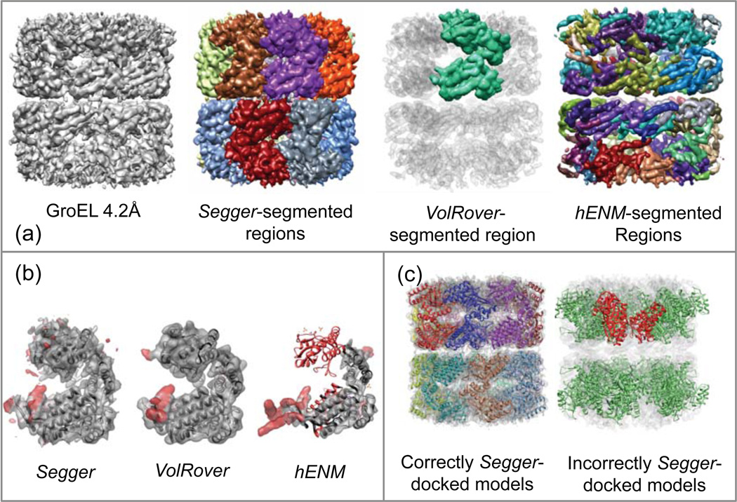
The segmented regions submitted to the challenge are shown in Figure 3a and the comparison of segmented regions to the docked model of a single subunit is shown in Figure 3b. The results submitted for VolRover was a single “average” region corresponding to one of the 14 proteins. As Figure 3b shows, both Segger and VolRover produced regions that quite closely match the docked structure, except for some red areas on the surface around the equatorial region. The submitted results for hENM include 62 regions, none of which seem to match any of the docked structures. One of the hENM regions is also compared to a docked model, and it can be seen in the figure that it only partially matches the docked model of a single subunit.

Figure 3.

(a) Density map and segmentation results for GroEL at 4.2Å resolution (EMDB:5001). (b) Segmented regions (transparent surfaces) from Segger, VolRover, and hENM is compared to the Segger-docked model (PDB:1XCK chain A). Red coloration signifies disagreement. (c) All 14 docked models of the same chain (random-colored ribbons) docked inside the density map (transparent surface), and an incorrectly docked model (red ribbon) along with symmetric copies (green ribbon) inside the map.

Figure 3c shows the incorrectly and correctly docked models using Segger in the same density map. To produce the incorrect docked models for illustration purpose, we first picked at random one of the fits produced by Segger (of course excluding the fit with the highest cross-correlation score, which is the correct fit in this case). The model was then copied 13 times using the D7 symmetry operation for this complex. Taken collectively, they have an all-atom RMSD of 42.12 when compared to the original crystal structure. Thus, the RMSD score is very high when docking results are inconsistent with the known crystal structure.

4.2. GroEL+GroES @ 7.7Å resolution

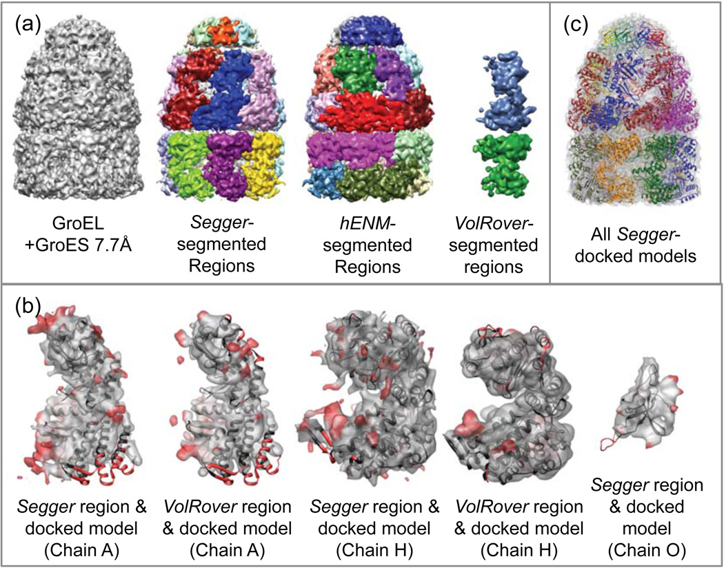
The GroEL+GroES complex has C7 symmetry and consists of 21 proteins, or 3 stacked circular rings of 7 proteins each (Figure 4a). The map was segmented at a threshold of 0.5 with Segger. After 4 smoothing and grouping steps, single regions were obtained for each protein in the lid (GroES section), and 2 regions were obtained for each of the proteins in the barrel (GroEL section). Further smoothing and grouping results in regions corresponding to different proteins joining, which is why the process was stopped after 4 steps. Regions corresponding to the same protein were then joined interactively in the GroEL section.

Figure 4.

(a) Density map and segmentation results for GroEL+GroES at 7.7Å resolution (EMDB:1180). (b) Comparison of segmented regions from Segger and VolRover and docked models. (c) All Segger-docked models inside the density map.

Chains A, H (corresponding to proteins in the GroEL top and bottom rings respectively), and O (corresponding to proteins in the GroES ring) from the structure PDB:2C7C were docked with Segger to single regions corresponding to each of the 3 different proteins in the map in Figure 4b. The z-scores for chains A and H were modest, between 7 and 10 (Table 2), and for chain O, which is a much smaller protein, they were quite low (<4). The 7 proteins in each ring were aligned jointly to the corresponding ring in the crystal structure. The all-atom RMSDs for each of the rings were very low (chain A:2.4, H:1.23, O:1.49) signifying that the docking results are correct. All-atom RMSD scores between Segger and Multifit results, computed for each ring, are also low (A:1.7, H:0.89, O:3.42) showing the two methods are in agreement.

Table 2.

Docking scores for GroEL+GroES @ 7.7Å resolution.

PDB:2C7C chain A (37 unique fits found)
Score	z-score	Top score	Mean	STDev
Cross-correlation	7.81	0.79	0.67	0.015
Atom Inclusion	8.76	0.83	0.61	0.025
Density occupancy	7.57	0.38	0.29	0.012
Clash score	−1.06	0.02	0.10	0.074
PDB:2C7C chain H (37 unique fits found)
Cross-correlation	9.31	0.82	0.69	0.013
Atom Inclusion	7.86	0.82	0.64	0.022
Density occupancy	8.36	0.40	0.30	0.012
Clash score	−1.40	0.02	0.07	0.042
PDB:2C7C chain O (27 unique fits found)
Cross-correlation	4.29	0.79	0.72	0.016
Atom Inclusion	1.82	0.82	0.75	0.041
Density occupancy	2.83	0.39	0.34	0.018
Clash score	−0.99	0.15	0.26	0.109

The segmented regions and docked models are shown in Figure 4a,c. The results by VolRover include 2 regions, each one corresponding to a single protein in the top and bottom rings of the GroEL. Submitted VolRover results did not include a region corresponding to the protein in the lid section (GroES). Both Segger and VolRover produce regions in individual chains that are quite similar to the docked structures, aside from a few small red areas (Figure 4b ?). The results submitted for hENM include 24 regions (figure 4a). None of the segmented regions seemed to match any docked models closely and hence no comparison is shown in Figure 4.

4.3. GroEL+GroES @ 23.5Å resolution

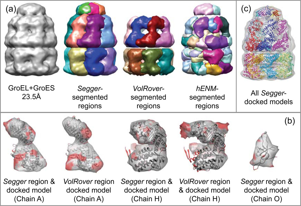
This map was segmented at a threshold of 0.06 with Segger. After 3 smoothing and grouping steps, single regions were obtained for each protein in the lid (GroES section), and 2 regions corresponded to each protein in the barrel (GroEL section). Regions corresponding to the same protein were then joined interactively.

Chains A, H and O from PDB:2C7C were docked into the map to corresponding regions using Segger. The z-scores were very low (<5) for all chains, most likely due to the low resolution of the map (Table 3). However all-atom RMSD scores between docked models and the crystal structure (here computed for each ring rather than the entire complex) were reasonable (A:5.07, H:3.06, O:6.03) for this resolution map, showing the docked results are quite close to the crystal structure. All-atom RMSD scores between Segger and Multifit results were also low (A:2.49, H:3.15, O:6.24).

Table 3.

Docking scores for GroEL+GroES @ 23.5Å resolution.

PDB:1GRU chain A (7 unique fits found)
Score	z-score	Top score	Mean	STDev
Cross-correlation	5.65	0.94	0.76	0.032
Atom Inclusion	1.83	0.99	0.81	0.102
Density occupancy	3.98	0.68	0.46	0.055
Clash score	−1.18	0.03	0.23	0.171
PDB:1GRU chain H (7 unique fits found)
Cross-correlation	2.59	0.93	0.85	0.032
Atom Inclusion	1.87	0.99	0.92	0.038
Density occupancy	1.98	0.55	0.46	0.045
Clash score	−1.20	0.10	0.34	0.203
PDB:1GRU chain O (7 unique fits found)
Cross-correlation	2.59	0.93	0.85	0.032
Atom Inclusion	1.87	0.99	0.92	0.038
Density occupancy	1.98	0.55	0.46	0.045
Clash score	−1.20	0.10	0.34	0.203

The segmented regions and their comparison to the docked models are shown in Figure 5a–b. VolRover results included one region per protein in the barrel (GroEL section), but no regions for the lid (GroES section). Results with hENM show 83 regions, which somewhat follow the protein boundaries, but single regions were not obtained for each protein. Again, both VolRover and Segger regions are very close to the docked models (Figure 5c).

Figure 5.

(a) Density maps and segmentation results for GroEL at 23.5Å resolution (EMDB 1046). (b) Comparison of segmented regions from Segger and Volrover and the docked models. (c) All Segger-docked models inside the density map.

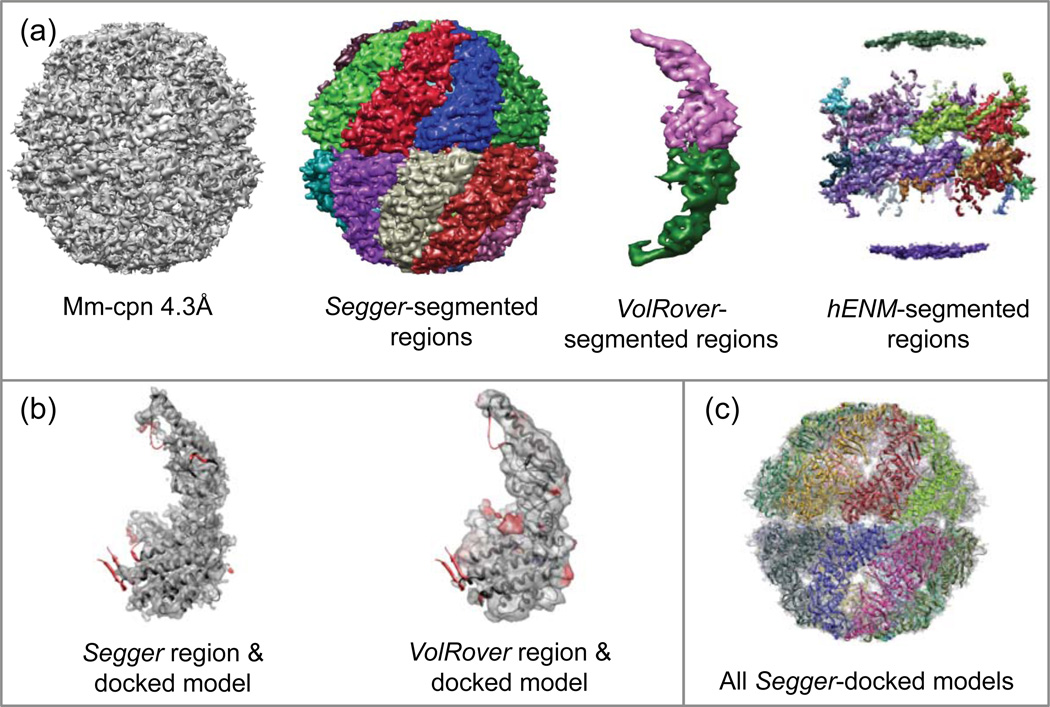
4.4. Mm-cpn @ 4.3Å resolution

This map has D8 symmetry and it represents an assembly with 16 proteins, which are arranged in two rings of 8 proteins each. The map was segmented at a threshold of 0.3. A total of 6 smoothing and grouping steps were performed to obtain 48 regions, or 3 regions for each of the 16 proteins. The 3 regions corresponding to each chain were then grouped interactively.

Chain A of the crystal structure PDB:3KFB was docked into the map by aligning it to each of the regions. The z-scores were very high, between 15 and 30 (Table 4). The all-atom RMSD scores between the docked models and the crystal structure was very low (1.56), and the RMSD score between the Segger docked models and the submitted Multifit result was 3.68.

Table 4.

Docking scores for Mm-cpn @4.2Å resolution.

PDB:3KFB chain A (73 unique fits found)
	z-score	Top score	Mean	STDev
Cross-correlation	27.73	0.61	0.44	0.006
Atom Inclusion	15.81	0.43	0.23	0.013
Density occupancy	26.45	0.51	0.25	0.010
Clash score	−2.65	0.02	0.27	0.093

The segmented regions and their comparison to the docked models are shown in Figure 6a–b. The submitted results created by VolRover consisted of 2 regions for proteins in the top and bottom half of the assembly. Submitted results for hENM consisted of 18 regions, which not only seemed to have been segmented at too high of a threshold, but also didn’t quite capture the shape of any of the proteins. The segmented regions produced by Segger and VolRover on the other hand quite closely match the docked models.

Figure 6.

(a) Density map and segmentation results for Mm-cpn at 4.3Å resolution (EMDB:5001). (b) Comparison of segmented regions from Segger and Volrover and the docked models. (c) All Segger-docked models inside the density map.

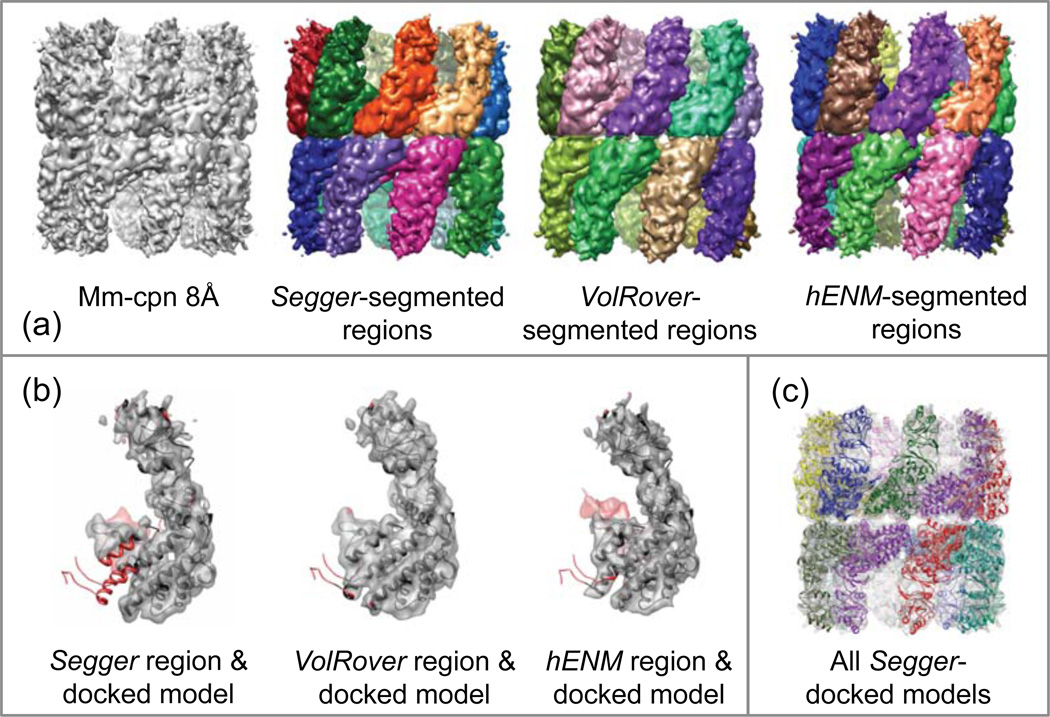
4.5 Mm-cpn @ 8Å resolution

This map has D8 symmetry, and represents the assembly with 16 proteins in an open state. It was segmented at a threshold of 0.9 with Segger. A total of 11 smoothing and grouping steps were performed to obtain 16 regions, each region corresponding to a single protein. Single regions per protein are produced in this map without the need for interactive grouping since the proteins are more separated in this open state than in the closed state (Mm-cpn at 4.3Å resolution)

Chain A of the structure PDB:3KFK was docked into the map with Segger by aligning it to one of the regions. The z-scores were moderately high, being between 8 and 12 (Table 5). The all-atom RMSD between Segger docked models and the entire crystal structure is very low (2.43), and that between Segger and the submitted Multifit results are also quite low (2.59).

Table 5.

Docking scores for Mm-cpn @8Å resolution.

PDB:3KFK chain A (36 unique fits found)
	z-score	Top score	Mean	STDev
Cross-correlation	8.78	0.68	0.51	0.019
Atom Inclusion	7.51	0.47	0.29	0.024
Density occupancy	11.30	0.52	0.29	0.020
Clash score	−0.68	0.01	0.13	0.175

Figure 7a–c shows the segmented regions submitted with each method, all models docked with Segger, and the comparison between regions and docked models. For this map, all methods produce single regions for each protein, which are also quite close to the docked models. This may have been the easiest maps to segment, since there is substantial separation between each protein on all sides except where the proteins connect in the equatorial section.

Figure 7.

(a) Segmentation and results for Mm-cpn at 8Å resolution (EMDB:5140). (b) Comparison of segmented regions from Segger and VolRover and Segger-docked models. (c) All Segger-docked models inside the density map.

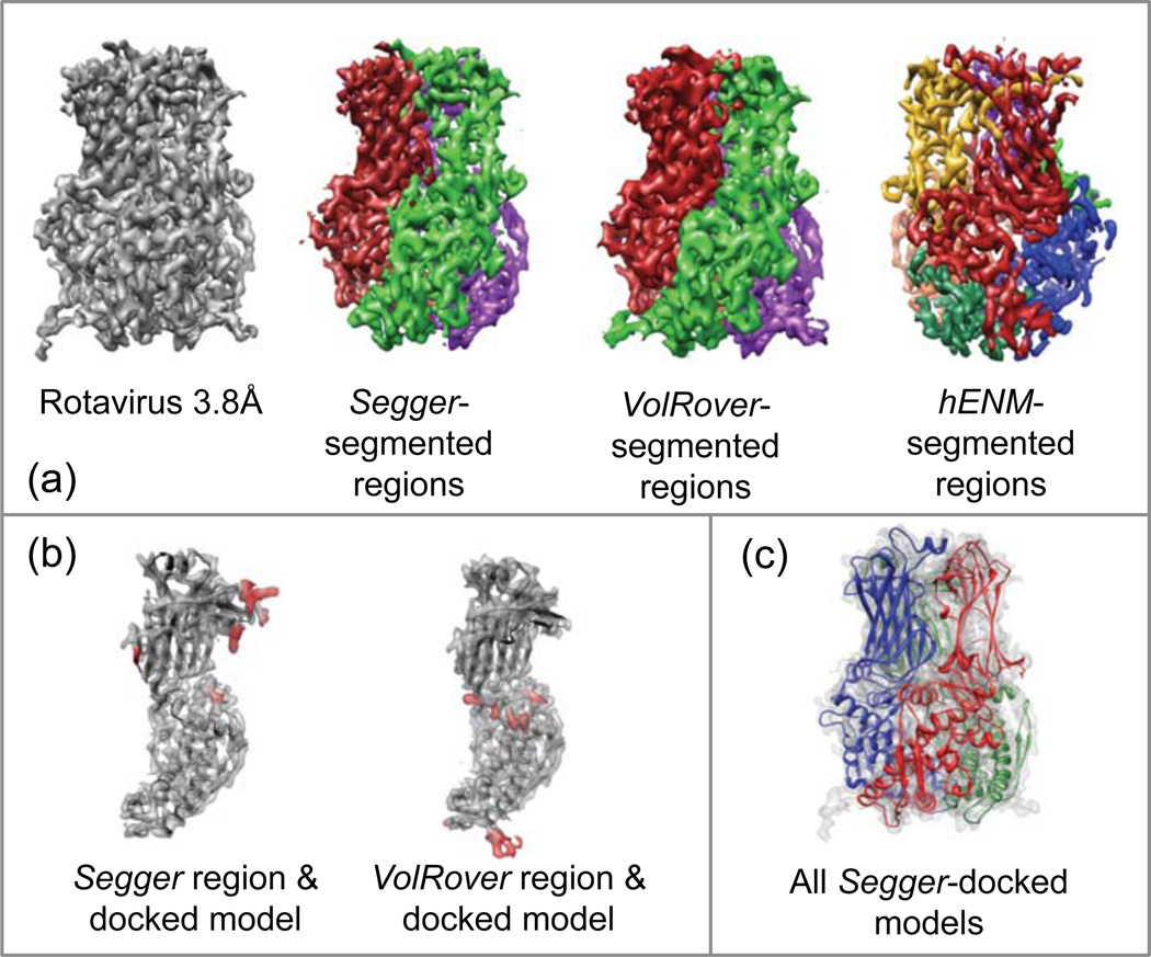
4.6. Rotavirus VP6 protein @ 3.8Å resolution

Rotavirus is an incosahedral complex with 6, 3, and 2-fold symmetry. This map shows the 3-fold arrangement of the VP6 protein in one of the capsid shell. The map was segmented at a threshold of 1.04. A total of 4 smoothing and grouping steps were performed after which 4 regions were interactively joined to form larger regions corresponding to each of the 3 proteins.

The structure PDB:1QHD was docked into the map with Segger by aligning it to one of the 3 regions. The z-scores were quite high, being between 12 and 34 (Table 6). The all-atom RMSD score between all 3 docked chains and the complete crystal structure is very low (0.39), meaning the docking recreate the structure of the complex as seen in the crystal structure. Results with Multifit were not submitted for this structure, and as in all other cases, the results submitted with F2Fit and Gorgon appeared to have been saved in different coordinate systems.

Table 6.

Docking scores for Rotavirus @3.8Å resolution.

PDB:1QHD (34 unique fits)
	z-score	Top score	Mean	STDev
Cross-correlation	12.18	0.57	0.38	0.016
Atom Inclusion	33.31	0.36	0.11	0.008
Density occupancy	17.51	0.76	0.29	0.027
Clash score	−2.48	0.14	0.45	0.125

Figure 8a–c shows the segmented regions and also the comparison between the regions from each method and one of the docked models. Results submitted with VolRover also consisted of 3 regions, and results with hENM include 7 regions, as shown in Figure 8a. A hENM region was not compared to the docked model since none of the regions seemed to closely match it.

Figure 8.

(a) Density map and segmentation results for the rotavirus density map @3.8Å resolution (EMDB:1461). (b) Comparison between segmented regions and Segger-docked models. (c) All 3 Segger-docked models in the density map.

4.7. Epsilon 15 Phage @ 4.5Å Resolution

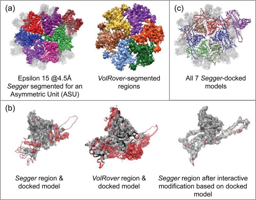
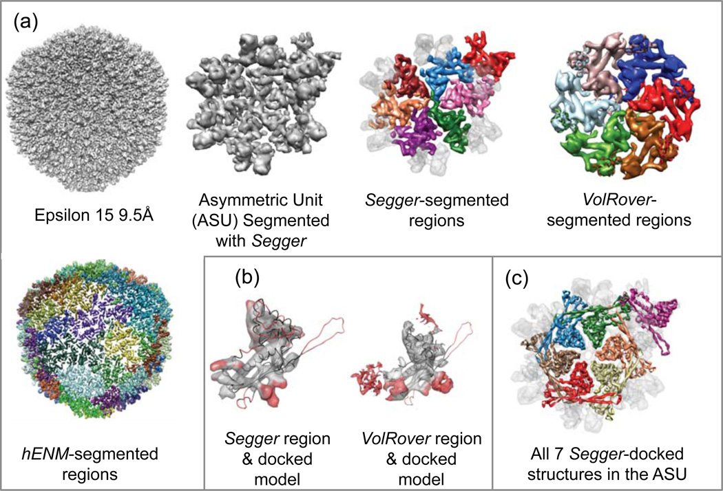
This map captures the structure of a virus capsid with icosahedral symmetry. It consists of 6, 5, 3 and 2-fold symmetrically arranged proteins. Two type of proteins are known to be present in the capsid: gp7 and gp10²¹. A sub-region of the map containing an asymmetric unit was first cropped out to make segmentation easier, since the entire map is quite large (768³ voxels). The cropped map was segmented at a threshold of 0.004. A total of 4 smoothing and grouping steps were then performed, after which 4 regions were interactively joined to form larger regions corresponding to individual proteins in an asymmetric unit. Regions corresponding to both gp7 and gp10 proteins were segmented (Figure 9a).

Figure 9.

(a) Segmentation esults for Epsilon 15 @ 4.5Å resolution (EMDB:5003). (b) Comparison of Segger and VolRover regions and one of the docked models, and a Segger region after interactive modification based on the docked model. (c) All 7 Segger-docked models inside the asymmetric unit.

While crystal structures are not available for gp7 or gp10 proteins, a model of the asymmetric unit was built based on this map (PDB:3C5B). In this model of one asymmetric unit, each chain has the same sequence, however each chain has a slightly different conformation (chain to chain RMSD is ~1Å). Hence, each of the 7 chains from the structure 3C5B was docked independently into the map using Segger by aligning them to the corresponding region. The z-scores computed for chain A are shown in Table 7, and were very high. An all-atom RMSD score between the 7 docked models and the original structure 0.82, showing the docking results are consistent with the original structure.

Table 7.

Docking scores for Epsilon 15 @4.5Å resolution.

PDB:3C5B chain A (89 unique fits)
	z-score	Top score	Mean	STDev
Cross-correlation	20.29	0.57	0.37	0.010
Atom Inclusion	17.38	0.83	0.37	0.026
Density occupancy	23.19	0.25	0.11	0.006
Clash score	−2.44	0.01	0.12	0.045

Figure 9a–c shows the segmented regions for Segger and VolRover, and a comparison between one of the regions and a docked model. No results were submitted with hENM. Both Segger and VolRover results incorrectly segmented the long protruding loop in this structure, which closely interacts with a neighboring protein (Figure 9b). Although it would be possible to interactively regroup regions with Segger to properly segment the loop, we did not do that for these results. The region produced by VolRover seems to have slightly more areas far from the structure in this case, though most of this can be attributed to the gp10, which was not segmented out with VolRover.

Figure 9b also shows the Segger region corresponding to a docked model after small segments from the adjacent region were ungrouped and regrouped interactively, so that the protruding loop is assigned to the correct region. In this way, the segmentation can be refined using the Segger interface based on docked models. This is an interesting case that a fully automated segmentation procedure cannot unambiguously resolve the protruding loop as which subunit it belongs even in a 4.5 Å map because it extends to its neighboring component quite closely. In the original paper²¹, the segmentation was achieved manually and iteratively during the de novo modeling process. In addition, the structural fold from homologous structures that the loop would exist helps to decide how to segment the protruding loop.

4.8. Epsilon 15 Phage @ 7.3 Å Resolution

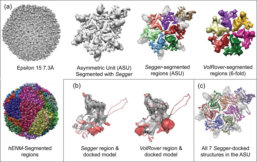
This map was segmented with Segger at a threshold of 1.6. Since this map has lower grid size than the higher resolution map, and DNA densities are not included at this threshold, cropping was not needed to speed up the segmentation process. A total of 3 smoothing and grouping steps were performed, after which 2 regions were interactively joined to form larger regions corresponding to individual gp7 proteins in the asymmetric unit (Figure 10a). Regions corresponding to the gp10 dimers which sit on top of the gp7 proteins could also be seen and were segmented (transparent regions in Figure 10a).

Figure 10.

(a) Density map and segmentation results for Epsilon 15 @ 7.3Å resolution (EMDB:1557). (b) Comparisons of Segger and VolRover regions to one of the docked models. (c) All 7 Segger-docked models inside the asymmetric unit.

A single chain from the structure PDB: 3C5B was docked into the map with Segger by aligning it to each of the 7 regions corresponding to the gp7 proteins in the asymmetric unit. The z-scores were moderately high for all scores (Table 8). The all-atom RMSD between all 7 docked models and the original structure was computed to be 4.41, showing the docking results are consistent. This score is considerably worse than that computed for Epsilon 15 at 4.5 Å resolution simply because this structure does not fit the map as perfectly as it fits the map it was built based on. No other rigid body docking results were submitted for this target.

Table 8.

Docking scores for Epsilon 15 @7.3Å resolution.

PDB:3C5B chain A (56 unique fits)
	z-score	Top score	Mean	STDev
Cross-correlation	26.08	0.68	0.50	0.007
Atom Inclusion	10.86	0.70	0.45	0.024
Density occupancy	5.78	0.81	0.65	0.029
Clash score	−2.67	0.01	0.17	0.060

Figure 10a–c shows the map and all segmented regions produced with Segger or submitted to the challenge with VolRover and hENM. It also shows all 7 docked models, and the comparison between Segger and VolRover regions and a docked model. Again the long protruding loop is not segmented correctly for this map. Segmentation results with hENM included 105 regions spanning the entire map, but none seemed to correspond to individual proteins (Figure 10b).

4.9. Epsilon 15 Phage @ 9.5Å Resolution

The entire map was segmented with Segger at a threshold of 1.6. Then, 5 smoothing and grouping steps were performed, after which 2 regions were interactively joined to form larger regions corresponding to individual gp7 proteins in an asymmetric unit. Regions corresponding to the gp10 proteins were again seen and segmented. As reported in the original paper, gp10 was not known to exist and this density was mis-interpreted as part of the gp7²². It is interesting to note that even the density can be resolved and segmented, one would not be able to make proper annotation to the observed density if no other biochemical information was available in this case.

A single protein chain from the structure PDB:3C5B was docked into the map with Segger by aligning it to one of the 7 regions in the asymmetric unit corresponding to the gp7 protein. The z-scores were again moderately high (Table 9). The all-atom RMSD score between all 7 docked models and the original structure was computed to be 4.57, showing the docking results are consistent. No other rigid body docking results were submitted for this target.

Table 9.

Docking scores for Epsilon 15 @9.5Å resolution.

PDB:3C5B chain A (53 unique fits)
Score	z-score	Top score	Mean	STDev
Cross-correlation	14.52	0.63	0.47	0.011
Atom Inclusion	6.61	0.56	0.33	0.034
Density occupancy	16.33	0.63	0.40	0.014
Clash score	−2.43	0.02	0.19	0.070

Figure 11 shows the segmentation and docking results. Segmented regions produced by Segger and VolRover again match the docked model reasonably well, although again the long protruding segment is not captured correctly. Results with hENM consisted of 35 regions, but again none seemed to closely correspond to individual proteins.

Figure 11.

(a) Density map and segmentation results for Epsilon 15 @ 9.5Å resolution (EMDB:1176). (b) Comparisons of Segger and VolRover regions to docked models. (c) All 7 Segger-docked models inside the asymmetric unit.

4.10. Ribosome @ 7.4 Å resolution

This map which captures an 80S ribosome was segmented with Segger at a threshold of 0.5. A total of 5 smoothing and grouping steps (initial filter width 5 voxels) were performed, after which the two resulting regions corresponded to the large and small ribosome subunits.

Models have been built based on this density map which includes the large subunit PDB: PDB:3JYW and PDB:3JYX, and the small subunit PDB:3JYV. We first docked each subunit into the map separately by aligning each to the corresponding region. Rotational search with 121 evenly sampled orientations was used. The z-scores were very high for both subunits (see Table 10). The all-atom RMSD computed between the docked structures and the original structure was very low (0.4), meaning the docking results are consistent.

Table 10.

Docking scores for Ribosome @7.4Å resolution.

PDB:3JYW and 3JYX (98 unique fits)
Score	z-score	Top score	Mean	STDev
Cross-correlation	25.03	0.64	0.51	0.005
Atom Inclusion	21.91	0.46	0.31	0.007
Density occupancy	3.36	0.07	0.06	0.003
PDB:3JYV (74 unique fits)
Cross-correlation	31.93	0.66	0.50	0.005
Atom Inclusion	23.15	0.49	0.31	0.008
Density occupancy	1.69	0.06	0.05	0.005
PDB:2GO5 chain 4 (32 unique fits)
Cross-correlation	11.50	0.68	0.58	0.009
Atom Inclusion	5.79	0.36	0.29	0.011
Density occupancy	9.40	0.69	0.48	0.022
PDB:2GO5 chain 5 (11 unique fits)
Cross-correlation	2.05	0.80	0.66	0.070
Atom Inclusion	2.29	0.58	0.42	0.073
Density occupancy	2.51	0.59	0.39	0.079

A target structure for segmentation for this map, set by the challenge, is PDB:2GO5. This structure was built based on this map by docking known and homology based structures into the map²³. It consists of 6 proteins and 3 RNA chains. To segment out these structures using Segger without other structural knowledge would be very challenging, since regions produced by Segger after smoothing and grouping do not directly correspond to individual molecular components. Segmenting out RNA components is particularly challenging since they can be long and have proteins closely connected in multiple locations.

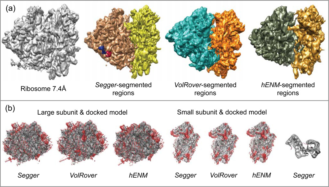
Here we attempted to segment out just two of the proteins, chains 4 and 5 in PDB:2GO5. This was meant as an illustrative process, and we didn’t segment out other regions to keep the results section of reasonable length. For guidance in trying to segment out these proteins, we looked at the positions of chains 4 and 5 in the PDB model, which already has these proteins docked in their correct locations in the map. The map was re-segmented with Segger to try to extract corresponding regions, using only 1 smoothing step at the default initial width of 1 voxel. Six of the resulting regions were interactively grouped to produce a single region for chain 4, and 7 regions were interactively grouped to produce a single region for chain 5 (Figure 12). Smoothing and grouping further would have resulted in these regions joining incorrectly into other regions. The fact that so many regions have to be interactively joined together reflects the inability of any of the current software in properly segmenting out proteins in a ribosome without other information about the location of the protein components in the complex.

Figure 12.

(a) Density map and segmentation results for Ribosome at 7.4Å resolution (EMDB:1217). (b) Comparisons between segmented regions and the Segger-docked models. The first three images from the left show segmented regions and the large subunit (PDB:3JYW & 3JYX). The second three image show regions and the small subunit (PDB:3JYV). The rightmost image shows Segger regions and the docked models for PDB:2GO5 chains 4 and 5.

The two chains in this structure PDB:2GO5 were then docked individually using Segger, using each corresponding region as a guide. The z-scores were moderately high for chain 4 (see Table 10), however they were quite low for chain 5, potentially due the smaller size of this model compared to the larger chain 4. All-atom RMSD between docked models and the corresponding models in the original structure were all very low (large subunit: 2.8, small-subunit:2.9, chain 4:1.5, and chain 5:1.5). Note that here we did not jointly compute an RMSD between all docked models and the structure of the entire complex, since we did not dock all the sub components of the complex. Instead, since all the structures were already previously docked into the density map and are provided as such, we just computed the all-atom RMSD between our docked models, as placed, and the corresponding components in the original structures, to test whether our docking results match the previous docking results.

The segmentation and docking results are shown in Figure 12. Segmented regions submitted with VolRover and hENM also separated out the large and small subunits, and comparison to docked models show that regions produced by all three segmentation methods match the docked models quite well. (Note that the map submitted with hENM had to have the y-coordinate flipped and the pixel spacing parameter multiplied by 3.5 in order to make it agree with the docked models and original map). The regions produced with Segger for chains 4 and 5 also compare well with the docked models. VolRover and hENM did not submit other regions for proteins or other RNA.

4.11. Ribosome at 8.9Å resolution

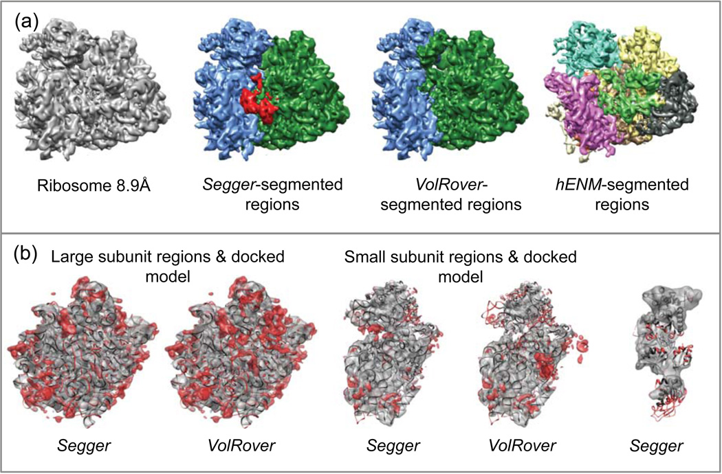
The map was segmented at a threshold of 45. A total of 3 smoothing and grouping steps (initial filter width of 5 voxels) were performed, after which 3 regions were obtained. Two regions corresponding to the small subunit were joined interactively, to produce two regions corresponding to the small and large subunits (Figure 13a).

Figure 13.

(a) Density map and segmentation results for Ribosome at 8.9Å resolution (EMDB:1345). (b) Comparisons between regions and the Segger-docked models. The first two images from the left show segmented regions and the large subunit (PDB:3JYW & 3JYX). The second two image show regions and the small subunit (PDB:3JYV). The rightmost image shows a Segger region and the docked model PDB:2P8W.

Structural models have been built for this map based on homology models, including proteins and RNA and in the large and small subunit (PDB:3JYV, 3JYW, 3JYX), and elongation factor (PDB:2P8W)²⁴. Again segmenting out each protein and the RNA interactively would be a challenge, and Segger does not produce single regions for each component. Here we aim to segment out one of the larger proteins, the elongation factor protein (PDB:2P8W) with Segger, based on the structural knowledge provided by the previously docked model. The coordinates in the PDB file already represent the model docked in its appropriate position in the density map. We re-segmented the map with Segger to try to extract a corresponding region; 3 smoothing steps were used at the default initial width of 1 voxel. Four of the regions overlapped the docked protein, which were joined interactively.

The models PDB:3JYW and PDB:3JYX, which contain proteins and RNA making up the large subunit, were jointly fit into the map using Segger, by aligning them to the region corresponding to the large subunit. Rotational search with 121 evenly sampled orientations was used. The model PDB:2P8W was also docked by aligning it with the corresponding segmented region. The z-scores were moderately high (Table 11). All-atom RMSD scores between docked models and the corresponding models in the original structure were all very low (large subunit: 2.4, small-subunit:2.5, PDB:2P8W:1.7) signifying the docking results are consistent.

Table 11.

Docking scores for Ribosome @8.9Å resolution.

PDB:3JYW and 3JYX (76 unique fits)
Score	z-score	Top score	Mean	STDev
Cross-correlation	14.29	0.59	0.49	0.007
Atom Inclusion	28.96	0.48	0.21	0.009
Density occupancy	8.75	0.45	0.42	0.003
PDB:3JYV (32 unique fits)
Cross-correlation	11.67	0.68	0.61	0.006
Atom Inclusion	8.89	0.51	0.43	0.009
Density occupancy	5.71	0.47	0.43	0.007
PDB:2P8W (27 unique fits)
Cross-correlation	18.89	0.73	0.56	0.009
Atom Inclusion	6.30	0.41	0.34	0.011
Density occupancy	5.16	0.48	0.32	0.031

The segmentation and docking results are shown in Figure 13a–b. The submitted VolRover results included 2 regions, or one region per large and small subunit, as shown. hENM results included 10 regions, which didn’t appear to correspond to either subunits. The Segger and VolRover regions match the docked models for the small and large subunits quite closely. The Segger region corresponding to the model 2P8W also matched the docked model quite well.

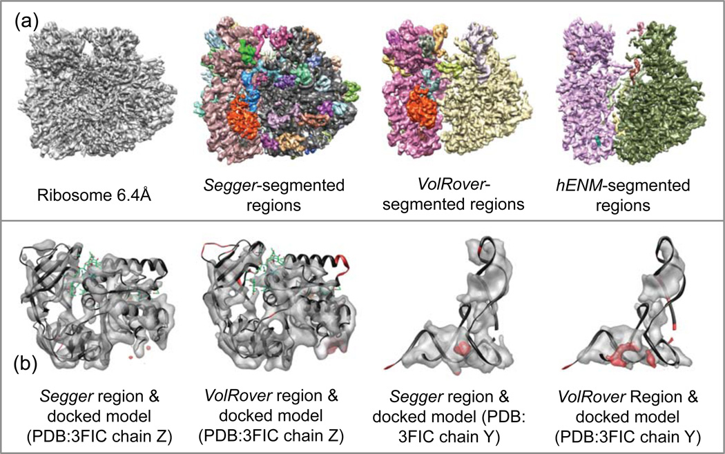
4.12. Ribosome @ 6.4 Å resolution

This map represents the Thermus thermophilus ribosome. A structural model was built based on it using homology models (PDB:3FIC and 3FIN), which include 33 proteins and 37 separate RNA chains²⁵. In this case, we attempted to build regions for all proteins and RNA chains; however to do so interactively would be challenging, as shown in the previous sections. Thus we again used the already docked models in the structures PDB:3FIC and 3FIN for guidance. First, the map was segmented at a threshold of 3.0, and then two smoothing and grouping steps (initial filter width of 5 voxels) were performed. The regions that overlapped each protein were automatically joined to produce regions corresponding to proteins, using a script that detects atoms and region overlaps. The regions that overlapped RNA in each of the large and small subunits were also automatically joined (Figure 14a).

Figure 14.

(a) Density map and segmentation results for Ribosome at 6.4Å resolution (EMDB:5030). (b) Comparisons between regions produced with Segger and VolRover compared to Segger-docked models.

Two of the 33 proteins in the initial structure were then docked by alignment to the corresponding regions, to test our docking method in this scenario. We only explored docking results for two proteins to keep the results section of reasonable length. We picked these two proteins in particular since segmented regions were also submitted by VolRover, and hence a comparison between Segger and VolRover can be made. The models for 3FIC chains Y and Z were docked by alignment to their corresponding regions. The z scores were quite high (Table 12) and the all-atom RMSDs between the docked models and the models in the original structure were low (1.6 and 2.3), signifying that indeed the docking results correspond well to the initial structure.

Table 12.

Docking scores for Ribosome @6.4Å resolution.

PDB:3FIC chain Y (30 unique fits)
Score	z-score	Top score	Mean	STDev
Cross-correlation	6.94	0.72	0.48	0.035
Atom Inclusion	8.50	0.56	0.25	0.036
Density occupancy	12.43	0.61	0.39	0.018
PDB:3FIC chain Z (52 unique fits)
Cross-correlation	28.16	0.63	0.46	0.006
Atom Inclusion	29.47	0.34	0.20	0.005
Density occupancy	20.94	0.68	0.36	0.016

Figure 14a shows the segmentation and docking results. Segmentation regions submitted for VolRover also included two regions for the RNA in the large and small subunits, and several smaller regions for proteins and other RNA molecules. Results submitted with hENM were also similar, with two large regions, and several smaller regions that in this case did not seem to correspond to any proteins. Regions corresponding to the models 3FIC chains Z and Y were found in the VolRover results, and in Figure 14b they are compared along with Segger regions to the docked models. Both methods produced regions that quite closely match the docked models.

5. Discussion and conclusions

We have presented segementation and rigid-body docking methods implemented by Segger, and applied them to the density maps that were part of the 2010 cryo-EM challenge. We compared our results with other results submitted to the challenge in the segmentation and rigid body docking categories.

For segmentation, Segger was used to produce regions that matched individual molecular components reasonably well. In some cases, e.g. GroEL @4.2Å resolution and Mm-cpn @8Å resolution, Segger produced single regions corresponding to individual protein components without much manual intervention aside from the smoothing and grouping process. This could be attributed to the fact that proteins in these complexes have quite a bit of space around them, i.e. they are not very tightly packed, hence allowing the smoothing and grouping process to produce regions that corresponded to individual components. However in other cases, where molecular components are more tightly packed against each other, the smoothing and grouping process did not produce the right grouping, and some user guidance was required to group regions corresponding to individual components. The toughest maps to segment were the ribosome maps in particular, where proteins are closely packed against long chains of RNA; in these maps however, the large and small subunits were segmented out quite easily by the smoothing and grouping process.

One of the challenges in segmentation with Segger is deciding which regions make up a single protein component in a multi-protein complex. For example, Segger shows a clear segmentation of the regions corresponding to the two protein components (gp7 and gp10) in a 9.5 Å map of the Epsilon15 phage. However, without further knowledge about the composition of the phage shell, i.e. that there indeed two different types of proteins, it would be very difficult to know from the segmentation alone whether these regions are part of the same protein or not; further smoothing and grouping would join the two regions together. This example elucidates the challenge in the interpretation of the segmented results in cryo-EM map even at subnanometer resolutions. The user still has to make a correct interpretation of the results based on knowledge of the biochemical composition of the complex being analyzed.

The docking results produced by Segger were all found to be consistent with known structures, as shown by low RMSD. We described the use of 4 scores to assess docking results: cross-correlation, atom inclusion, density occupancy, and clashes with symmetry-related copies. These scores alone are hard to interpret, as they vary greatly from map to map and model to model, and are also influenced by various parameters, e.g. thresholds. Thus we also computed z-scores for each of the 4 scores. These provide a quantitative measure indicating whether the peak score is significantly higher than other peaks in the scoring function, and thus whether the docking result is significant in a statistical sense. Such a quantitative measure would be useful when the target docking results are not known ahead of time, as they were here. The z-scores tended to be high in higher resolution maps, and low in lower resolution maps (e.g. GroEL @23Å resolution) or when docking smaller proteins. This seems to match intuition, since for example, when docking models into lower resolution maps or when docking smaller models, scores tend to be more similar for different positions and orientations.

When comparing segmented regions to docked models, Segger and VolRover produced very similar regions that roughly matched the models. However, both methods tend to segment narrow protruding segments incorrectly, for example in the case of the Epsilon 15 phage subunit. Segmented regions produced by hENM varied more considerably in reliability, and in a lot of cases they did not correspond to individual components. This may be because hENM is the least subjective amongst the three methods, and seems to require the least input from the user. On the other hand, Segger depends on some direction from the user, and VolRover requires ‘seeds’ to be provided as input, where seeds are points inside each component to be segmented.

When using Segger, the smoothing and grouping process does not always correctly join regions. This can be overcome with some user guidance, however in this case the user could potentially create incorrect segmentations. Fully automated and objective segmentation of molecular components in density maps thus remains a challenge. In particular, long protruding segments closely situated to the neighboring subunit are typically hard to segment properly. For example, in the case of the Epsilon15 phage, neither Segger nor other software was able to decide by itself which subunit the long protruding segment belongs to, even in the 4.5 Å resolution map. Such decisions thus remain to be made during the modeling of the protein component and with the knowledge of the fold of a homolog protein.

The docking method used by Segger relies on the segmentation process producing regions that match the models being docked. If incorrect segmentation results are used to guide the docking process, it is very possible that the docking results will also be incorrect. In our experience, this is reflected in low z-scores, i.e. low statistical significance of docking results. In such cases, the segmentation can be modified and docking attempted again. It is also very possible that the structure being docked has a different conformation in the density map; in such cases, rigid-body docking will likely not produce the correct result, though it may help identify a good starting point after which flexible fitting algorithms could be applied.

While much progress has already been made in segmentation and rigid-body docking methods, further improvements in interfaces and analysis techniques, as discussed here, should further help us to more reliably interpret and uncover structural details of new macromolecular complexes imaged using the growing cryo-EM investigations.

References

- 1.Glaeser R, Downing K, DeRosier D, Chiu W, Frank J. Electron Crystallography of Biological Macromolecules. 1st ed. USA: Oxford University Press; 2007. [Google Scholar]
- 2.Frank J. Three-dimensional electron microscopy of macromolecular assemblies: visualization of biological molecules in their native state. Oxford University Press; 2006. [Google Scholar]
- 3.Baker ML, Zhang J, Ludtke SJ, Chiu W. Nat. Protocols. 2010;5:1697–1708. doi: 10.1038/nprot.2010.126. [DOI] [PMC free article] [PubMed] [Google Scholar]
- 4.Volkmann N. Journal of Structural Biology. 138:123–129. doi: 10.1016/s1047-8477(02)00009-6. [DOI] [PubMed] [Google Scholar]
- 5.Baker ML, Yu Z, Chiu W, Bajaj C. Journal of Structural Biology. 2006;156:432–441. doi: 10.1016/j.jsb.2006.05.013. [DOI] [PubMed] [Google Scholar]
- 6.Burger V, Bahar I, Chennubhotla C. A hierarchical elastic network model for unsupervised EM density map segmentation [Google Scholar]
- 7.Pintilie GD, Zhang J, Goddard TD, Chiu W, Gossard DC. J. Struct. Biol. 2010;170:427–438. doi: 10.1016/j.jsb.2010.03.007. [DOI] [PMC free article] [PubMed] [Google Scholar]
- 8.Pettersen EF, Goddard TD, Huang CC, Couch GS, Greenblatt DM, Meng EC, Ferrin TE. Journal of Computational Chemistry. 2004;25:1605–1612. doi: 10.1002/jcc.20084. [DOI] [PubMed] [Google Scholar]
- 9.Garzón JI, Kovacs J, Abagyan R, Chacón P. Bioinformatics. 2007;23:427–433. doi: 10.1093/bioinformatics/btl625. [DOI] [PubMed] [Google Scholar]
- 10.Wriggers W, Milligan RA, McCammon JA. Journal of Structural Biology. 1999;125:185–195. doi: 10.1006/jsbi.1998.4080. [DOI] [PubMed] [Google Scholar]
- 11.Jiang W, Baker ML, Ludtke SJ, Chiu W. J. Mol. Biol. 2001;308:1033–1044. doi: 10.1006/jmbi.2001.4633. [DOI] [PubMed] [Google Scholar]
- 12.Rossmann MG. Acta Crystallogr. D Biol. Crystallogr. 2000;56:1341–1349. doi: 10.1107/s0907444900009562. [DOI] [PubMed] [Google Scholar]
- 13.Baker ML, Abeysinghe SS, Schuh S, Coleman RA, Abrams A, Marsh MP, Hryc CF, Ruths T, Chiu W, Ju T. J. Struct. Biol. 2011;174:360–373. doi: 10.1016/j.jsb.2011.01.015. [DOI] [PMC free article] [PubMed] [Google Scholar]
- 14.Lasker K, Topf M, Sali A, Wolfson HJ. J. Mol. Biol. 2009;388:180–194. doi: 10.1016/j.jmb.2009.02.031. [DOI] [PMC free article] [PubMed] [Google Scholar]
- 15.Vasishtan D, Topf M. J. Struct. Biol. 2011;174:333–343. doi: 10.1016/j.jsb.2011.01.012. [DOI] [PubMed] [Google Scholar]
- 16.Birmanns S, Rusu M, Wriggers W. J. Struct. Biol. 2011;173:428–435. doi: 10.1016/j.jsb.2010.11.002. [DOI] [PMC free article] [PubMed] [Google Scholar]
- 17.Beucher S, Lantuéjoul C. International Workshop on Image Processing, Real-Time Edge and Motion Detection/Estimation. Rennes, France: 1979. pp. 17–21. [Google Scholar]
- 18.Witkin A. 1984;Vol. 9:150–153. [Google Scholar]
- 19.Goddard TD, Huang CC, Ferrin TE. J. Struct. Biol. 2007;157:281–287. doi: 10.1016/j.jsb.2006.06.010. [DOI] [PubMed] [Google Scholar]
- 20.Volkmann N. Acta Crystallogr D Biol Crystallogr. 2009;65:679–689. doi: 10.1107/S0907444909012876. [DOI] [PMC free article] [PubMed] [Google Scholar]
- 21.Jiang W, Baker ML, Jakana J, Weigele PR, King J, Chiu W. Nature. 2008;451:1130–1134. doi: 10.1038/nature06665. [DOI] [PubMed] [Google Scholar]
- 22.Jiang W, Chang J, Jakana J, Weigele P, King J, Chiu W. Nature. 2006;439:612–616. doi: 10.1038/nature04487. [DOI] [PMC free article] [PubMed] [Google Scholar]
- 23.Halic M. Science. 2006;312:745–747. doi: 10.1126/science.1124864. [DOI] [PubMed] [Google Scholar]
- 24.Taylor DJ, Devkota B, Huang AD, Topf M, Narayanan E, Sali A, Harvey SC, Frank J. Structure. 2009;17:1591–1604. doi: 10.1016/j.str.2009.09.015. [DOI] [PMC free article] [PubMed] [Google Scholar]
- 25.Schuette JC, Murphy FV, Kelley AC, Weir JR, Giesebrecht J, Connell SR, Loerke J, Mielke T, Zhang W, Penczek PA, Ramakrishnan V, Spahn CMT. The EMBO Journal. 2009;28:755–765. doi: 10.1038/emboj.2009.26. [DOI] [PMC free article] [PubMed] [Google Scholar]