Generative-Discriminative Basis Learning for Medical Imaging

Abstract

This paper presents a novel dimensionality reduction method for classification in medical imaging. The goal is to transform very high-dimensional input (typically, millions of voxels) to a low-dimensional representation (small number of constructed features) that preserves discriminative signal and is clinically interpretable. We formulate the task as a constrained optimization problem that combines generative and discriminative objectives and show how to extend it to the semi-supervised learning (SSL) setting. We propose a novel large-scale algorithm to solve the resulting optimization problem. In the fully supervised case, we demonstrate accuracy rates that are better than or comparable to state-of-the-art algorithms on several datasets while producing a representation of the group difference that is consistent with prior clinical reports. Effectiveness of the proposed algorithm for SSL is evaluated with both benchmark and medical imaging datasets. In the benchmark datasets, the results are better than or comparable to the state-of-the-art methods for SSL. For evaluation of the SSL setting in medical datasets, we use images of subjects with Mild Cognitive Impairment (MCI), which is believed to be a precursor to Alzheimer's disease (AD), as unlabeled data. AD subjects and Normal Control (NC) subjects are used as labeled data, and we try to predict conversion from MCI to AD on follow-up. The semi-supervised extension of this method not only improves the generalization accuracy for the labeled data (AD/NC) slightly but is also able to predict subjects which are likely to converge to AD.

I. Introduction

Voxel-based analysis (VBA) has been widely used in the medical imaging community for group analysis. It typically consists of mapping image data to a standard template space and then applying voxel-wise linear statistical tests on voxel values. In morphological analysis, voxel values are typically either: a Jacobian determinant of the deformation [1], transformation-residuals [2], tissue density maps [3], [4] or voxel intensity (e.g., diffusion imaging [5]). In functional MRI (fMRI), voxel values are usually an activation map [6]. VBA therefore identifies regions in which two groups differ (e.g., patients and controls [7]) or regions in which other variables (e.g., disease severity [8]) correlate with imaging measurements. However, VBA has limited ability to identify complex population differences because it does not take into account multivariate relationships in data [9]–[12]. In other words, values of voxels or Regions of Interest (ROI's) showing significant group difference are not necessarily good discriminatory factors at the patient-level.

In order to overcome these limitations, high-dimensional pattern classification methods have been proposed in recent literature for morphological analysis [13]–[16] and fMRI [9], [17], [18], which aim to capture multivariate nonlinear relationships in the data and seek to achieve high classification accuracy at the individual level. A fundamental limitation in these methods, however, is the lack of sufficient training samples relative to the high dimensionality of the data. Therefore, a critical step underlying the success of such methods is effective feature extraction and selection, i.e., dimensionality reduction. Our main objective in this paper is to propose a dimensionality reduction method that finds a parsimonious set of image features for the sake of a better representation of group difference, best differentiates between two or more groups, and generalizes well to new samples.

Dimensionality reduction methods can be categorized into two groups: generative (typically unsupervised) and discriminative (typically supervised) methods. One of the most well-known unsupervised dimensionality reduction methods is Principal Component Analysis (PCA). PCA results are often hard to interpret since PCA does not specifically attempt to identify localized brain regions, instead capturing global correlations. More generally, unsupervised methods often focus on irrelevant variations in the data and do not yield the best performance if the main objective is discrimination. On the other hand, supervised methods like Fisher Discriminant Analysis (FDA) and feature selection methods have been recently applied for medical image analysis [14], [15], [19]. Similar to PCA, FDA may not be able to identify localized abnormal brain regions; in the medical imaging context, the ability of a method to provide an interpretable model is important. Feature selection methods, on the other hand, produce regions that are potentially interpretable. However, reducing the dimensionality to a small number of features comparable to the typical number of labeled samples can diminish discriminative ability since individual features are very noisy.

To address these issues, we propose a method that combines generative and discriminative approaches and bridges between feature selection and feature construction. Recently, there has been much interest in the machine learning community in fusing generative and discriminative perspectives of learning [20]. The computer vision community has adopted this approach for various purposes ranging from object recognition [21] to image scene classification [22]. For the hybrid generative-discriminative method proposed here, we have adopted a constrained matrix factorization framework. The proposed method jointly finds a matrix decomposition and a classifier that uses the decomposition for feature extraction. The data matrix is factored into a basis and coefficient matrix, and the classifier uses projection coefficients of the samples on the basis as new features for prediction. The basis matrix is encouraged to possess two properties: 1) The basis vectors should be anatomically meaningful. That is, they should correspond to anatomical regions preferably in areas which are related to a pathology of interest. 2) The basis vectors must be discriminative: we are interested in finding features, i.e., projections onto the basis vectors, that construct spatial patterns that best differentiate between groups. We formulate this decomposition as an optimization problem that seeks to satisfy the two criteria above. The discriminative property of the decomposition is enforced by the joint learning of the classifier and interpretability is encouraged through sparsity and non-negativity. The contributions of the paper are the following:

• We propose a novel generative-discriminative approach well-suited to medical imaging applications (Section II-B and II-C). In addition to the non-negativity and sparsity constraints used in previous work [23], [24], we introduce a new type of constraint (Group-Sparsity) that allows further anatomical coupling between voxels defined by a segmentation (II-D).

• In order to solve our large-scale optimization problem, we propose an efficient, scalable algorithm using a novel closed-form projection onto the constraints.

• We extend our approach to the semi-supervised learning setting applicable for group analysis in medical imaging, particularly when images do not have class labels either because the labels are not provided or are hard to define.

A large numbers of experiments were conducted to evaluate the practical merit of the proposed method on real and simulated datasets and also to clarify effects of various terms on the accuracy and clinical interpretability of the proposed method.

The remainder of this paper is organized as follows. In Section II, we detail three important components of the optimization problem, namely the generative term, discriminative term, and constraints. We will also describe the proposed algorithm for efficient optimization in Section II. In Section III, experimental results on some clinical datasets are provided. Discussions and conclusion are left to Section IV.

II. Method

A. General Framework

We adopt a regularized matrix factorization framework for our purposes. In regularized matrix factorization, the objective is to decompose a matrix into two or more matrices subjected to some constraints or priors such that the decomposition describes the matrix as accurately as possible. Assuming that each column of X = [x₁ ···x_i···x_N] represents an observation (i.e., a sample image that [notdef]is[notdef] [notdef]vectorized), the columns of matrix B can be viewed as basis vectors and the i'th column of C contains corresponding loading coefficients of the basis vectors for the i'th observation:

$$\mathbf{X}\approx \mathbf{BC}\mathbf{B}\in \mathcal{B},\mathbf{C}\in \mathcal{C},$$ (1)

in which X is decomposed into two matrices B and C, each of which has its own feasible set, $\mathcal{B}$ and $\mathcal{C}$ respectively. This framework will be elaborated in Bthe sequel, but it is important to note that regularized matrix decomposition is a rich framework and many well-established methods can be viewed as its variants. Table I represents some examples of well-known methods that can be described by Eq.(1) (for more examples see [25]). In Table I, $\mathcal{D}(\mathbf{X};\mathbf{BC})$ represents the divergence term between the reconstruction (BC) and the data (X) which will be explained in II-B and KL denotes Kullback-Leibler divergence [26].

TABLE I.

This table shows examples of well-known methods that can be viewed as matrix factorization: Singular Value Decomposition (SVD), k-means/medians, Probabilistic Latent Semantic Indexing (pLSI), Non-negative Matrix Factorization (NMF). In the table, ${\Vert \cdot \Vert }_F^2$ denotes Frobenius norm and Λ is a diagonal matrix.

Method	$\mathcal{D}(\mathbf{X};\mathbf{BC})$	$\mathcal{B}$	$\mathcal{C}$
SVD	${\Vert \mathbf{X}-\mathbf{BC}\Vert }_F^2$	BT B = I	CCT = Λ
k-means	${\Vert \mathbf{X}-\mathbf{BC}\Vert }_F^2$	-	CCT = I, cij = {0,1}
k-medians	${\Vert \mathbf{X}-\mathbf{BC}\Vert }_1$	-	CCT = I, cij = {0,1}
pLSI [27]	KL(X; BC)	1T B1 = 1 bij ≥ 0	1T C = 1 cij ≥ 0
NMF [23]	KL(X; BC)	bij ≥ 0	cij ≥ 0

In order to define the feasible sets in Eq.(1), we need to elaborate the requirements that our model should satisfy: 1) The basis vectors must be anatomically meaningful. This means that a constructed basis vector should correspond to contiguous anatomical regions preferably in areas which are biologically related to a pathology of interest. Having local spatial support can be viewed mathematically as sparsity of a basis vector, i.e., a relatively small number of non-zero voxel values. 2) The basis must be discriminative: we are interested in finding features, i.e., projections onto the basis vectors, that construct spatial patterns which best differentiate between groups, e.g., patients and controls or activation and baseline. 3) The basis vectors must be representative of the data as much as possible, while maintaining their discriminatory ability. In order to represent the data, we derive a basis matrix, the columns of which satisfy aforementioned properties, and loadings of the samples on those basis vectors (C).

In subsequent sections, we will introduce appropriate priors that encourage the aforementioned properties, but we first lay out our framework. This framework is represented in Fig.1 as a graphical model. Let us assume that we collect an image into a column of matrix X, therefore a column x_i represents one sample image whose label (class) is represented by y_i. For example, x_i can be the determinant of Jacobian of a deformation field that warps a subject to a common template (see Section III), a tissue density map representing region volume (see [28] and [2]), or fMRI of an activation task. Assuming that each image consists of D voxels that concatenated together in lexicographical order, each column of X is a D-dimensional vector. If the dataset includes N samples, matrix X is a D × N matrix. x_i's are assumed to reside in the positive quadrant (in most cases, images, or determinant of Jacobian of diffeomorphic transformation derived from them, are non-negative). The goal is to decompose the data, X, into a matrix B, which is a matrix whose columns are optimized basis vectors, and a loadings matrix C, which holds corresponding loadings of the basis vectors, namely X ≈ BC. At the same time the basis representation B is used to predict the labels y using w as we describe below, thus trading off generative and discriminative criteria. Without additional constraints, the decomposition is ill-posed and has infinitely many solutions; hence regularization is necessary. Given conditional independence depicted in Fig.1, we formulate the problem as a MAP (Maximum a Posteriori) estimation problem as follows:

$$\begin{array}{cc}\hfill & \begin{array}{cc}\hfill \mathbf{B}=[{\mathbf{b}}_1\cdots {\mathbf{b}}_k],\hfill & \hfill {\mathbf{b}}_j\in {\mathbb{R}}^D\hfill \\ \hfill \mathbf{C}=[{\mathbf{c}}_1\cdots {\mathbf{c}}_N],\hfill & \hfill {\mathbf{c}}_i\in {\mathbb{R}}^K\hfill \\ \hfill \hfill & \hfill \mathbf{w}\in {\mathbb{R}}^K\hfill \end{array}\hfill \\ \hfill & \text{arg}\underset{\mathbf{B},\mathbf{C},\mathbf{w}}{\text{max}}\text{log}p(\mathbf{B},\mathbf{C},\mathbf{w}\mid \mathbf{X},\mathbf{y})=\text{arg}\underset{\mathbf{B},\mathbf{C},\mathbf{w}}{\text{max}}[\text{log}p(\mathbf{X}\mid \mathbf{B},\mathbf{C})+\text{log}p(\mathbf{y}\mid \mathbf{X},\mathbf{B},\mathbf{w})+\text{log}p\left(\mathbf{B}\right)+\text{log}p\left(\mathbf{C}\right)+\text{log}p\left(\mathbf{w}\right)],\hfill \end{array}$$ (2)

in which w is a vector that parametrizes class-likelihood (p(y|X, B, w)), or, in other words, it parametrizes a classifier that will be explained later (SectionII-C). Instead of maximizing the logarithm of the posterior, we can minimize the negative of the logarithm of the posterior that yields:

$$({\mathbf{B}}^{\ast },{\mathbf{C}}^{\ast },{\mathbf{w}}^{\ast })=\text{arg}\underset{\mathbf{B},\mathbf{C},\mathbf{w}}{\text{min}}\mathcal{D}(\mathbf{X};\mathbf{B},\mathbf{C})+\ell (\mathbf{y};\mathbf{X},\mathbf{B},\mathbf{w})+\mathcal{R}(\mathbf{B},\mathbf{C},\mathbf{w})\text{subject to}:\mathbf{B}\in \mathcal{B}\mathbf{C}\in \mathcal{C}\mathbf{w}\in \mathcal{W},$$ (3)

in which the first term is a divergence term that encourages good data approximation, which will be referred to as the generative term. The second term is a loss function that encourages good classification, which will be referred to as the discriminative term. The last term in the objective of Eq.(3) is a combination of prior terms on B, C, and w; due to conditional independence assumed in our model (Fig. 1), this term can be decomposed into addition of priors over each of them. Observe that in Eq.(3) feasible sets of B and C are added for future reference; this perspective is consistent with Eq.(2) because every constraint can be transformed to a prior by imposing an infinite cost for points outside the feasible set and zero for points inside the feasible set.

Fig. 1.

(a) Graphical model representing our model: x_i is the i'th sample (out of N samples) and y_i is the corresponding class label. b_j is the j'th basis vector (out of K basis vectors) and c_i is the loading coefficient for the i'th sample; w parametrizes the class-likelihood, i.e., p_w(y|.); in other words, it parametrizes the classifier. Since samples and corresponding labels are observed variables, they are shaded with gray while unobserved variables (i.e., b_j, c_i, and w) are white. (b) shows the same idea as a matrix factorization; b_j, c_i, and x_i are columns of B, C, and X respectively.

We will describe each term in detail in the subsequent sections, but before that we introduce some examples of well-known methods in Table I that can be viewed as regularized matrix decomposition and can be formulated as Eq.(3). Note that the examples in Table I are all generative methods, hence w, and consequently its feasible set, W, is omitted.

B. Generative Term

In this section, we will explain $\mathcal{D}(.;.)$ (the generative term) that measures the divergence between the data and its decomposition in the basis vectors (columns of B). Various divergence choices can model different noise assumptions between the reconstruction by B and C and observation X. Since we have adopted a matrix decomposition framework, the reconstruction is performed via matrix multiplication namely Z = BC. We assume Gaussian noise between observation (X) and reconstruction (BC), i.e., $p(\mathbf{X}\mid \mathbf{B},\mathbf{C})=\mathcal{N}(\mathbf{BC},\frac{1}{{\lambda }_1}\mathbf{I})$, the divergence term becomes:

$$-\text{log}p(\mathbf{X}\mid \mathbf{B},\mathbf{C})={\lambda }_1\mathcal{D}(\mathbf{X};\mathbf{B},\mathbf{C})={\lambda }_1{\Vert \mathbf{X}-\mathbf{BC}\Vert }_F^2$$ (4)

Observe that the divergence term is a convex function with respect to B if C is fixed, and vice-versa, but it is not jointly convex with respect to both B and C. Other assumptions of noise between observation and reconstruction, e.g., Poisson, can be modeled by various choices for the divergence term, e.g., Kullback-Leibler (KL) divergence [26].

C. Discriminative Term

The idea behind the discriminative term is to encourage discriminative basis vectors; i.e., if an image, x_i, is projected on basis vectors yielding new features, v, the latter should be discriminative. In other words, for new features (v), there exists a classifier parametrized by, say w, that minimizes a loss function, $\ell (\cdot ;h_{{\mathbf{w}}^{\ast }})$, for an optimal set of parameters w*. In this paper, we use a linear classifier, namely

$$h_{\mathbf{w}}\left(\mathbf{v}\right)=\langle \mathbf{w},\mathbf{v}\rangle$$

where 〈·,·〉 represents inner product and entries of v are new features after projection.

Ideally, v can be written as a projection operator acting on x_i to project it on the subspace spanned by b_j's. However, in this paper we set v_j = 〈x, b_j〉 or, in matrix notation, v = B^Tx. It is not a proper projection unless the basis vectors are orthonormal; nevertheless, as it will become clear in the next section, due to the positivity constraint and the fact that basis vectors act like indicator functions, 〈x, b_j〉 is proportional to the weighted sum of features in a non-zero area of a basis vector, which is the quantity we are interested in using as new features. Therefore, the classifier function is:

$$h_{\mathbf{w}}\left(\mathbf{x}\right)=\langle \mathbf{w},{\mathbf{B}}^T\mathbf{x}\rangle ={\mathbf{w}}^T{\mathbf{B}}^T\mathbf{x},$$ (5)

in which x is an image concatenated into a D-dimensional vector and $\mathbf{w}\in {\mathbb{R}}^K$ is a vector with same dimensionality as the number of basis vectors. In fact, B^Tx reduces the dimensionality from D to K. w is linearly related to the classifier, h_w(·), because of computational reasons; more specifically, $\ell (\cdot )$ becomes convex with respect to B when w is fixed.

The loss term $\ell (.;.)$ penalizes misclassification of data by comparing estimated classification with class labels, y. Many choices are possible for the loss function in SVM; in this paper, we choose the squared hinge loss function, namely $\ell (y;h_{\mathbf{w}}\left(\mathbf{v}\right))={[1-y{h}_{\mathbf{w}}\left(\mathbf{v}\right)]}_{+}^2=\text{max}{(0,1-y{h}_{\mathbf{w}}\left(\mathbf{v}\right))}^2$. This loss function is chosen due to differentiability. Therefore, the loss function of all samples can be written as follows:

$$\begin{array}{cc}\hfill \ell (\mathbf{y};\mathbf{X},\mathbf{B},\mathbf{w})& =\frac{1}{N}\sum _{i=1}^N\ell (y_i;h_{\mathbf{w}}\left({\mathbf{B}}^T{\mathbf{x}}_i\right))\hfill \\ \hfill & =\frac{1}{N}\sum _{i=1}^N{[1-y_i{\mathbf{w}}^T{\mathbf{B}}^T{\mathbf{x}}_i]}_{+}^2\hfill \end{array}$$ (6)

Other possibilities for the loss function (e.g., logistic, hinge, etc.) are not investigated in this paper. For more diverse choices of the loss function, please see [29] and references therein.

D. Priors

In this section, we discuss regularization terms for w, B, and C. We choose a simple ${\ell }_2^2$ for w, namely ${\Vert \mathbf{w}\Vert }_2^2$ similar to ${\ell }_2\text{-}\mathrm{SVM}$ [30]. The rationale behind using this type of regularization for w is similar to that of ${\ell }_2\text{-}\mathrm{SVM}$. It can be shown [30] that adding this regularization for SVM encourages a linear classifier in the feature space that maximizes the margin between two classes and the decision boundary while minimizing the loss function. Another common option for regularization of w is ${\ell }_1\text{-norm}$ [29] that favors a sparser w (or fewer features). However, given that the basis vectors, B, have already reduced the dimensionality significantly from D to K, a sparse w is not preferable in this paper.

For C, we simply impose a non-negativity constraint. Lee et al. [23] demonstrated that Non-negative Matrix Factorization (NMF) is able to learn parts of faces and semantic features of text. NMF is distinguished from the other factorization methods, e.g., PCA and Vector Quantization (VQ) which learn holistic but not parts-based representations, by its use of nonnegativity constraints that leads to a parts-based representation because it allows only additive, not subtractive, combinations (this idea is intuitively represented in Fig.2¹). Donoho et al. [32] showed that under certain conditions, basically requiring that some of the samples are spread across the faces of the positive orthant, result in a unique decomposition.

Fig. 2.

Due to non-negativity constraints, only the addition operation is allowed. If a part is added to an image, it cannot be subtracted; thus the algorithm must choose proper basis vectors to represent an image.

For B, we define two types of regularizations: Boxed-Sparsity and Group-Sparsity.

Boxed-Sparsity

We would like to encourage basis vectors that act like indicator functions. Mathematically speaking, we would like the elements of b_j to be either 0 or 1, namely b_j ∈ {0,1}^D. In addition, we are interested in finding localized basis vectors for two reasons: it increases robustness and interpretability of basis vectors. The sparsity constraint promotes the indicator functions that select subsets of voxels. The ${\ell }_0\text{-norm}$, which counts number of nonzero entities in a vector, can be used as a regularization or constraint in order to encourage or bound sparsity. In this paper, we prefer to use sparsity as a constraint. Hence, a basis vector should reside in the intersection of two sets: the set of indicator functions and the set of sparse vectors, which can be written mathematically as follows:

$$\{{\mathbf{b}}_{\mathbf{j}}\in {\{0,1\}}^D\}\cap \{{\mathbf{b}}_{\mathbf{j}}\in {\mathbb{R}}^D:{\Vert {\mathbf{b}}_{\mathbf{j}}\Vert }_0\le \lambda \},0\le j\le K$$

where λ is a constant that defines the level of sparseness and K is the number of basis vectors. However, this constraint is combinatorial in nature, hence difficult to optimize. In the context of machine learning [33] and optimization [34], the integer ({0, 1}^D) and ${\ell }_0$ constraints are relaxed with their convex surrogates:

$$\begin{array}{cc}\hfill {\Vert \mathbf{b}\Vert }_0\le \lambda & ⇝{\Vert \mathbf{b}\Vert }_1\le \lambda \hfill \\ \hfill \mathbf{b}\in {\{0,1\}}^D& ⇝0\le \mathbf{b}\le 1\equiv \mathbf{b}\ge 0,{\Vert \mathbf{b}\Vert }_{\infty }\le 1\hfill \end{array}$$ (7)

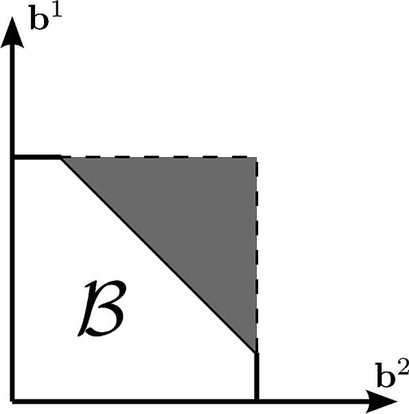
where ⇝ denotes a relaxation and ≡ shows equivalence, ||.||₁ is the ${\ell }_1\text{-norm}$ of a vector which is a convex relaxation of its ${\ell }_0\text{-norm}$ and ≤ is an element-wise inequality constraint. Geometrically, each basis vector, b_j, dwells in the intersection of the ${\ell }_1\text{-norm}$ ball of radius λ with unit ${\ell }_{\infty }\text{-norm}$ ball (box) in the positive orthant, which is shown graphically in Fig.3 for $\mathbf{b}\in {\mathbb{R}}^3$ for sake of illustration. We call the feasible set the Boxed-Sparsity set, in contrast to a feasible set to be defined subsequently.

Fig. 3.

Graphical representation of Boxed-Sparsity for ${\mathbb{R}}^3$, which is the intersection of ${\ell }_{\infty }$ and ${\ell }_1$ norm balls in the positive orthant. The blue dots are vertices of the feasible set.

Group-Sparsity

Another interesting prior on B arises when a partition is available and needs to be taken into account. We assume a common coordinate system by warping all images to a template and an image partitioning (image segmentation) is available for the template image (e.g., an anatomical parcellation in a template space). It is possible to consider sparsity constraint/regularization on the group-level rather than voxel level which promotes that a few groups (e.g., brain structures) are involved in group difference rather than a few voxels. In order to encourage this property, we can enforce an ${\ell }_1\text{-norm}$ on groups instead of voxels. Before defining the idea precisely, we need a few definitions. Assuming $\mathcal{G}$ is a segmentation of an image into sets (g_i's), we can define two group-norms as follows (the idea is graphically shown in Fig.4):

$$\begin{array}{cc}\hfill & {\Vert \mathbf{b}\Vert }_{1,2}:=\sum _{g\in \mathcal{G}}{\rho }_g{\Vert {\mathbf{b}}_{\mid g}\Vert }_2\hfill \\ \hfill & {\Vert \mathbf{b}\Vert }_{\infty ,2}:=\underset{g\in \mathcal{G}}{\text{max}}\left\{{\rho }_g{\Vert {\mathbf{b}}_{\mid g}\Vert }_2\right\}\hfill \end{array}$$ (8)

where b_|g is a D-dimensional vector such that its voxels not belonging to the group g are set to zero, ρ_g is a positive constant that in this paper compensates for a group-size, namely ${\rho }_g=\frac{1}{\mid g\mid }$ where |·| is cardinality of a set. Notice that in the definition of ||·||_1,2, the ${\ell }_2\text{-norm}$ is used instead of ${\ell }_2^2$ because the squared norm does not have the sparsifying properties. This kind of regularization is called Group regularization or Mixed-Norm regularization and have received much attention in recent years in machine learning [35], [36].

Fig. 4.

This figure shows an example of a 3 × 3 image (hence $\mathbf{b}\in {\mathbb{R}}^9$) that is segmented into 3 regions $(\mathcal{G}=\{g_1,g_2,g_3\})$. b_|g1 and ||b||_2,1 shown are as examples. 〈·,·〉, mean inner product thus ${\Vert {\mathbf{b}}_{\mid g_1}\Vert }_2=\sqrt{\langle {\mathbf{b}}_{\mid g_1},{\mathbf{b}}_{\mid g_1}\rangle }$.

Given the new norm definitions in Eq.(8), we can define the Group-Sparsity constraint mathematically as follows:

$$\begin{array}{cc}\hfill & {\Vert \mathbf{b}\Vert }_{1,2}\le \lambda \hfill \\ \hfill & \mathbf{b}\ge 0,{\Vert \mathbf{b}\Vert }_{\infty ,2}\le 1\hfill \end{array}$$ (9)

For the rest of the paper, we will refer to ||b||_1,2 subject to the constraints as Group-Sparsity. Observe the correspondence between Boxed- and Group-Sparsity; in Eq.(9) ||·||_1,2 replaced ||·||₁ and ||·||_∞,2 exchanged for ||·||_∞.

E. Optimization

Given the generative term (Eq.(4)), the discriminative term (Eq.(6)), and the regularization on $\mathbf{w}\left({\Vert \mathbf{w}\Vert }_2^2\right)$, on C(C≥0), and B (Eq.(7) or Eq.(9)), we form an optimization problem as follows:

$$\begin{array}{cc}\hfill \underset{\mathbf{w},\mathbf{B},\mathbf{C}}{\text{min}}{\lambda }_1\mathcal{D}(\mathbf{X};\mathbf{B},\mathbf{C})+& {\lambda }_2\ell (\mathbf{y};\mathbf{X},\mathbf{B},\mathbf{w})+{\Vert \mathbf{w}\Vert }_2^2\hfill \\ \hfill \text{subject to}:& \mathbf{B}\in {\mathcal{B}}_{{\lambda }_3}\hfill \\ \hfill & \mathbf{C}\ge 0\hfill \end{array}$$ (10)

where $\mathcal{D}(\cdot ,\cdot )$ and $\ell (\cdot ;\cdot )$ are given in Eq.(4) and Eq.(6) respectively and ${\mathcal{B}}_{{\lambda }_3}$ is either the Boxed-Sparsity constraint in Eq.(7) or the Group-Sparsity in Eq.(9); λ₁ and λ₂ are relative weights to control importance of the three terms in the objective function; ${\mathcal{B}}_{{\lambda }_3}$ depends on the definition of sparsity, i.e., if the Boxed-Sparsity is chosen λ₃ replaces λ in Eq.(7) or if the Group-Sparsity is selected it substitutes λ in Eq.(8). The ratio $\frac{{\lambda }_2}{{\lambda }_1}$ controls the discriminative power vs. the generative power of the model: the higher the ratio, the more discriminative the model. Throughout the experiments, λ₁ and λ₂ are normalized by the number of samples (i.e., λ₁ λ₂ ∝ $\frac{1}{N}$) and λ₃ is normalized by the dimensionality of the images (i.e., λ₃ ∝ $\frac{1}{D}$). Therefore, we report λ₃ as a percentage value that means $\frac{{\lambda }_3}{D}$ is some percentage of voxels. Note that the objective in Eq.(10), is comprised of three terms; thus, two regularization weights suffice to control the relative ratio of the terms.

Although this optimization is not jointly convex with respect to all variables, it is a block-wise convex program; i.e., if any pair of blocks of variables is fixed, it is a convex optimization problem with respect to the other block. For example, if w and C are fixed, it is a convex optimization problem with respect to B. Therefore, we propose a block-wise optimization scheme shown in Alg.1 that converges to a local minimum. Proof of the convergence to a local minimum follows from the fact that the optimization problem is convex with respect to each block of variables, the objective is lower-bounded and continuous on the domain, and non-differentiable constraints can be added as separable terms to the objective (ref. [37] Prop. 5.1 for more detail).

Algorithm 1.

Block-wise Optimization

Require: Data (X), Labels (y), Regularization (λ's)

initialize B, C, w

k ← 0

repeat

Bk+1 ← argminB J3(B; Ck, wk) (Eq.(13) or (14))

Ck+1 ← argminC J2(C; Bk, wk) (Eq.(12))

wk+1 ← argminw J1(w, Bk, Ck) (Eq.(11))

k ← k + 1

until some convergence criteria satisfied

The optimization is straightforward with respect to two of the blocks (C and w) but challenging with respect to the others (B) that will be discussed in detail subsequently.

1) Optimization w.r.t. w

We start with the most straightforward block. In the k'th iteration, fixing B and C, the optimization should find the global minimum of the following convex function:

$$J_1(\mathbf{w};{\mathbf{B}}^k,{\mathbf{C}}^k)={\lambda }_2\ell (\mathbf{y};\mathbf{X},{\mathbf{B}}^k,\mathbf{w})+{\Vert \mathbf{w}\Vert }_2^2$$ (11)

in which $\ell (\cdot ;\cdot )$ is the loss function defined in Eq.(6). Solving this optimization problem with respect to w is not challenging because it is basically a linear SVM classifier with ${\ell }_2^2$ regularization applied on new features, namely B^Tx_i. Any off-the-shelf solver for a linear SVM can solve Eq.(11) efficiently in a reasonable time because computational complexity of such a solver is bounded by the number of new features (K) and number of samples (N), which are not large in our application. In this paper, we use LIBLINEAR [29] as the solver.

2) Optimization w.r.t. C

Fixing B and w in the k'th iteration, we need to find the global optimum of the following objective with respect to C:

$$\begin{array}{cc}\hfill & J_2(\mathbf{C};{\mathbf{B}}^k,{\mathbf{w}}^k)={\Vert \mathbf{X}-{\mathbf{B}}^k\mathbf{C}\Vert }_F^2\hfill \\ \hfill & \text{subject to}:\mathbf{C}\ge 0\hfill \end{array}$$ (12)

This problem can be easily formulated as a non-negative least squared problem with K × N variables. Given that N is not typically large in medical imaging applications and K is also not large, any off-the-shelf least squared solver can solve this problem. There is an abundant supply of options for nonnegative least squared solvers. We used MOSEK [38] to solve this problem.

3) Optimization w.r.t. B

Fixing C and w in the k'th iteration, a constrained convex programming problem needs to be solved to find optimal B. In the case of Boxed-Sparsity, the following problem needs to be solved:

$$\begin{array}{cc}\hfill J_3(\mathbf{B};{\mathbf{C}}^k,{\mathbf{w}}^k)& ={\lambda }_1{\Vert \mathbf{X}-{\mathbf{BC}}^k\Vert }_F^2+{\lambda }_2\ell (\mathbf{y};\mathbf{X},\mathbf{B};{\mathbf{w}}^k)\hfill \\ \hfill \text{subject to}:& {\Vert {\mathbf{b}}_j\Vert }_1\le {\lambda }_3,1\le j\le K\hfill \\ \hfill & {\Vert {\mathbf{b}}_j\Vert }_{\infty }\le 1,1\le j\le K\hfill \\ \hfill & \mathbf{B}\ge 0\hfill \end{array}$$ (13)

In case of Group-Sparsity, the objective of the optimization problem is as follows:

$$\begin{array}{cc}\hfill \underset{\mathbf{B}}{\text{min}}{J}_3(\mathbf{B};{\mathbf{C}}^k,{\mathbf{w}}^k)& ={\lambda }_1{\Vert \mathbf{X}-{\mathbf{BC}}^k\Vert }_F^2+{\lambda }_2\ell (\mathbf{y};\mathbf{X},\mathbf{B};{\mathbf{w}}^k)\hfill \\ \hfill \text{subject to}:& {\Vert {\mathbf{b}}_j\Vert }_{1,2}\le {\lambda }_3,1\le j\le K\hfill \\ \hfill & {\Vert {\mathbf{b}}_j\Vert }_{\infty ,2}\le 1,1\le j\le K\hfill \\ \hfill & \mathbf{B}\ge 0\hfill \end{array}$$ (14)

where ||b||_∞,2 was defined earlier in Eq.(8).

While Eq.(13) is a constrained quadratic programming, Eq.(14) is a Second Order Cone Programming (SOCP) [34]; nevertheless, solving either case poses a challenge due two reasons: 1) high-dimensionality: for both cases, the number of variables is at least D × K (number of voxels by number of basis vectors) plus [notdef]variables introduced by the non-differentiability of the constraints or objective, and 2) constrained programming subject to a non-smooth feasible set. In general, constrained optimization is more expensive to solve than unconstrained optimization problem.

Projected Gradient (PG) [39] is a first order method that can be used for a constrained problem. However, PG can be slow particularly for non-smooth feasible sets. The newton method is used to accelerate first-order solvers [39]. The Interior Point (IP) method is a variant of the Newton method for a constrained problem [34]. However, the IP method implemented naively fails to solve Eq.(13) or Eq.(14) because IP involves computation and inversion of a Hessian matrix which is prohibitive in term of computation and memory costs. In our experiments, more sophisticated implementations like MOSEK [38] fail to find a point in the feasible set in a reasonable time. Our chosen alternative is use to use Spectral Projected Gradient (SPG) [40] that is a modification of the classical PG method which differs in two essential ways: 1) It uses a non-monotone line search that measures descent with respect to a fixed number of previous iterations instead of just the last iteration. This may lead to a temporary increase in the objective while ensuring overall convergence. 2) It uses spectral step length introduced by Barzilai-Borwein (BB) [41] that gives an initial step length. In the BB approach, the step length (α_t) in t'th iteration is chosen such that α_t^—1 I mimics the Hessian of the objective over the most recent step. Similar approaches have been taken recently by Schmidt et al. [42] and Wright et al. [43] for large-scale non-smooth problems. There are several choices for BB step length [44], in this paper, we choose the following method to compute it [45]:

$$\begin{array}{cc}\hfill & {\mathbf{s}}^k=vec\left({\mathbf{B}}^k\right),{\mathbf{g}}_t=vec(\nabla J_3\left({\mathbf{B}}^k\right))\hfill \\ \hfill & {\mathbf{q}}^k={\mathbf{s}}^k-{\mathbf{s}}^{k-1},{\mathbf{p}}^k={\mathbf{g}}^k-{\mathbf{g}}^{k-1}\hfill \\ \hfill & {\alpha }_{bb}=\frac{{\Vert {\mathbf{q}}^k\Vert }_2}{{\Vert {\mathbf{p}}^k\Vert }_2}\hfill \end{array}$$ (15)

where vec(.) is an operator that reorders elements of a matrix into a vector. We omitted the detail of computation of the gradient of the objective here, for more detail, see Appendix A.

Our proposed algorithm is shown in Alg.(2). It is conceivable that the bottleneck of the algorithm is the projection $\left({\mathcal{P}}_{\mathcal{B}}(\cdot )\right)$ because it should be performed in each iteration. One of the technical contributions of this paper is to suggest an efficient way to perform the projection; see Appendix B for more detail.

Algorithm 2.

Spectral Projected Gradient Solver

Require: Initial point, step-length bounds 0 < αmin < αmax, ν, M

αk ← min{αmax, max{αmin, αbb}}

repeat

$\mathbf{d}\leftarrow {\mathcal{P}}_{\mathcal{B}}({\mathbf{s}}^k-\alpha {\mathbf{g}}^k)-{\mathbf{s}}^k$

$\gamma \leftarrow 1$

M ← maxk-M≤i≤k{J3(si)}

$\mathbf{while}{J}_3({\mathbf{s}}^k+\gamma \mathbf{d})>M+\nu \gamma \langle {\mathbf{g}}^k,\mathbf{d}\rangle \mathbf{do}$

Choose $\gamma \in (0,1)$ with quadratic interpolation [46]

end while

${\mathbf{s}}^k\leftarrow {\mathbf{s}}^k+\gamma \mathbf{d}$

compute BB step-length (αbb) (Eq.(15))

k ← k + 1

until some convergence criteria satisfied

F. An Extension: Semi-Supervised Learning

Semi-supervised learning refers to a class of machine learning techniques that simultaneously use both labeled and unlabeled data for training in settings in which a small amount of labeled data and a large amount of unlabeled data are available. Semi-supervised learning combines elements of unsupervised and supervised learning.

In many medical imaging applications, such situations arise either due to the availability of abundant sample images with no labels, or more importantly due to uncertainty about the labels. For example, recent studies have shown that individuals with Mild Cognitive Impairment (MCI²) tend to progress to Alzheimer's disease (AD) [47]; but not all MCI subjects converge to AD. Recently, several methods have been proposed to address this issue. Sabuncu et al. [48] and Blezek et al. [49] proposed different frameworks for joint image registration and clustering that can exploit unlabeled images. Ribbens et al. [50] suggested a probabilistic method that can incorporate prior clinical information.

In case of semi-supervised learning in our method, some subjects have certain labels (denoted by X_L) and some subjects do not have labels (denoted by X_U). In other words, the data matrix (X) can be partitioned into two sub-matrices, namely X = [X_L X_U]. Our generative-discriminative framework can easily handle such cases. Recall the objective function of the optimization problem in Eq.(10); it was decomposed into three terms: generative term $\left(\mathcal{D}(\cdot ;\cdot )\right)$, discriminative term $\left(\ell (\cdot ;\cdot )\right)$, and regularization term (recall that the constraint can be written as regularization). X_L contributes in both generative and discriminative terms while X_U only contributes in the generative term, namely:

$$\begin{array}{cc}\hfill & ϴ=\{\mathbf{B},\mathbf{C},\mathbf{w}\}\hfill \\ \hfill & \mathcal{J}\left(ϴ\right)=\mathcal{D}(\left[{\mathbf{X}}_L{\mathbf{X}}_U\right];ϴ)+\ell (\mathbf{y};{\mathbf{X}}_L;ϴ)+\mathcal{R}\left(ϴ\right)\hfill \end{array}$$ (16)

in which Θ is introduced to simplify the notation by grouping all parameters into Θ, $\mathcal{J}(\cdot )$ denotes the objective function, $\mathcal{R}(\cdot )$ stands for the regularization terms. Eq.(16) shows that unlabeled samples are not penalized in the discriminative term (the second term) because the true labels are not available for them. This setting will be investigated in Section III.

G. On Selection of the Regularization Parameters

To set values of the parameters (i.e., λ's and r), two strategies are available: first, to embed searching for the best parameters as a part of the training of the algorithm. This strategy is chosen to show the results in this paper; second, to set values of the parameters to pre-defined values which are presumed to perform well. Ideally, the first option is preferred because it potentially yields better performance than setting parameters to pre-defined values, however, the large optimization with respect to (B, C, w) renders searching an expensive task. Although the latter strategy is not investigated in this paper, we will give intuition on how to select parameters to some fixed values.

Parameters of the proposed algorithm are as follows: K number of basis vectors; λ₁, the weight for the generative term; λ₂, the weight for the discriminative term; λ₃, the sparsity ratio for the basis vectors. We propose to choose the parameters in the following order:

1. λ₂: Given Eq.11 and Eq.6, it can be readily derived that $\frac{N}{{\lambda }_2}$ defines the weight for the second term in Eq.11 $\left({\Vert \mathbf{w}\Vert }_2^2\right)$. One suggestion is to run the algorithm for a small-scale dataset for a few iterations and choose λ₂ such that it produces a reasonable classification rate. One can even run the algorithm for a few iterations without the discriminative term and extracts feature (i.e., B^Tx_i) in order to have a sense of an appropriate range for λ₂.

2. K and λ₃: Selection of λ₃ can be inspired by our clinical hypothesis; $\frac{{\lambda }_3}{D}$ approximately sets the non-zero ratio of each basis vector. Depending on our clinical expectations regarding portion of an anatomy (e.g., brain) affected by the disease of interest, we can choose a range for λ₃. However, if sparseness is set to a high value (low λ₃/D), the generative term may not be able to represent the data well because it may not be able to cover the whole domain of images; hence, optimal basis vectors may stay away from the boundaries of the feasible set (where basis vectors achieve 0-1 values) while the model may try to compensate with C to reconstruct the data. In fact, there is a limited budget to reconstruct the data. In order to increase the budget, one can increase the number of basis vectors (K). However, a very large value of K increases the computational cost significantly, so one needs to trade off between excessive sparsity and computational cost. There are also other factors involved in choosing the sparsity ratio that will be discussed in Section III-B.

3. λ₁: Once other parameters are set, we can set a value for λ₁. The ratio $\frac{{\lambda }_2}{{\lambda }_1}$ decides the balance between the generative and the discriminative terms; since λ₂ is already set, one needs to choose the ratio of $\frac{{\lambda }_2}{{\lambda }_1}$. As it will be shown in Section III-A, the algorithm is relatively robust with respect to ratio of λ₁/λ₂ as long as λ₁ is in a reasonable range; hence the value of λ₁ should be chosen such that the first and second terms in Eq.13 have similar magnitude.

III. Experiments

In this section, we conduct several experiments with the proposed method on various data sets and different settings. In the first set of experiments, we will investigate the effect of generative-discriminative trade-off on generalization power of features used for classification. We will also explore the sparsity effect with both definitions of sparsity. The methods will also be compared to other established methods in the literature. We also briefly examine the potentials of the proposed method for semi-supervised learning with both definitions of sparsity for medical imaging datasets. At the end, we investigate effect of the parameter selection on the accuracy rates on datasets that are held out from previous experiments.

A. Generative vs. Discriminative trade-off

The images used in this experiment are structural MR brain images (T1 image) obtained from Alzheimer's Disease Neuroimaging Initiative (ADNI³). 63 normal control (NC) individuals and 54 AD patients were pre-processed via the same pre-processing pipeline. The pre-processing pipeline is designed according to previously validated and published techniques by Goldszal et al. [28]. It includes the following steps: 1) alignment of images to the AC-PC plane; 2) removal of extra-cranial material (skull-stripping); 3) tissue segmentation into gray matter (GM), white matter (WM), and cerebral fluid (CSF), using a brain tissue segmentation method proposed in Pham et al. [51]; 4) non-rigid image warping using the method proposed by Shen et al. [52] to a standardized coordinate system, a brain atlas (template) that was aligned with MNI coordinate space [53]; 5) formation of regional volumetric maps, named RAVENS maps (see [28] and [2]), using tissue-preserving image warping [28]. RAVENS maps quantify the regional distribution of a GM, WM, and CSF, since one RAVENS map is formed for each tissue type. A RAVENS map quantifies an expansion (or contraction) of the tissue modeled by a transformation that warps the image from the original space to the template space. Consequently, voxel values of a RAVENS map in a template space are directly proportional to the volume of the respective structures in the original brain scan. Although this map can be formed for CSF, WM, and GM, we only used maps corresponding to the GM tissue type. An example of GM, WM, and ventricle RAVENS map is shown in Fig.5.

Fig. 5.

Examples of RAVENS maps for the tissue types created from the transformation (ϕ) that warp the template (top, left) to the subject (top, right). The image shows the RAVEN maps for the tree tissue type: Gray Matter (GM, bottom left), White Matter (WM, bottom middle), and Cerebral Spinal Fluid (CSF, bottom right).

In order to investigate the effect of the hybrid generative-discriminative model, we modified the λ₂/λ₁ ratio for various numbers of basis vectors (K). In this experiment, Boxed-Sparsity was used as the sparsity regularization and λ₃ was set to 20% (i.e., λ₃/D = 1/5). The number of basis vectors (K) was chosen from set of {5, 10, 15, 20, 30, 40, 50} to examine robustness of the algorithm to different numbers of basis vectors. As mentioned earlier in the methods section, the proposed algorithm can be viewed as a dimensionality reduction from an original large dimension (D) to smaller but more discriminative and representative dimensions (K); hence so-called projection B^Tx can be viewed as feature extraction. While the original dimension may be too large to apply a non-linear classifier on, we can simply apply a classifier (in this experiment Logistic Model Trees [54] ⁴) on the extracted features (K-dimensional instead of D-dimensional) to boost the performance. For each setting, i.e., a particular ratio of λ₂/λ₁ and number of basis vectors (K), data was split into 10-folds; training including learning (B, C, w) and training a classifier on the extracted features (B^Tx_i), was conducted on 9-fold and the test was carried on the remaining fold. This process was repeated 10 times to compute an average classification accuracy; hence, each point in Fig.7 is the 10-fold cross-validation accuracy. Results are shown in Fig.7. In order to avoid occlusion of the Fig.7a, error-bars (i.e., standard deviations of the accuracy rates) are added as a separate figure (Fig.7b).

Fig. 7.

Average classification rates in 10-fold cross-validation for various ratios of $\frac{{\lambda }_2}{{\lambda }_1}$ (discriminative vs. generative) for different number of basis vectors; i.e., various K. To avoid occlusion, standard deviations of the accuracy rates are added as a separate figure in (b). The y-axis, σ(C.V. Accuracy), indicates the standard deviations of the accuracy rates. The colors are the same as (a).

In Fig.7, as number of basis vector (K) increases, the accuracy rates also increase but they reach a plateau around K ∈ (20, 40). An excessively discriminative model (yellow and violet corresponding to λ₂/λ₁ = 100 and λ₂/λ₁ = 10 respectively) becomes more unstable as the number of basis vector increases while the blue graph, in which the generative term dominates, is quite stable. Increasing the number of basis vectors further, not only increases computational cost drastically but also degrades generalization of the model because of high dimensionality, since the number of samples is of the same order of magnitude (in this experiment N = 117), so we set the maximum number of basis vectors to 50 which is in the same order magnitude. The best performance is shown by red line (λ₂/λ₁ = 0.1) that maintains a balance between the generative and discriminative terms. This graph shows that having the generative term helps to create more stable classification rates. It also shows that unless the algorithm is pushed too much toward the discriminative side, it is fairly robust with respect to choice of parameters; for example for K = 30, perturbations in classification accuracy rates are about 6% for a reasonable range of λ₂/λ₁ (i.e., around 0.01 and 0.1 for this data). Notice that in this cross validation process, every fold contains few samples (between 11 to 13 samples) and 7%-9% missclassification is about one miss classification per fold.

Fig.6 compares basis vectors learned by the proposed algorithm with those of NMF and SVD. The basis vectors are overlaid on the corresponding anatomical template on various slices of sagittal and coronal cuts. In the cases of the proposed algorithm (Fig.6a and Fig.6b) and NMF (Fig.6c and Fig.6d), voxels of the basis vectors with values less than 0.3 are shown transparent for the sake of a better visualization; in case of SVD, values of voxels can be positive or negative, hence only values around zero are set to transparent. Fig.6a and Fig.6b clearly show Hippocampus and temporal lobe which are associated with memory and have been frequently reported [56], [57] and [58] to undergo significant shrinkage in course of the Alzheimer's disease. Hippocampus is also clearly depicted in the basis vector learned by NMF method (Fig.6c and Fig.6d); however, in the basis vector learned by SVD, almost all areas have nonzero positive and negative values and hence it does not clearly show which areas are important.

Fig. 6.

Three examples of basis vectors with three different methods (λ₃/D = 20%): (a) one of the basis vectors learned by the proposed method on sagittal cuts and; (b) coronal cuts. (c) one of the basis vectors learned by the NMF method on sagittal cuts and, (d) coronal cuts. (e) one of the basis vectors learned by the SVD method on sagittal cuts and, (f) coronal cuts.

B. Sparsity Effect

In the previous section (Sec.III-A), the Boxed-Sparsity was used and the ratio of λ₃/D was set to 20%. Given that a large portion of images are dark background, it is a reasonable value. In this section, we investigate different sparsity types (Boxed-and Group-) for different values of λ₃ while keeping number of the basis vectors to a constant (K = 30) that shows roughly the best performance in Fig.7. Fig.8 shows a basis vector as in Fig.6a and Fig.6b but with stronger sparsity constraint (λ₃/D = 10%) to illustrate sparsity effect. It shows more localized areas than those of Fig.6a and Fig.6b. Decreasing λ₃ which enforces stricter sparsity constraint (say λ₃/D = 0.1%) may not be helpful for better representation because as λ₃ decreases, the algorithm has a limited budget of voxels (i.e., few voxels can be selected) to satisfy the generative term $\left(\mathcal{D}(\cdot ;\cdot )\right)$; therefore it prefers to push values of the voxels away from boundaries (i.e., {0, 1}) to satisfy the generative term. Nevertheless, we changed λ₃/D in range of [0.1..0.6] to examine its effect on the classification accuracy (Fig.9). The experiment elaborated in Section III-A is repeated but for different values of λ₃/D and λ₂/λ₁. The settings of the experiment in term of number of samples and pre-processing is identical with those of the experiments in Section III-A.

Fig. 8.

An example basis vector for a strong sparsity constraint (λ₃/D = 10%) in two orthogonal cuts. Compare it with two examples shown in Fig.6 (λ₃/D = 20%) (a) coronal cuts; (b) sagittal cuts.

Fig. 9.

Investigation of sparsity level on the classification accuracy for the Boxed-Sparsity when: (a) the generative term is dominant; (b) the discriminative term is dominant. Standard deviations of the accuracy rates are added as the bars to the figures.

Fig.9 shows comparison of different ratios of λ₃/D for the Boxed-Sparsity for different rates of λ₂/λ₁. Since two types of behaviors are observed, they are shown in two separate graphs for a sake of illustration. Fig.9a shows cases in which the generative term is dominant or moderate while Fig.9b shows graphs in which the discriminative term is dominant.

In Fig.9a, increasing λ₃ (less sparse) slightly improves level of classification accuracy up to a certain point (λ₃/D ∈ [0.2, 0.4] depending on the ratio $\frac{{\lambda }_2}{{\lambda }_1}$) because it yields better reconstruction. However from that point on, it decreases because it means less regularization on the model. Nevertheless, if the generative term is dominant, the algorithm is relatively robust.

Fig.9b shows similar graph for the cases in which the discriminative term is dominant or has relatively higher weight than those of Fig.9a. In this case, increasing λ₃ (decreasing sparsity) deteriorates the classification accuracy. When the discriminative term is dominant, reducing sparsity can approximately be compared to ${\ell }_1\text{-}\mathrm{SVM}$ with small regularization weight; excessive reduction of the regularization weight in ${\ell }_1\text{-}\mathrm{SVM}$ can worsen generalization of the classifier.

Fig. 10 shows an example of a basis vector when Group-Sparsity is used. The feasible set of the Group-Sparsity is smoother than that of the Boxed-Sparsity (Fig.8); in other words, it has fewer sharp corners than the Boxed-Sparsity one. This encourages solutions that are smooth, i.e., voxel values are likely to be in (0, 1) rather than 0 or 1. Nevertheless such behavior is also affected by ${\ell }_2\text{-norm}$ of the samples (i.e., normalization of samples) that are not discussed in this paper in interest of space.

Fig. 10.

An example of a basis vector for a case in which Group-Sparsity constraint is used. (a) coronal cuts; (b) sagittal cuts.

Fig. 11, depicts the same graphs as Fig.9 but for Group-Sparsity regularization. As in Fig.9, the graphs are divided into two (generative- or discriminative- dominant) sub-graphs for a sake of better illustration. In term of maximum accuracy, the Group-Sparsity is comparable with the Boxed-Sparsity (about 3% improvement) but it is more robust with respect to change of parameters; Fig. 10a shows perturbation is accuracy that is about 5% across different settings. In Fig.11b, the Group-Sparsity shows significantly more robust behavior when the discriminative term is dominant comparing to Fig.9b. Such robustness can be explained by definition of the Group-Sparsity regularization. Due to the non-linear relationship within each group, Group-Sparsity imposes fewer degrees of freedom than those of Boxed-Sparsity, therefore it regularizes the objective further. Fig.11b also shows that a reasonable range for Group-sparsity is around $\frac{{\lambda }_3}{D}\in [0.4,0.7]$ which is different that that of the Boxed-Sparsity; the accuracy rates slightly degrade after this range.

Fig. 11.

Investigation of sparsity level on the classification accuracy for the Group-Sparsity when: (a) the generative term is dominant; (b) the discriminative term is dominant. Standard deviations of the accuracy rates are shown as error bars.

C. Comparison with Other Methods

In this section, we compare performance of the proposed algorithm with other methods but first we need to clarify some points about parameter selection (λ's). The dataset is divided into 20 splits, 18 splits are used to learn (B, C, w) and the testing accuracy on one of the two left-out splits is used to search for the best λ's and finally the classification accuracy is reported on the other left-out split.

Table II compares the accuracy rates between five different methods (two of them are variants of the proposed method) on two dataset. Bx and Grp stand for the proposed for Boxed- and Group-Sparsity constraints respectively. Singular Value Decomposition (SVD) and Non-negative Matrix Factorization were added to the table in order to have baseline comparisons. In order to have a fair comparison, number of basis vectors for NMF, SVD, and both variants of the proposed method are set to the same number which is 30. COMPARE is a method proposed by Fan et al. [14] and has shown to perform well on ADNI dataset [59].

TABLE II.

Comparison of the proposed method with two different constraints Boxed-(Bx) and Group-(Grp) with other methods: Singular Value Decomposition (SVD), Non-negative Matrix Factorization (NMF) and COMPARE [14]. AD vs NC is Alzheimer's disease verse Normal Control from ADNI dataset and Lie vs Truth is β-maps of fMRI study for lie detection. The values inside of the parentheses are the standard deviations of the accuracy rates.

	AD vs NC	Lie vs Truth
Bx	86.6%(±14.3%)	84.1%(±20%)
Grp	89.0%(±13.3%)	N/A
SVD	74.2%(±19.3%)	72.5%(±21%)
NMF	62.1%(±16.3%)	55.0%(±10%)
COMPARE	86.7%(±15.3%)	88.3%(±16.3%)

While features extracted from NMF and SVD methods were fed to the same procedure as the proposed method to find the best classifier, COMPARE has it own routine to find an optimal classifier. AD vs NC dataset is already explained in the Section III-A. Lie vs Truth contains 22 subjects performing a forced-choice deception and their brain activations were acquired using BOLD imaging (fMRI). SPM2 software [60] is used to calculate Parameter Estimate Images (PEIs), i.e., regression coefficients or β, of the HRF regressors for each of the 50 conditions from the least mean square fit of the model to the time series. The 50 conditions include forty-eight regressors modeled “lie” and “truth” events individually while two additional regressors modeled the variant distracter and recurrent distracter conditions.

In the Table II, while the Group-sparsity regularization outperforms COMPARE, the Boxed-sparsity performs almost as well as COMPARE on the AD vs NC dataset. On the Lie vs Truth dataset, COMPARE outperforms our method although the Boxed-sparsity is in a reasonable range of the best performance. The Group-Sparsity result for fMRI dataset is shown as “N/A” because fMRI images which are preprocessed with SPM2 are registered to SPM2 atlas with affine transformation. Therefore, structural brain regions of the atlas do not match well with the corresponding regions on the individual subjects that makes the definition of the groups in the Group-Sparsity inaccurate.

The values reported in the Table II for the AD vs NC dataset are in the same range as the accuracy rates reported in [61]; Nevertheless the conditions of the experiments (including pre-processing, features extraction, samples in the training and testing lists, etc.) are different, which make the results not one-to-one comparable.

D. Semi-Supervised Extension

In this section, we investigate an extension of our method to semi-supervised learning proposed in the Section II-F. In order to examine effectiveness of the proposed method for semi-supervised learning, we performed two sets of experiments. In the first set of experiments, the proposed method is compared with well-established semi-supervised methods on a benchmark data published earlier by Schölkopf et al. [62]: in the second sets of experiments, we apply the method on a real medical images acquired from the ADNI dataset.

Table III compares accuracy rates of the proposed method with those of three well-established semi-supervised learning methods on three datasets of a publicly available benchmark [62]. Although the setting in [62] is not in favor of our method and the proposed method is designed to address semi-supervised learning for medical image data, the results can evaluate soundness of the method in a very general context. Full descriptions of the datasets and pre-processing steps are elaborated in [62] but briefly:

TABLE III.

Comparison of classification error rates on a semi-supervised benchmark [62] between the semi-supervised extension of the proposed method and a few well-established methods. SSL-Bx stands for Boxed-Sparsity constrained for mulation in the semi-supervised setting (Section II-F)

	USPS	Text	BCI
SSL-Bx	21.6	35.5	47.23	(Nlabel = 10)
Linear TSVM	30.66	28.6	50.04
non-Linear TSVM	25.20	31.21	49.15
lapSVM	19.05	37.28	49.25
SSL-Bx	13.1	24.8	29.19	(Nlabel = 100)
Linear TSVM	21.12	22.31	42.67
non-Linear TSVM	9.77	24.52	33.25
lapSVM	4.7	23.86	32.39

•USPS

It is a dataset consisting of 150 images of each of the ten digits randomly drawn from the USPS set of handwritten digits. The digits “2” and “5” were assigned to the class +1, and all the others formed class -1. The images were obscured by application of algorithm 21.1 in [62] to prevent people from exploiting spatial relationship of features in the images [62]; more specifically for this dataset: D = 241 and N = 1500.

Text

This is the 5 comp.* groups from the Newsgroups dataset and the goal is to classify the ibm category versus the rest (by Tong et al. [63]); more specifically for this dataset: D = 11, 960 and N = 1500.

BCI

This dataset originates from research toward the development of a brain computer interface (BCI) (Lal et al. [64]). In each trial, EEG (electroencephalography) was acquired from a single subject from 39 electrodes. An autoregressive model of order 3 was fitted to each of the resulting 39 time series. The trail was represented by the total of 117 = 39 × 3 fitted parameters; more specifically for this dataset: D = 117 and N = 400.

In Table III, in the first four rows, number of label samples (N_label) are set to 10 and in the second four rows, it is set to 100. The Table reports error rates for non/linear Transductive Support Vector Machine (TSVM) [65], Laplacian SVM (lapSVM) [66], which are chosen due to their good performance on the three datasets, in addition to the error rate for the proposed method. Entries of the table for lapSVM and non/linear-TSVM are adopted from [62]. According to [62], hyper-parameters of each of the algorithms are chosen by minimizing the test error, which is not possible in real applications; however, the results of this procedure can be useful to judge the potential of a method. To be comparable, similar procedure was applied to find λ₁/λ₂, λ₃/D and K for our algorithm.

Table III shows that no method consistently outperforms other methods across datasets; however, the results are consistent on each dataset. It shows that although our method outperforms others only on the BCI dataset but it is within a reasonable range of the best performance. This result motivates us to employ semi-supervised extension of our method on a real medical image data.

In medical imaging applications, semi-supervised learning arises either due to availability of abundant of sample images with no labels, or more importantly in case that there is uncertainty about the labels. For example Mild Cognitive Impairment (MCI) is viewed as an intermediate stage between normal aging and dementia. It has diverse range of symptoms but when memory loss is the predominant one, it is considered as a risk factor for the Alzheimer's disease (AD) [47]. Recent studies have shown that individuals with MCI incline to progress to the Alzheimer's disease. Grundman et al. [47] estimated an approximate rate of 10% to 15% per year; nevertheless not all MCI subjects converge to the AD. One interesting question would be to determine which MCI subjects have higher likelihood to become AD subject.

In this experiment 238 structural MRI images of MCI subjects were acquired from the ADNI dataset and used as unlabeled data. All 238 MCI subjects have at least 2 scans cor responding to 24-36 months follow-ups. Among 238 subjects, 99 patients have converted to AD at some point by their third year follow ups (MCI-C) and 139 did not convert after three years MCI-NC). AD and NC subjects explained in the Section III-A were used as labeled data and the MCI subjects (MCIC/MCI-NC) were used an unlabeled data. RAVENS maps of the images were computed by the same pre-processing pipeline as those of AD and NC subjects explained in the Section III-A. Similar to the experiments in the Section III-A, labeled data (AD/NC) is divided to 20 folds; data from 19 folds plus unlabeled data (MCI subjects) is used to learn the basis vectors. One fold out of 20 folds of the labeled data plus the unlabeled data were used for testing. In order to avoid searching for the best parameters, the most frequently selected parameters in the Section III-C were used as the parameters.

To evaluate the performance of the algorithm, accuracy rates on the labeled data (AD/NC) and recall rates on the unlabeled data are reported in Table IV for both regularization types. Since unlabeled data is shared between 20 folds, the recall rates (true positive and true negative rates depending on the class label) are averaged among 20 folds.

TABLE IV.

This table shows application of the algorithm in a semi-supervised setting on the ADNI. The accuracy and recall rates (True-Positive and True-Negative rates) for labeled (AD/NC) and unlabeled data (MCI-C/MCI-NC) are shown in the table. ssl-Bx and ssl-Grp indicate semi-supervised setting of the proposed algorithm with the Boxed-Sparsity and Group-Sparsity constraints respectively.

	Accuracy	Recall
	AD vs NC	MCI-C	MCI-NC
SSL-Bx	87.2%(±14.9%)	79.3%(±6.5%)	44.6%(±5.8%)
SSL-Grp	88.9%(±12.3%)	85.4%(±3.6%)	39.9%(±5.9%)

Table IV shows the results for the semi-supervised learning, SSL-Bx/Grp represent semi-supervised learning for the Boxed- and Group-Sparsity constraints respectively. The classification accuracy rates for the labeled data have been improved slightly for the Boxed-Sparsity compared to the Table II meaning that unlabeled data can help improving the classification accuracy for the labeled data. While the recall rates show high values for the MCI-C group, they demonstrate low recall rates for the MCI-NC group. Such low value can partly be described by the fact that the patients in the MCI-NC group have not converted to the AD group yet but they may convert in the future. In addition, the labeled data anchored the classifiers to produce valid results for the AD/NC groups and avoid a case in which all data are assigned to one class. Therefore, Area Under Curve (AUC) of the classifiers should be investigated for further evaluation of the method. For MCI subjects, since a ground truth is not available for MCI-NC subjects, we will investigate this measure in the new experiment.

Observe that for all values reported in Table IV, basis vectors (hence features) extracted in the semi-supervised way but the classifiers are supervised classifier (Logistic Model Trees [54]). One question would be whether a semi-supervised classifier can improve the results. Therefore, we designed an experiment to answer multiple questions: 1) Whether it is helpful to feed the features extracted using semi-supervised basis learning to a semi-supervised classifier instead of a supervised classifier, 2) Whether our semi-supervised basis learning is useful when there are few labeled samples, 3) How the number of labeled samples and different configurations of (semi-)supervised basis learning and (semi-)supervised classifiers affect AUC for MCI subjects.

For computational efficiency, the basis vectors B were learned only from 79 MCI subjects (as unlabeled data), and 20 AD and 20 NC subjects (as labeled data). The labeled subjects were divided into five folds for cross validation (4/5 for training and 1/5 for testing) and the 79 MCI subjects were shared as unlabeled data across folds. In order to investigate the effect of number of labeled data, we performed four basis learning experiments by increasing number of revealed labels from 4 to 32; each fold has 4/5 × (20 + 20) = 32 AD/NC subjects and we revealed labels of AD/NC subjects as: {(2, 2), (4, 4), (8, 8), (16, 16)}. Rest of MCI subjects (i.e., 238—79 = 159) and AD/NC subjects that do not contribute in the basis learning are added to the testing lists for each fold.

After basis learning, features are extracted by projecting all images on the learned basis vectors. These features were fed into a supervised-classifier (Logistic Model Trees [54]) and a semi-supervised classifier (linear Laplacian SVM [67]) to produces labels. To have a reference point for comparison, we also learned the basis without unlabeled data (supervised basis learning). Fig. 12 plots accuracy rates of AD/NC with respect to the number labeled data in different settings. The accuracy rates were computed on the left-out labeled data and the rest of the labeled data that was not introduced during the basis learning or training of the classifier. For brevity, SF in Fig. 12 indicates Supervised Features, i.e., using only labeled data to learn the basis vectors, and SSF denotes Semi-Supervised Features, i.e., using the labeled and the unlabeled data to learn the basis vectors. The figure shows different scenarios for classification: supervised features fed into a supervised classifier (SF + SC) and a semi-supervised classifier (SF + SSF) and compares them with with semi-supervised features fed into a supervised classifier (SSF + SC) and a semi-supervised classifier (SSF + SSF). Fig.12a and Fig.12b show accuracy rates and AUC for the MCI respectively when the Boxed-sparsity is used for regularization and Fig.12c and Fig.12d represent the same quantifies when the Group-sparsity is applied as the sparsity regularization.

Fig. 12.

The accuracy rates and Area Under Curve (AUC) versus different number of labeled samples for different regularizations. SF and SSF stand for supervised and semi-supervised features respectively i.e., supervised basis learning with or without unlabeled data; SC and SSC denote supervised classifier (Logistic Model Trees [54]) or semi-supervised classifier (linear lapSVM) respectively. (a) The accuracy rates of AD/NC when the Boxed-Sparsity is used as regularization. (b) AUC for MCI-NC/MCI-C subjects when the Boxed-Sparsity is used as regularization. (c) The accuracy rates of AD/NC when the Group-Sparsity is used as regularization. (d) AUC for MCI-NC/MCI-C subjects when the Group-Sparsity is used as regularization.

The results shown in Fig. 12 can be summarized as follows:

• semi-supervised classifier helps: in all scenarios in Fig.12 semi-supervised classifiers (i.e., SF+SSC and SSF+SSC) outperform their corresponding supervised classifiers for both types of regularizations (Boxed-Sparsity: Fig.12a-12b, Group-Sparsity: Fig.12c-12d) and both measures (i.e., accuracy and AUC).

• semi-supervised basis learning helps: in all scenarios semi-supervised features (SSF) which are extracted by basis vectors learned in presence of unlabeled data outperform their corresponding supervised features (SF). Significant difference can be seen when the semi-supervised features are fed into semi-supervised classifier (i.e., SSF+SSC) which achieves the best performance for both measures particularly for the Boxed-Sparsity.

Note that semi-supervised features are more stable in terms of performance even if they are fed into a supervised classifier; for example, compare SF+SC and SSF+SC in Fig.12b and Fig.12d. Also note that AUC measures are computed for MCINC/MCI-C subjects because there is no real ground truth for them; hence AUC might be a better measure to show that the classifiers are not biased toward one of the classes although good performances on the labeled data (i.e., AD vs NC) already show this fact.

E. Sensitivity Analysis of the Parameters

In this section, we perform a few experiments to investigate the effect of parameter selection (λ's) on the classification accuracy rates. In this section, instead of optimizing λ's, we set λ's to the most frequently chosen ones in the Section III-C. The MCI subjects were not involved in the experiments of the Section III-C. In addition, we held out 205 AD and NC subjects (89 AD and 114 NC) from the ADNI dataset. Therefore, optimizing λ's in the Section III-C is oblivious with respect to the samples used in this section. In addition to the AD versus NC classification, we have included classification between converter and non-converter MCI subjects to the Table V which is known to be a difficult classification problem [61]. In fact, this experiment shows conservative results for the proposed methods.

TABLE V.

Comparison of the proposed method with two different constraints the Boxed-(Bx) and Group-(Grp) Sparsity with other methods: Singular Value Decomposition (SVD), Non-negative Matrix Factorization (NMF) and COMPARE [14]. AD vs NC is Alzheimer's disease verse Normal Control from ADNI dataset and converter versus non-converter MCI subjects (MCI–C vs MCI–NC). The values inside of the parenthesis are the standard deviations of the accuracy rates.

	AD vs NC	MCI–C vs MCI–NC
Bx	84.2%(±8.3%)	60.7%(±9.4%)
Grp	83.7%(±8.6%)	61.5%(±8.3%)
SVD	70.9%(±14.1%)	57.3%(±2.9%)
NMF	71.8%(±14.7%)	53.5%(±7.8%)
COMPARE	82.2%(±7.4%)	59.4%(±10.5%)

As the Table V shows, the proposed method outperforms other methods on both datasets. The classification rates are relatively low on the MCI-C vs MCI-NC dataset as reported in the literature [61] yet the proposed method shows slightly better performance comparing to other methods in the Table. This experiment shows that as long as the datasets are similar, one can reduce the computational cost of optimizing λ's by removing the extra nested loop for parameter selection (i.e., searching for the best λ's inside of training sets) without significant degradation in the performance of the classifiers.

IV. Discussion and Conclusion

The experiments in this paper show that the algorithm is robust with respect to choice of parameters as long as they are chosen within a reasonable range. It also shows that the generative term is helpful; indeed we have observed in our experiments that in the process of searching for the best λ's, those settings biased toward the generative terms are selected quite frequently. The experiments shows that discriminative term is also essential because in its absence, the formulation becomes more or less similar to NMF [23] formulation which is shown to underperform in Table II. Nevertheless, for very large sample size experiments finding optimal parameters might be computationally expensive. Therefore, in Section II-G, we analyzed the role of each parameter in well-possessedness of the objective function and introduced an intuitive sequence to pick λ's within a reasonable range. In addition, we empirically showed in the Section III-E that as long as datasets are similar one can avoid parameter selection without significant degradation in the accuracy rate.

In Section III-C, we also compared the proposed method with PCA and NMF as baseline methods and COMPARE [14] as the state-of-the-art algorithm. Both variants of the proposed method outperformed the baseline methods (i.e., NMF and PCA) and performed better or almost as well as COMPARE. The Group-sparsity achieved the best performance in AD vs NC but it was not applicable to Lie vs Truth because we defined the groups for the Group-sparsity based on a segmentation of an atlas and all fMRI subjects are brought to the atlas space using only affine registration; it yields inaccurate brain segmentation for each subject and consequently inaccurate definition for the groups. It is also worth mentioning that COMPARE achieves such level of accuracy using 150-250 features while our algorithm uses only 30 basis vectors (i.e., number of features). There is no clear winner between the Group- and the Box-sparsity.

Combination of the generative and the discriminative terms makes extension to a semi-supervised learning readily accessible. We showed in Section III-D that the features extracted in the semi-supervised way are more stable for classification of the the labeled data than the supervised features in spite of scarce labeled data. Again, there is no clear winner when it comes to comparison between the Box-Sparsity and the Group-Sparsity regularization.

There are still several avenues for improvements and extensions that are left for the future work. For example, the framework can be extend to multi-channel images (i.e., when each subject has multiple modalities). Another open field for future research can address approximate alignment. Groups can be defined approximately by associating probability or membership values of each voxel to groups. Such definition of groups changes the definition of unit-ball of the group-sparsity norm and makes the support of the groups to overlap. Defining overlapping groups imposes a challenge to the optimization problem which needs to be addressed. Projection on the unit-ball of the group sparsity for overlapping groups has been recently studied in [68], [69].

This framework can be easily extended to handle multi-class classification. Other regularization terms that enhance the performance of the semi-supervised basis learning (e.g., Laplacian regularization [66]) can be incorporated into the framework. We currently use random initialization but perhaps a multi-scale strategy improves the convergence rate of the algorithm. A faster algorithm can possibly be achieved if the the basis vectors are parameterize by other basis vectors from possibly an over-complete dictionary; it may lead to a convex formulation for the framework instead of the current non-convex formulation.

In summary, we proposed a novel dimensionality reduction that can extract discriminative yet interpretable features. The proposed framework is a hybrid generative and discriminative model that provides a flexible structure: it can incorporate prior knowledge through regularization terms (two variants are proposed in this paper); it can be readily extended to extract features in a semi-supervised way. We formulated the proposed framework as an optimization problem and proposed a novel projection-based algorithm to solve such large scale non-linear problem efficiently. The method was applied on real data in different scenarios and attained superior or comparable results to the state-of-the-art algorithm; at the same time it delineated areas of the difference in the brain which are in agreement with previous clinical studies.

Appendix A

Computing the Gradient of J₃(·)

The objective function consists of two terms: 1) the generative term $\left(\mathcal{D}(\mathbf{X};\mathbf{BC})\right)$, 2) and the discriminative term $\left(\ell (\mathbf{y};\mathbf{X},\mathbf{w},\mathbf{B})\right)$. Derivative of the generative term with respect to B is:

$${\nabla }_{\mathbf{B}}\mathcal{D}(\cdot ;\cdot )={\phi }^{″}\left(\mathbf{BC}\right)\odot (\mathbf{X}-\mathbf{BC})$$

where φ^″ is the second derivative of φ(·) which is set to φ(x) = ½x² in this paper and ☉ is element-wise matrix multiplication. It is worth mentioning that if ½x² is replaced with other choices of a convex function (e.g. x logx) for φ(·), $\mathcal{D}(\cdot ;\cdot )$ yeilds other options for the divergence term (e.g. KL-divergence) to model other assumptions about noise (e.g. Poisson).

Derivative of the discriminative term with respect to k'th column of B is:

$$\begin{array}{cc}\hfill \ell (\mathbf{y};\mathbf{X},\mathbf{w},\mathbf{B})& =\sum _{i=1}^N{\left(\text{max}(0,1-y_i{\mathbf{w}}^T\left({\mathbf{B}}^T{\mathbf{x}}_i\right))\right)}^2\hfill \\ \hfill & =\sum _{i=1}^l{\left(\text{max}(0,1-y_i\sum _{j=1}^K{w}_j{\mathbf{b}}_j^T{\mathbf{x}}_i)\right)}^2\hfill \end{array}$$

$$\begin{array}{cc}\hfill {\nabla }_{{\mathbf{b}}_k}\ell (\cdot ;\cdot )& =\sum _{i\in \mathcal{I}}^N(1-y_i\sum _{j=1}^K{w}_j{\mathbf{b}}_j^T{\mathbf{x}}_i)(-y_i{w}_k{\mathbf{x}}_i)\hfill \\ \hfill & =\sum _{i\in \mathcal{I}}^N(\sum _{j=1}^K{w}_j{\mathbf{b}}_j^T{\mathbf{x}}_i-y_i)\left(w_k{\mathbf{x}}_i\right)\hfill \end{array}$$

in which $\mathcal{I}\equiv \{i\mid 1-y_i{\mathbf{w}}^T\left({\mathbf{B}}^T{\mathbf{x}}_i\right)>0\}$.

Appendix B

Efficient Projections on the Boxed-Sparsity and Group-Sparsity Balls

Euclidean projection operator on a feasible set can be viewed as an optimization problem:

$$\mathcal{P}\left(\mathbf{u}\right)=\text{arg}\underset{\mathbf{z}}{\text{min}}\frac{1}{2}{\Vert \mathbf{u}-\mathbf{z}\Vert }_2^2\mathrm{s}.\mathrm{t}.\mathbf{z}\in \mathcal{B}$$

For Boxed-Sparsity, the problem is a constrained quadratic programming:

$$\begin{array}{cc}\hfill \underset{\mathbf{z}}{\text{min}}& \frac{1}{2}{\Vert \mathbf{u}-\mathbf{z}\Vert }_2^2\hfill \\ \hfill \text{subject to}:& 0\le \mathbf{z}\le 1\hfill \\ \hfill & 1^T\mathbf{z}\le \lambda \hfill \end{array}$$ (17)

Geometrically, the projection point lies either on the boundary of the box in Fig.13 or inside of the box, on the inside boundary of the shaded area in Fig.13. To determine which one, we can simply project the point on the box:

$${\mathcal{P}}_{\text{box}}\left(\mathbf{u}\right)=\text{min}\{1,{\left[\mathbf{u}\right]}_{+}\}$$

where [u]₊ = max{0, u}.

Fig. 13.

Presentation of a feasible set $\left(\mathcal{B}\right)$ for $\mathbf{b}\in {\mathbb{R}}^2$.

If ${\mathcal{P}}_{\text{box}}\left(\mathbf{u}\right)$ still lies outside of the feasible set, it means that the projection point is on the inside boundary of the shaded area. To find the projection in this case, this problem should be solved:

$$\begin{array}{cc}\hfill \underset{\mathbf{z}}{\text{min}}& \frac{1}{2}{\Vert \mathbf{u}-\mathbf{z}\Vert }_2^2\hfill \\ \hfill \text{subject to}:& 0\le \mathbf{z}\le 1\hfill \\ \hfill & 1^T\mathbf{z}=\lambda \hfill \end{array}$$ (18)

Lagrangian of Eqn.(18) is:

$$\mathcal{L}(\mathbf{z},\zeta ,\theta ,\eta )=\frac{1}{2}{\Vert \mathbf{z}-\mathbf{u}\Vert }_2^2+\theta (\sum _{i=1}^D{z}_i-\lambda )-\langle \zeta ,\mathbf{z}\rangle +\langle \eta ,\mathbf{z}-1\rangle$$ (19)

where $\theta \in \mathbb{R}$ and $\eta ,\zeta \in {\mathbb{R}}_{+}^D$ are Lagrangian multipliers. Differentiating it with respect to z and setting it to zero, yields optimality condition: $\frac{\partial \mathcal{L}}{\partial z_i}=z_i-u_i+\theta -{\zeta }_i+{\eta }_i=0$. By complementary slackness of KKT condition, we know whenever z_i > 0 theζ = 0 and whenever z_i < 1 then η_i = 0. Hence, if 0 < z_i < 1 then:

$$z_i=u_i-\theta +{\zeta }_i-{\eta }_i=u_i-\theta$$ (20)

In order to determine optimal solution, z_i, we need to determine θ and indices for which z_i's are zero or one. If indices of ones and zeros of z are given, complementary slackness of KKT condition and the optimality conditions of Eqn.(18) suffices to find optimal θ:

$$\theta =\frac{1}{\mid \mathcal{I}\mid }(\sum _{i:z_i=1}1+\sum _{i\in \mathcal{I}}{z}_i-\lambda )$$ (21)

where $\mathcal{I}=\{i\in \left[n\right]:0<z_i<1\}$ and $\mid \mathcal{I}\mid$ is cardinality of this set.

Following lemmas help us to determine the indices ⁵:

Lemma 1: [71] Let z be the optimal solution to the minimization in Eqn.(18). Let s and j be two indices such that u_s > u_j. If z_s = 0 then z_j must be zero as well.

Proof 1: We will propose a similar lemma for the upper bound:

Lemma 2: Let z be the optimal solution to the minimization in Eqn.(18). Let s and j be two indices such that u_s > u_j. If z_j = 1 then z_s must be 1 as well.

Proof 2: The proof is by contradiction, similar to Lemma 1. Assume that z* is optimal solution and there exist indices j and s such that u_j < u_s and $z_j^{\ast }=1$ but $z_s^{\ast }<1$. Now, let us assume that new vector ẑ that is equal to z* except in two indices j and s in which ${\widehat{z}}_s=z_j^{\ast }$ and ${\widehat{z}}_j=z_s^{\ast }$. It can be readily checked that ẑ is also feasible. The difference in objective value for new vector is:

$$\begin{array}{cc}\hfill {\Vert \mathbf{u}-{\mathbf{z}}^{\ast }\Vert }_2^2-{\Vert \mathbf{u}-\widehat{\mathbf{z}}\Vert }_2^2& ={(u_j-z_j^{\ast })}^2+{(u_s-z_s^{\ast })}^2-{(u_j-{\widehat{z}}_j)}^2-{(u_s-{\widehat{z}}_s)}^2\hfill \\ \hfill & =-2u_j{z}_j^{\ast }-2u_s{z}_s^{\ast }+2u_j{\widehat{z}}_j+2u_s{\widehat{z}}_s\hfill \\ \hfill & =2z_s^{\ast }(u_j-u_s)+2z_j^{\ast }(u_s-u_j)\hfill \\ \hfill & =2(z_j^{\ast }-z_s^{\ast })(u_s-u_j)\ge 0\hfill \end{array}$$

which contradicts with optimality of z*.

Given the lemmas, we can form an optimization problem similar to Eqn.(18). For a fixed θ, we solve the following optimization problem:

$$\begin{array}{cc}\hfill \underset{\mathbf{z}}{\text{min}}& \frac{1}{2}{\Vert (\mathbf{u}-\theta 1)-\mathbf{z}\Vert }_2^2\hfill \\ \hfill \text{subject to}:& 0\le \mathbf{z}\le 1\hfill \end{array}$$ (22)

and then we search over θ such that the solution z satisfies the equality constraint in Eqn.(18). Observe that the term with θ in Eqn.(19) is absorbed into the quadratic term in Eqn.(22). However, Eqn.(22) has a closed form solution:

$${\mathbf{z}}_{\theta }^{\ast }=\text{min}\{1,{[\mathbf{u}-\theta 1]}_{+}\}$$ (23)

Since we do not know the appropriate θ, we need to search for it. So far, optimization problem has simplified from D-dimensional to one dimensional problem. However, the two lemmas help us to find exact θ in finite number of iterations. The idea is to shrink [θ_min, θ_max] with a bisection-type algorithm until number of zeros and ones stay unchanged, then θ can be found exactly with Eqn.(21). The details of the algorithm are shown in Alg.3.

Algorithm 3.

Efficient Projection on Boxed-Sparsity Ball

Require: Input u, λ

z ← min{1, max{0, u}}

if z is infeasible then

θ1 ← 2 maxi zi

θ2 ← mini zi

y1 ← min{1, [u – θ11] +}

y2 ← min{1, [u – θ21] + }

θ ← θ2 + ½(θ2 –θ1)

while True do

z ← min{1, [u – θ1]+}

if 1Tz > λ then

θ2 ← θ

θ ← θ2 + ½(θ2 – θ1)

y2 ← z

else if 1Tz < λ then

θ1 ← θ

θ ← θ2 + ½(θ2 – θ1)

y1 ← z

else

return the z

end if

if numbers of {0,1} of z, y1, and y2 are unchanged

then

$\mathcal{I}\leftarrow \{j\in \left[D\right]:0<z_j<1\}$

$\theta \leftarrow \frac{1}{\mid \mathcal{I}\mid }({\sum }_{z=1}1+{\sum }_{i\in \mathcal{I}}{z}_i-\lambda )$

z ← min{1, [u – θ1] +}

return z

end if

end while

else

return z

end if

Given Alg.(3), efficient projection on a Group-Sparsity ball is very simple because it uses Alg.(3) as a submodule. An algorithm for efficient projection on a Group-Sparsity ball is shown in Alg.(4). In this case, the following optimization problem should be solved:

$$\begin{array}{cc}\hfill & \underset{\mathbf{z}}{\text{min}}\frac{1}{2}{\Vert \mathbf{u}-\mathbf{z}\Vert }_2^2\hfill \\ \hfill & \text{subject to}:1^T\mathbf{t}\le \lambda \hfill \\ \hfill & {\rho }_g{\Vert {\mathbf{z}}_{\mid g}\Vert }_2\le t_g,{\forall }_g\in \mathcal{G}\hfill \\ \hfill & \mathbf{z}\ge 0,\mathbf{t}\ge 1\hfill \end{array}$$ (24)

where t is a positive $\mid \mathcal{G}\mid \text{-dimensional}$ vector and t_g is g'th element of that and ρ_g is a constant. Eqn.(24) ia a Second Order Cone Programming (SOCP) and may look significantly different from Eqn.(17) but a careful inspection reveals that an efficient algorithm to solve Eqn.(17) (Alg.(3)) can help us to solve Eqn.(24) by defining:

$$\mathbf{v}\in {\mathbb{R}}^{\mid \mathcal{G}\mid },v_g={\rho }_g{\Vert {\left[{\mathbf{u}}_{\mid g}\right]}_{+}\Vert }_2$$

Algorithm 4.

Efficient Projection on Group-Sparsity Ball

Require: Input u, λ

if ||[u]+||1,2 > λ then

Form vector v as follows: vg = ρg|| [u|g] + ||2

t ← ProjectBoxedSparsity(v, λ) (Alg.(3))

$\mathrm{for}\mathrm{all}g\in \mathcal{G}\mathbf{do}$

${\mathbf{z}}_{\mid g}\leftarrow \frac{z_g}{v_g}{\mathbf{u}}_{\mid g}$

end for

return z

else

return z

end if

The defined v can be provided as input to Alg.(3) to find a projection in ${\mathbb{R}}^{\mid \mathcal{G}\mid }$ space. Given the projected point, simple rescaling yields optimal z. The procedure is explained in Alg.(4).

Recently there have been a few research papers about efficient projection on the group-sparsity ball for arbitrary definition of the groups. Although it has been shown that projection on group-sparsity ball for arbitrary group is possible [68], it is an expensive operation unless some special structures are assumes for the groups [69] (e.g., tree structure).

References

- 1.Teipel SJ, Born C, Ewers M, Bokde ALW, Reiser MF, Mller H-J, Hampel H. Multivariate deformation-based analysis of brain atrophy to predict alzheimer's disease in mild cognitive impairment. Neuroimage. 2007 Oct;38(1):13–24. doi: 10.1016/j.neuroimage.2007.07.008. [DOI] [PubMed] [Google Scholar]
- 2.Davatzikos C, Genc A, Xu D, Resnick SM. Voxel-based morphometry using the ravens maps: methods and validation using simulated longitudinal atrophy. Neuroimage. 2001 Dec;14(6):1361–1369. doi: 10.1006/nimg.2001.0937. [DOI] [PubMed] [Google Scholar]
- 3.Wright IC, McGuire PK, Poline JB, Travere JM, Murray RM, Frith CD, Frackowiak RS, Friston KJ. A voxel-based method for the statistical analysis of gray and white matter density applied to schizophrenia. Neuroimage. 1995 Dec;2(4):244–252. doi: 10.1006/nimg.1995.1032. [DOI] [PubMed] [Google Scholar]
- 4.Ashburner J, Friston KJ. Voxel-based morphometry–the methods. Neuroimage. 2000 Jun;11(6 Pt 1):805–821. doi: 10.1006/nimg.2000.0582. [DOI] [PubMed] [Google Scholar]
- 5.Snook L, Plewes C, Beaulieu C. Voxel based versus region of interest analysis in diffusion tensor imaging of neurodevelopment. Neuroimage. 2007 Jan;34(1):243–252. doi: 10.1016/j.neuroimage.2006.07.021. [DOI] [PubMed] [Google Scholar]
- 6.Friston KJ, Holmes AP, Worsley KJ, Poline JP, Frith CD, Frackowiak RSJ. Statistical parametric maps in functional imaging: A general linear approach. Human Brain Mapping. 1994;2(4):189–210. [Google Scholar]
- 7.Hua X, Leow AD, Lee S, Klunder AD, Toga AW, Lepore N, Chou Y-Y, Brun C, Chiang M-C, Barysheva M, Jack CR, Bernstein MA, Britson PJ, Ward CP, Whitwell JL, Borowski B, Fleisher AS, Fox NC, Boyes RG, Barnes J, Harvey D, Kornak J, Schuff N, Boreta L, Alexander GE, Weiner MW, Thompson PM, Initiative ADN. 3d characterization of brain atrophy in alzheimer's disease and mild cognitive impairment using tensor-based morphometry. Neuroimage. 2008 May;41(1):19–34. doi: 10.1016/j.neuroimage.2008.02.010. [DOI] [PMC free article] [PubMed] [Google Scholar]
- 8.Salmon E, Collette F, Degueldre C, Lemaire C, Franck G. Voxel-based analysis of confounding effects of age and dementia severity on cerebral metabolism in alzheimer's disease. Hum Brain Mapp. 2000 May;10(1):39–48. doi: 10.1002/(SICI)1097-0193(200005)10:1<39::AID-HBM50>3.0.CO;2-B. [DOI] [PMC free article] [PubMed] [Google Scholar]
- 9.Cox DD, Savoy RL. Functional magnetic resonance imaging (fmri) ”brain reading”: detecting and classifying distributed patterns of fmri activity in human visual cortex. Neuroimage. 2003 Jun;19(2 Pt 1):261–270. doi: 10.1016/s1053-8119(03)00049-1. [DOI] [PubMed] [Google Scholar]
- 10.Davatzikos C. Why voxel-based morphometric analysis should be used with great caution when characterizing group differences. Neuroimage. 2004 Sep;23(1):17–20. doi: 10.1016/j.neuroimage.2004.05.010. [DOI] [PubMed] [Google Scholar]
- 11.Batmanghelich N, Taskar B, Davatzikos C. A general and unifying framework for feature construction, in image-based pattern classification. Inf Process Med Imaging. 2009;21:423–434. doi: 10.1007/978-3-642-02498-6_35. [DOI] [PubMed] [Google Scholar]
- 12.Carroll MK, Cecchi GA, Rish I, Garg R, Rao AR. Prediction and interpretation of distributed neural activity with sparse models. Neuroimage. 2009 Jan;44(1):112–122. doi: 10.1016/j.neuroimage.2008.08.020. [DOI] [PubMed] [Google Scholar]
- 13.Cuingnet R, Chupin M, Benali H, Colliot O. Spatial and anatomical regularization of svm for brain image analysis. Proc. Neural Information Processing Systems NIPS 2010. 2010.
- 14.Fan Y, Shen D, Gur RC, Gur RE, Davatzikos C. Compare: classification of morphological patterns using adaptive regional elements. IEEE Trans Med Imaging. 2007 Jan;26(1):93–105. doi: 10.1109/TMI.2006.886812. [DOI] [PubMed] [Google Scholar]
- 15.Yushkevich P, Joshi S, Pizer SM, Csernansky JG, Wang LE. Feature selection for shape-based classification of biological objects. Inf Process Med Imaging. 2003 Jul;18:114–125. doi: 10.1007/978-3-540-45087-0_10. [DOI] [PubMed] [Google Scholar]
- 16.Golland P, Grimson WEL, Shenton ME, Kikinis R. IN IPMI. SpringerVerlag; 2001. Deformation analysis for shape based classification; pp. 517–530. [Google Scholar]
- 17.LaConte S, Strother S, Cherkassky V, Anderson J, Hu X. Support vector machines for temporal classification of block design fmri data. Neuroimage. 2005 Jun;26(2):317–329. doi: 10.1016/j.neuroimage.2005.01.048. [DOI] [PubMed] [Google Scholar]
- 18.Chu C, Ni Y, Tan G, Saunders CJ, Ashburner J. Kernel regression for fmri pattern prediction. Neuroimage. 2010 Mar; doi: 10.1016/j.neuroimage.2010.03.058. [DOI] [PMC free article] [PubMed] [Google Scholar]
- 19.Thomaz CE, Boardman JP, Hill DL, Hajnal JV, Edwards DD, Rutherford MA, Gillies DF, Rueckert D. Using a maximum uncertainty lda-based approach to classify and analyse mr brain images. Medical Image Computing and Computer-Assisted Intervention MICCAI 2004. 2004;3216:291–300. [Google Scholar]
- 20.Bouchard G. ICMLA ’07: Proceedings of the Sixth International Conference on Machine Learning and Applications. IEEE Computer Society; Washington, DC, USA: 2007. Bias-variance trade-off in hybrid generative-discriminative models; pp. 124–129. [Google Scholar]
- 21.Principled Hybrids of Generative and Discriminative Models. Vol. 1. IEEE Computer Society; Washington, DC, USA: Jul, 2006. [Google Scholar]
- 22.Bosch A, Zisserman A, Muoz X. Scene classification using a hybrid generative/discriminative approach. Pattern Analysis and Machine Intelligence, IEEE Transactions on. 2008 Apr;30(4):712–727. doi: 10.1109/TPAMI.2007.70716. [DOI] [PubMed] [Google Scholar]
- 23.Lee DD, Seung HS. Learning the parts of objects by nonnegative matrix factorization. Nature. 1999 Oct;401(6755):788–791. doi: 10.1038/44565. [DOI] [PubMed] [Google Scholar]
- 24.Hoyer PO. Non-negative matrix factorization with sparseness constraints. 2004:1457–1469. [Google Scholar]
- 25.Singh A, Gordon G. A unified view of matrix factorization models. In: Daelemans W, Goethals B, Morik K, editors. Machine Learning and Knowledge Discovery in Databases, ser. Lecture Notes in Computer Science. Vol. 5212. Springer Berlin Heidelberg; Berlin, Heidelberg: 2008. pp. 358–373. ch. 24. [Google Scholar]
- 26.Dhillon IS, Sra S. Generalized nonnegative matrix approximations with bregman divergences. Neural Information Proc. Systems. 2005:283–290. [Google Scholar]
- 27.Hofmann T. Probabilistic latent semantic analysis. Proc. of Uncertainty in Artificial Intelligence. 1999. pp. 289–296.
- 28.Goldszal AF, Davatzikos C, Pham DL, Yan MX, Bryan RN, Resnick SM. An image-processing system for qualitative and quantitative volumetric analysis of brain images. J Comput Assist Tomogr. 1998;22(5):827–837. doi: 10.1097/00004728-199809000-00030. [DOI] [PubMed] [Google Scholar]
- 29.Fan R-E, Chang K-W, Hsieh C-J, Wang X-R, Lin C-J. Liblinear: A library for large linear classification. Journal of Machine Learning Research. 2008 Aug;9:1871–1874. [Google Scholar]
- 30.Burges CJC. A tutorial on support vector machines for pattern recognition. Data Mining and Knowledge Discovery. 1998;2:121–167. [Google Scholar]
- 31.Biggs M, Ghodsi A, Vavasis S. Proceedings of the 25th international conference on Machine learning, ser. ICML ’08. ACM; New York, NY, USA: 2008. Nonnegative matrix factorization via rank-one downdate; pp. 64–71. [Google Scholar]
- 32.Donoho D, Stodden V. When does non-negative matrix factorization give a correct decomposition into parts. 2003.
- 33.Ng AY. ICML ’04: Proceedings of the twenty-first international conference on Machine learning. ACM; New York, NY, USA: 2004. Feature selection, l1 vs. l2 regularization, and rotational invariance; p. 78+. [Google Scholar]
- 34.Boyd S, Vandenberghe L. Convex Optimization. Cambridge University Press; Mar, 2004. [Google Scholar]
- 35.Obozinski G, Taskar B. Multi-task feature selection. Tech. Rep. 2006 [Google Scholar]
- 36.Huang J, Zhang T. The benefit of group sparsity. Mar, 2009.
- 37.Tseng P. Convergence of a block coordinate descent method for nondifferentiable minimization. J. Optim. Theory Appl. 2001;109(3):475–494. [Google Scholar]
- 38.The mosek optimization software.
- 39.Bertsekas DP, Bertsekas DP. Nonlinear Programming. 2nd ed. Athena Scientific; Sep, 1999. [Google Scholar]
- 40.Birgin EG, Martínez JM, Raydan M. Nonmonotone spectral projected gradient methods on convex sets. 4. Vol. 10. Society for Industrial and Applied Mathematics; Philadelphia, PA, USA: 2000. pp. 1196–1211. [Google Scholar]
- 41.Barzilai J, Borwein JM. Two-point step size gradient methods. IMA J Numer Anal. 1988 Jan;8(1):141–148. [Google Scholar]
- 42.Schmidt M, van den Berg E, Friedlander MP, Murphy K. Optimizing costly functions with simple constraints:a limited-memory projected quasi-newton algorithm. 12th International Conference on Artificial Intelligence and Statistics (AISTATS), ser. JMLR: Workshop and Conference Proceedings series, vol. 2009;5:456–463. [Google Scholar]
- 43.Wright SJ, Nowak RD, Figueiredo MAT. Sparse reconstruction by separable approximation. IEEE Transactions on Signal Processing. 2009 Jul;57(7):2479–2493. [Google Scholar]
- 44.Dai Y-H, Hager WW, Schittkowski K, Zhang H. The cyclic barzilai–borwein method for unconstrained optimization. IMA J Numer Anal. 2006 Jul;26(3):604–627. [Google Scholar]
- 45.Varadhan R, Roland C. Simple and globally convergent methods for accelerating the convergence of any em algorithm. Scandinavian Journal of Statistics. 2008;35(2):335–353. [Google Scholar]
- 46.Grippo L, Lampariello F, Lucidi S. A nonmonotone line search technique for newton's method. SIAM Journal on Numerical Analysis. 1986;23(4):707–716. [Google Scholar]
- 47.Grundman M, Petersen RC, Ferris SH, Thomas RG, Aisen PS, Bennett DA, Foster NL, Jack CR, Galasko DR, Doody R, Kaye J, Sano M, Mohs R, Gauthier S, Kim HT, Jin S, Schultz AN, Schafer K, Mulnard R, van Dyck CH, Mintzer J, Zamrini EY, Cahn-Weiner D, Thal LJ, Study ADC. Mild cognitive impairment can be distinguished from alzheimer disease and normal aging for clinical trials. Arch Neurol. 2004 Jan;61(1):59–66. doi: 10.1001/archneur.61.1.59. [DOI] [PubMed] [Google Scholar]
- 48.Sabuncu MR, Balci SK, Shenton ME, Golland P. Image-driven population analysis through mixture modeling. IEEE Trans Med Imaging. 2009 Sep;28(9):1473–1487. doi: 10.1109/TMI.2009.2017942. [DOI] [PMC free article] [PubMed] [Google Scholar]
- 49.Blezek DJ, Miller JV. Atlas stratification. Med Image Anal. 2007 Oct;11(5):443–457. doi: 10.1016/j.media.2007.07.001. [DOI] [PMC free article] [PubMed] [Google Scholar]
- 50.Ribbens A, Maes F, Vandermeulen D, Sueten P. Semisupervised probabilistic clustering of brain mr images including prior clinical information. MCV’10 Proceedings of the 2010 international MICCAI conference on Medical computer vision: recognition techniques and applications in medical imaging. 2010:184–194. [Google Scholar]
- 51.Pham DL, Prince JL. Adaptive fuzzy segmentation of magnetic resonance images. IEEE Trans Med Imaging. 1999 Sep;18(9):737–752. doi: 10.1109/42.802752. [DOI] [PubMed] [Google Scholar]
- 52.Shen D, Davatzikos C. Hammer: hierarchical attribute matching mechanism for elastic registration. IEEE Trans Med Imaging. 2002 Nov;21(11):1421–1439. doi: 10.1109/TMI.2002.803111. [DOI] [PubMed] [Google Scholar]
- 53.Kabani NJ, MacDonald DJ, Holmes CJ, Evans AC. 3d anatomical atlas of the human brain. NeuroImage. 1998;7:S717. [Google Scholar]
- 54.Landwehr N, Hall M, Frank E. Logistic model trees. Machine Learning. 2003:241–252. [Google Scholar]
- 55.Hall M, Frank E, Holmes G, Pfahringer B, Reutemann P, Witten IH. The weka data mining software: An update; sigkdd explorations. 2009;11 [Google Scholar]
- 56.Chetelat G, Desgranges B, Sayette VDL, Viader F, Eustache F, Baron J-C. Mapping gray matter loss with voxel-based morphometry in mild cognitive impairment. Neuroreport. 2002 Oct;13(15):1939–1943. doi: 10.1097/00001756-200210280-00022. [DOI] [PubMed] [Google Scholar]
- 57.Convit A, de Asis J, de Leon MJ, Tarshish CY, Santi SD, Rusinek H. Atrophy of the medial occipitotemporal, inferior, and middle temporal gyri in non-demented elderly predict decline to alzheimer's disease. Neurobiol Aging. 2000;21(1):19–26. doi: 10.1016/s0197-4580(99)00107-4. [DOI] [PubMed] [Google Scholar]
- 58.Kaye JA, Swihart T, Howieson D, Dame A, Moore MM, Karnos T, Camicioli R, Ball M, Oken B, Sexton G. Volume loss of the hippocampus and temporal lobe in healthy elderly persons destined to develop dementia. Neurology. 1997 May;48(5):1297–1304. doi: 10.1212/wnl.48.5.1297. [DOI] [PubMed] [Google Scholar]
- 59.Fan Y, Batmanghelich N, Clark CM, Davatzikos C, Initiative ADN. Spatial patterns of brain atrophy in mci patients, identified via high-dimensional pattern classification, predict subsequent cognitive decline. Neuroimage. 2008 Feb;39(4):1731–1743. doi: 10.1016/j.neuroimage.2007.10.031. [DOI] [PMC free article] [PubMed] [Google Scholar]
- 60.Wellcome department of imaging neuroscience.
- 61.Cuingnet R, Gerardin E, Tessieras J, Auzias G, Lehricy S, Habert M-O, Chupin M, Benali H, Colliot O, Initiative TADN. Automatic classification of patients with alzheimer's disease from structural mri: A comparison of ten methods using the adni database. Neuroimage. 2010 Jun; doi: 10.1016/j.neuroimage.2010.06.013. [DOI] [PubMed] [Google Scholar]
- 62.Chapelle O, Schölkopf B, Zien A, editors. Semi-Supervised Learning. MIT Press; Cambridge, MA: 2006. [Google Scholar]
- 63.Tong S, Koller D. Restricted bayes optimal classifiers. Proceedings of the 17th National Conference on Artificial Intelligence (AAAI) 2000:658–664. [Google Scholar]
- 64.Lal TN, Schrder M, Hinterberger T, Weston J, Bogdan M, Birbaumer N, Schlkopf B. Support vector channel selection in bci. IEEE Trans Biomed Eng. 2004 Jun;51(6):1003–1010. doi: 10.1109/TBME.2004.827827. [DOI] [PubMed] [Google Scholar]
- 65.Joachims T. Transductive learning via spectral graph partitioning. ICML. 2003:290–297. [Google Scholar]
- 66.Sindhwani V, Niyogi P. Beyond the point cloud: from transductive to semi-supervised learning. ICML. 2005:824–831. [Google Scholar]
- 67.Belkin, Mikhail, Niyogi, Partha, Sindhwani, Vikas Manifold Regularization: A Geometric Framework for Learning from Labeled and Unlabeled Examples. Journal of Machine Learning Research. 2006 Nov;7:2399–2434. [Google Scholar]
- 68.Jacob L, Obozinski G, Vert J-P. Group lasso with overlap and graph lasso. Proc. of the 26th Annual International Conference on Machine Learning. 2009:433–440. [Google Scholar]
- 69.Kim S, Xing EP. Tree-guided group lasso for multi-task regression with structured sparsity. Proceedings of the 27th International Conference on Machine Learning (ICML) 2010.
- 70.Duchi J, Singer Y. Efficient online and batch learning using forward backward splitting. Journal of Machine Learning Research. 2009 Dec;10:2899–2934. [Google Scholar]
- 71.Shalev-Shwartz S, Singer Y, Bennett P, Parrado-hernández E. Efficient learning of label ranking by soft projections onto polyhedra. Journal of Machine Learning Research. 2006;7 [Google Scholar]