

Abstract
We have formulated a mathematical model for the rat afferent arteriole (AA). Our model consists of a series of arteriolar smooth muscle cells and endothelial cells, each of which represents ion transport, cell membrane potential, and gap junction coupling. Cellular contraction and wall mechanics are also represented for the smooth muscle cells. Blood flow through the AA lumen is described by Poiseuille flow. The AA model's representation of the myogenic response is based on the hypothesis that changes in hydrostatic pressure induce changes in the activity of nonselective cation channels. The resulting changes in membrane potential then affect calcium influx through changes in the activity of the voltage-gated calcium channels, so that vessel diameter decreases with increasing pressure values. With this configuration, the model AA maintains roughly stable renal blood flow within a physiologic range of blood flow pressure. Model simulation of vasoconstriction initiated from local stimulation also agrees well with findings in the experimental literature, notably those of Steinhausen et al. (Steinhausen M, Endlich K, Nobiling R, Rarekh N, Schütt F. J Physiol 505: 493–501, 1997), which indicated that conduction of vasoconstrictive response decays more rapidly in the upstream flow direction than downstream. The model can be incorporated into models of integrated renal hemodynamic regulation.
Keywords: renal microcirculation, smooth muscle mechanics, calcium transport, vasoconstriction
electrical stimulation or micropipette application of appropriate vasoactive substances onto the surface of arterioles induces not only a local vasomotor response but also a conducted vasomotor response that propagates upstream and downstream along the vessel. Conducted vasomotor responses are believed to be important in the coordination of the microsovascular tone.
Steinhausen et al. (37) analyzed the propagation of vasomotor responses, induced by local electrical stimulation, in split hydronephrotic rat kidneys. Their results indicate that the responses decay with increasing distance from the stimulation site and that the decay is significantly faster upstream than downstream. An explanation for the asymmetric decay rates, which was elusive, is a motivation for the present study.
In a previous study (5), we developed a detailed mathematical model of the myogenic response of a small segment of the afferent arteriole (AA) wall, including the endothelium and the surrounding smooth muscle cells. That model was used to examine the response of the AA segment to changes in mean and pulsatile pressure. Simulation results of that model are consistent with the hypothesis that the AA myogenic response plays an important role in protecting the glomerular capillaries against elevated systolic pressures. The goal of this study is to develop a multicell model of the AA by connecting a series of AA smooth muscle cells and endothelial cells via gap junction coupling and to use the model to study the myogenic response of the AA and its response to local electrical stimulation. The AA model is intended to be used as an essential component in models of integrated renal hemodynamic regulation.
MATHEMATICAL MODEL
Multicell AA model.
The model is an extension of our previous AA cell model (5) and represents a segment of an AA of length L (L ∼300 μm), consisting of a series of Ncell = 101 smooth muscle cell models (5), coupled via their gap junctions and via an endothelial cell layer. (An odd number of smooth muscle cell models were represented so that there is a middle cell that can be stimulated to study any asymmetry in the conduction of vasoconstrictive response.) The model AA segment is connected in series to a fixed resistor, denoted Rend. The inflow pressure [P0(t) at x = 0] and the pressure at the end of the fixed resistor Pend (at x = 2L) are assumed to be known a priori. A schematic diagram is shown in Fig. 1. When the inflow pressure P0 is varied or when a vasoconstrictive or vasodilative response is induced, the pressure at the end of the AA segment, which is denoted P(L, t) and which we refer to as the “outflow pressure,” may also vary. We set Pend to 0 mmHg and Rend to equal the time-averaged value of the total resistance of the unstimulated AA with P0 = 100 mmHg, so that when the inflow pressure P0 = 100 mmHg, the outflow pressure P(L) ≈ 50 mmHg.
Fig. 1.
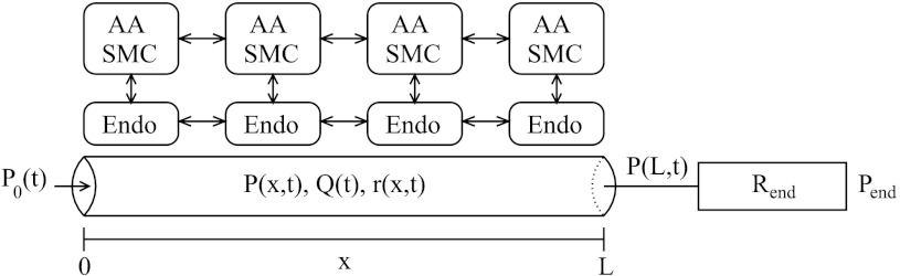
Schematic representation of model afferent arteriole (AA). Hydrodynamic pressure P0(t) drives flow, Q(t), into AA entrance (x = 0) at time t. The model AA is connected to a fixed resistor, Rend, at the end of which pressure is fixed at Pend. Variations in luminal pressure P(x,t) induce myogenic response in AA smooth muscle cells and change luminal radius r(x,t). AA smooth muscle cells (SMC) and endothelial cells (Endo) are coupled by gap junctions.
Each AA smooth muscle cell model incorporates the ionic transports, cell membrane potential, muscle contraction of the AA smooth muscle cells, and the mechanics of a thick-walled cylinder. The model represents the interaction of Ca2+ and K+ fluxes mediated by voltage-gated and voltage-calcium-gated channels, respectively, which gives rise to the periodicity of those transports. This results in a time-periodic cytoplasmic calcium concentration, myosin light chains phosphorylation, and crossbridge formation with the attending muscle stress. The vessel's transmural pressure determines a hoop stress. The resultant hoop, elastic, and muscle stresses determine the rate of change of the vessel's diameter: vasomotion. In addition, the model incorporates the myogenic response mechanism that is based on the hypothesis that the activity of nonselective cation channels is shifted by changes in transmural pressure, such that vessel diameter decreases with increasing pressure and vice versa. A detailed description of the equations for the AA smooth muscle cell model and the model parameters can be found in the appendix and in Ref. 5. Below we describe a few key equations, including those that are modified from the previous model (5).
The rate of change of free cytosolic calcium concentration in the ith smooth muscle cell, denoted Cai, is given by
| (1) |
where α = 1/(zCaβVcellF), zCa = 2 is the valence of the calcium ion, β is the fraction of cell volume occupied by the cytosol, Vcell is the cell volume, F is the Faraday constant, m∞ is the voltage-dependent equilibrium distribution of open calcium channel states, gCa is the maximum whole cell membrane conductance for the calcium current, kCa is the first-order rate constant for cytosolic calcium extrusion, Kd is the ratio of the forward and backward reaction rates of the calcium-buffer system, and BT is the total buffer concentration.
Neighboring AA smooth muscle cell models communicate via their gap junctions. The rate of change of the membrane potential of the i-th cell, vi, is the sum of transmembrane currents:
| (2) |
where C denotes the cell capacitance. The transmembrane leak, potassium, calcium, intersmooth muscle cell gap junction, and smooth muscle-endothelial cell gap junction currents, denoted ILi, IKi, ICai, Igapi, and ISMC-endoi, respectively, are given by ILi = gL (vi − vL), IKi = gK n(vi − vK), ICai = gCam∞ (vi − vCa), Igapi= ggap (vi−1 − 2vi + vi+1), and ISMC-endoi = gSMC-endo (vei − vi), respectively, where gL, gK, and gCa are associated with the respective whole-cell membrane conductances; vL, vK, and vCa denote the respective Nernst reversal potentials; vei denotes the membrane potential of the endothelial cell; and ggap and gSMC-endo are the coupling strengths. Imyoi denotes the current arising from the myogenic response, which is described below.
Myogenic response.
Our model's mechanism for the myogenic response is based on the hypothesis that changes in hydrostatic pressure P induce changes in the activity of nonselective cation channels. The resulting changes in membrane potential then affect calcium influx through changes in the activity of the voltage-gated calcium channels (7). This is represented by the pressure-dependent current Imyoi in Eq. 2 (given in pA), which is described by
| (3) |
here the target current Īmyoi is given by (in pA)
| (4) |
where Pi denotes the transmural pressure (in mmHg), and P*i denotes reference transmural pressure, which is the pressure that the ith cell normally feels. The different rate constants in Eq. 3 corresponding to pressure increase or decrease yield a faster vasoconstriction response compared to vasodilation. Because fluid pressure decreases along the model AA, the AA cells respond to different external environment. Thus we adjust P*i based on the cells' location within the AA, and set P*i to be a linearly decreasing function of its center position (i − ½)Δx, where Δx is the length of one AA subsegment, taken to be 3 μm. More specifically, we set P*i = 100 mmHg − [(i − ½)Δx/L] × 50 mmHg. In the absence of pressure variations, Imyoi = 0.
The AA wall movement is driven by the balance of wall tension, which depends on Pi, and the elastic and contractile forces (5). Because Pi decreases along the AA, wall tension decreases; to ensure force balance, we scale the elastic and contractile forces by a factor ξi that decreases linearly along the AA, from ξi = 1 at x = 0 to ξi = 0.5 at x = L (see Eq. 24).
It has been reported that the AA myogenic mechanism exhibits an asymmetry in its response times for vasoconstriction and vasodilation (24, 25). Loutzenhiser and co-workers (24, 25) observed that the initial delay in the activation of a pressure-dependent vasoconstriction was ∼0.3 s, whereas vasodilation exhibited an initial delay of ∼1 s. To attain that asymmetry, the delay τm in Eq. 4 depends on the rate of change of Pi: τm = 0.3 s for increasing pressure and τm = 1 s for decreasing pressure.
Intercellular communication.
Axial signal propagation along an AA segment takes place through two pathways: gap junctions between neighboring AA smooth muscle cells or conduction through the endothelial cell layer. Communication through AA smooth muscle cell gap junctions is represented by the Igapi term in Eq. 2.
The endothelial cell layer consists of Ncell endothelial cell models; each is connected via gap junctions to an AA smooth muscle cell and to its neighboring endothelial cells. The model represents the membrane potential of the ith endothelial cell, denoted by vei
| (5) |
where Ce denotes the capacitance of the endothelial cell. The first term on the right-side of Eq. 5, gSMC–endo (vi − vei), denotes the gap-junction current between smooth muscle and endothelial cells. The second term, Igap,ei = ggap,e(vei−1 − 2 vei + vei+1), denotes axial gap-junction current.
Axial gap junction communication requires the specification of boundary conditions for the first and last cells (i = 1 and Ncell). In the absence of an electrical stimulation, we assume that the AA is electrically sealed at the two ends, i.e., zero gap-junction currents at the two ends. Thus Igap1 = ggap (−v1 + v2) and IgapNcell = ggap (vNcell−1 − vNcell) . Analogous boundary conditions are applied to the endothelial cells. When a local electrical stimulation is applied to the vessel, a fraction of that current is assumed to exit through the vessel boundaries. The remainder of that current is presumably accounted for by the leak current, so that there is minimal net charge accumulation within the vessel.
Luminal fluid model.
Luminal flow through the model AA is assumed to be at quasi-steady state, and is described by Poiseuille flow
| (6) |
where P is the hydrostatic pressure, μ is the dynamic viscosity of blood, Q is the volumetric flow rate, and r is the luminal radius. As previously noted, the pressure drop across the AA segment and the resistor, given by Pend − P0(t), is assumed to be known a priori. The resistance of the AA segment is given by its luminal radius, which may change due to spontaneous vasomotion, myogenic response, or electrically induced vasomotor response. Given the pressure drop and the total resistance, the volumetric flow Q can be computed as follows:
| (7) |
Once Q is known, we can then update the hydrostatic pressure at each cell.
MODEL RESULTS
Autoregulatory response of the model vessel.
We assessed the model AA's ability to maintain a stable outflow pressure by applying a range of time-independent inflow pressure and computing time-averaged luminal diameters and outflow pressures. Results are shown in Fig. 2. Figure 2A, solid line, shows time-averaged AA diameter profiles for various inflow pressures values, where vasodilation can be seen at low pressure (80 mmHg) and vasoconstriction at higher pressure (120 mmHg). From the outflow pressure values shown in Fig. 2B, solid line, one observes that for inflow pressure between 80 and 180 mmHg, the model AA maintained a somewhat stable outflow pressure that varied between ∼45 and 55 mmHg, where 50 mmHg is the outflow pressure that corresponds to a reference inflow pressure of 100 mmHg. When inflow pressure exceeded 180 mmHg, the model AA failed to adequately compensate, and outflow pressure began to noticeably rise.
Fig. 2.

Space and time-averaged luminal diameter of the AA (A) and outflow pressure (B) as a function of inflow pressure P0 with (solid line) or without (dotted line) myogenic response.
To illustrate the effects of the myogenic response, we simulated the administration of papaverine, which is a smooth muscle relaxant that abolishes autoregulation in the dog kidney (38). We computed outflow pressure while neglecting myogenic response; i.e., we assumed that the activity of the nonselective cation channel is unaffected by changes in transmural pressure. In all simulations, we set Imyoi to 0 for all i′s. In the absence of myogenic response, the model vessel reacts passively to changes in transmural pressure (see Fig. 2, A and B, dotted lines). At higher inflow pressures, the vasodilation reduces vascular resistance, which lowers pressure drop and further increases downstream pressure relative to base case, resulting in a larger vessel diameter downstream (results not shown).
Responses to a step perturbation.
To better understand the characteristic of our AA model, we simulated the time courses of the responses of diameter and pressure to a step increase or decrease in input pressure. Results are shown in Fig. 3.
Fig. 3.

Model responses to a step 20% increase (solid lines) or decrease (dashed line) in AA inflow pressure (A). Changes in AA diameter and outflow pressure are shown in B and C, respectively.
When inflow pressure was increased from 100 to 120 mmHg (Fig. 3A, solid line), the model AA constricted. The time course of the diameter corresponding to the first AA cell is shown in Fig. 3B, solid line. The time courses of the AA diameter at other spatial locations are similar and not shown. The vasoconstrictive response was fully attained after ∼10 s. The outflow pressure initially rose with the inflow pressure, but as the AA constricted, the outflow pressure gradually returned to its reference value of ∼50 mmHg (Fig. 3C, solid line).
When inflow pressure was decreased from 100 to 80 mmHg, the model AA first briefly exhibited a passive constriction and then dilated (Fig. 3B, dashed line). After an initial decline, outflow pressure (Fig. 3C, dashed line) and fluid flow (not shown) returned to their respective references values. Vasodilation was fully attained after ∼20 s.
Responses to sinusoidal oscillations in inflow pressure.
To study the characteristics of the transduction of oscillations in fluid pressure along the AA, we superimposed a sinusoidal perturbation onto the steady-state inflow pressure (x = 0): we applied a pressure of
| (8) |
where P̄0 = 100 mmHg, Pp = 20 mmHg, and f denotes the oscillation frequency. We first studied the model AA's response to a slow sinusoidal perturbation with f = 0.1 Hz. The resulting oscillations in AA luminal diameter and outflow pressure are illustrated in Fig. 4, A2 and A3. The interactions among pressure perturbations, spontaneous oscillations in AA cellular transport and diameter, the asymmetric myogenic response times to pressure increase and decrease, and the coupling among the AA cells through gap junction, endothelial cells, and luminal fluid flow transform the regular oscillations in inflow pressure to highly irregular oscillations in luminal diameter and outflow pressure.
Fig. 4.

Oscillations, as function of time, in AA luminal diameter (A2 and B2) and outflow pressure (A3 and B3) when a sinusoidal perturbation is applied to inflow pressure (A1 and B1). A1–A3: slow oscillations at 0.1 Hz. B1–B3: fast oscillations at 1 Hz. Fast pressure oscillations give rise to a sustained vasoconstrictive response.
Next, we imposed a faster oscillation of f = 1 Hz in the inflow pressure. Note that these pressure oscillations are much faster than the natural frequency of the AA, taken to be the frequency of the spontaneous vasomotion (∼170 mHz). The resulting oscillations in AA luminal diameter and outflow pressure are illustrated in Fig. 4, B2 and B3. Instead of responding to the high-frequency pressure variations passively without attenuation, the model vessel exhibited a sustained vasoconstriction, owing to the cumulative effect of the faster contractile responses (5, 24, 25).
Asymmetric upstream and downstream propagation.
We used the model to analyze the propagation of vasoconstrictive responses, induced by local electrical stimulation, along the AA. That is modeled by adding a depolarization term, Idepoli, to Eq. 2:
| (9) |
We assumed that only the middle AA smooth muscle cell was depolarized. Thus Idepoli = 0 except when i equals the index of the middle AA cell [denoted Nmid = (Ncell + 1)/2], in which case a depolarizing current was applied for t ≥ 20 s:
| (10) |
The value of Idepoli was chosen to achieve a steady-state constricted diameter of ∼10 μm at the stimulation site. To avoid an excessive accumulation of current within the vessel, we assumed that 50% of the depolarizing current exited through the two ends of the model AA. Thus, we set Igap1= ggap (−v1 + v2) − 0.25IdepolNmid and IgapNcell = ggap (vNcell−1 − vNcell) − 0.25IdepolNmid. Because the current leaving the two ends of the AA is the same, any asymmetry in the propagation of the vasomotor response is not caused by boundary conditions.
Figure 5 shows spatial profiles of smooth muscle cell and endothelial cell membrane potentials, luminal pressure, and vascular diameter at three time instances. The profiles labeled “t0” were obtained 0.01 s before the stimulation. At this time, pressure exhibits an approximately linear drop, with vascular diameter and membrane potential oscillating around constant means.
Fig. 5.

Model responses to an electrical stimulation, in membrane potentials v and ve (A), luminal diameter (B), and pressure (C). Profiles are shown for 3 time instances: t0, 0.01 s before stimulation; t1, 0.15 s after simulation; t2, 13.25 s after stimulation.
The profiles labeled “t1” in Fig. 5 show the response of the AA 0.15 s after the electrical stimulation is applied. Note that sufficiently far away from the stimulation site, ve is higher than v, i.e., v lags ve, which indicates that axial propagation of vasoresponse takes place primarily through the gap junctions among the endothelial cells, which are assumed to have much higher conductance than the smooth muscle cell gap junctions. Depolarization raised intracellular Ca2+ concentration of the stimulated cell, and the AA constricted locally. The increase in vascular resistance caused downstream pressure to decrease; in contrast, upstream pressure was not affected. The lower downstream pressure induced a myogenic response there. Note that near the two ends, the vessel was hyperpolarized, i.e., v(t1) < v(t0) near the ends. That transient response is due to the boundary conditions imposed for the smooth muscle cell gap-junction communication, where we assume that a fraction of the stimulating current exits through the vessel ends, thereby transiently and locally hyperpolarizing the vessel.
As the vasomotor response was conducted along the AA, the vessel further constricted and the pressure drop increased. Profiles for membrane potential, luminal pressure, and vascular diameter 13.25 s after the stimulation are shown in Fig. 5, labeled “t2.” The model predicts that while the propagation of the depolarizing current was approximately symmetrical around the stimulation point (see Fig. 5A), the strength of the vasomotor response was stronger downstream (see Fig. 5B). To further illustrate the asymmetry of the vasoconstrictive response, we show the luminal diameters of the upstream-most, middle, and downstream-most cells as functions of time in Fig. 6A. At 30 s after the stimulation, the diameter of the downstream-most cell was ∼80% of the upstream-most one.
Fig. 6.

Propagation of vasoconstrictive response induced by an electrical stimulation. A: responses of selected AA cells as functions of time. B: comparison of model AA diameter profile, given as percentage of maximum response, obtained ∼30 s after stimulation, with exponential fit of measurements by Steinhausen et al. (37).
We also show, in Fig. 6B, the percentage of the maximum response along the AA, obtained ∼30 s after the stimulation. The downstream and upstream decays are approximated by exponential functions with length constants of 340 and 121 μm, respectively. Steinhausen et al. (37) measured similar decay constants of 420 and 150 μm in a vascular tree that comprised mostly of cortical radial artery. The length-to-scale ratio predicted by the model (2.80) matches that of Steinhausen et al.
The above results illustrate that symmetric electrical conduction along the AA (Fig. 5A) transforms into asymmetric mechanical response (Figs. 5B and 6, A and B). That asymmetric decay can be attributed to two factors. The first contributing factor is the shift in the autoregulatory response of a depolarized AA smooth muscle cell. Below we conducted simulations that demonstrate the effect of depolarization on the myogenic-induced vasodilation of an AA smooth muscle cell. Another factor is the differences in the muscle mechanics of the smooth muscle cells, which may have arisen as a result of the adjustments of the smooth muscle cell to their surrounding pressure that, at steady state, decreases approximately linearly in space (see Eq. 24). Assuming that the myogenic response, in terms of the dependence of the nonselective cation channel opening on pressure variations, is the same among the smooth muscle cells, the balance between muscle stresses and wall tension (Eq. 25) differs among different cells except at the steady-state pressure.
To illustrate the above arguments, we simulated the individual myogenic responses of two cells along the AA segment, one at x = L/4 and the other at x = (3/4)L, which we call “upstream cell” and “downstream cell,” respectively. (Note that these two cells were chosen to be equidistant from the midpoint, where the electrical stimulation was applied in the preceding experiment. Since the propagation of the electrical current is approximately symmetric, the two cells' membrane potentials should not differ significantly.) In the following isolated-cell simulations, we prescribed transmural pressure values, simulated only gap-junction current between smooth muscle and endothelial cells, and neglected axial gap junction currents. We computed time-averaged inner diameters of the two cells for a range of pressure perturbations ΔP, given by perturbations from their reference pressure P*, which are 87.5 and 62.5 mmHg, respectively. Results are shown in Fig. 7, the curves labeled “No current.” Both model cells constricted as pressure increased, but constriction was stronger for the upstream cell. Nonetheless, at the pressures that the two cells experienced during the preceding electrical stimulation experiment, which deviated from the upstream and downstream reference pressure values by +2.50 and −25.7 mmHg, respectively (see Fig. 5C), the cell models predicted that the downstream cell was dilated relative to the upstream cell (compare open circles in Fig. 7), a result that is inconsistent with the asymmetric conduction response.
Fig. 7.

Time-averaged AA luminal diameters as a function of perturbation from reference transmural pressure, obtained for an upstream cell (solid lines) and a downstream cell (dashed lines). Simulations were done with a depolarizing current of 0.06 pA and without.
We then repeated the isolated-cell simulations, this time with a depolarizing current of 0.06 pA applied to each cell. That depolarizing current was chosen so that the predicted membrane potentials are similar to their values in the proceeding vasoresponse conduction simulations. The model predicted that, in the presence of the depolarizing current, which induced vasoconstriction in the cells and shifted their autoregulatory curves, the ability of the cells to dilate was impaired. As a result, at lower pressures, the myogenic-induced vasodilation failed to sufficiently compensate for the lower tension force, and the diameter of both cells decreased. The differences in the cells' muscle mechanics also play a role, in that the downstream cells are even less able to dilate at low pressure. Recall that in the preceding electrical stimulation experiment, the upstream and downstream cells experienced fluid pressures that deviated from their reference pressure values by +2.5 and −25.7 mmHg, respectively. At those pressure perturbations, the downstream cell exhibited a diameter that is ∼84% of the upstream cell (compare closed circles in Fig. 7).
To use these results to explain the asymmetric propagation of vasoresponse along the AA vessel, we note that following the application of the depolarizing current, the AA constricted, vascular resistance increased, and downstream pressure decreased. That drop in downstream pressure resulted in two competing effects: a decrease in the tension force arising from transmural pressure, and a vasodilative myogenic response. However, as can be seen in Fig. 7, a depolarized cell cannot effectively dilate, and that impairment is more pronounced for downstream cells. Consequently, the lower tension force dominated downstream, leading to a slower decay of the vasoconstrictive response downstream. In other words, the balance between the two competing effects resulting from the lower downstream pressure-vasoconstriction from the lower tension force and vasodilation from myogenic response shifted in favor of the former when a depolarizing current is applied.
Parameter sensitivity studies.
In the simulations for asymmetric propagation, we set the amount of depolarizing current that exits through the two ends of the vessels, denoted by IBC, to IBC = αBCIdepol51 where αBC = 0.5. To assess the impact of that assumption on model predictions, we conducted a parameter sensitivity study in which we recomputed the conduction length constants for αBC = 0.3, 0.4, 0.6, 0.7. Results are summarized in Table 1. Model predicted that propagation length constants decrease as αBC increases, because as more current was allowed to exit through the ends of the vessel, the extent to which AA was depolarized was reduced (thus, less constriction). This result is consistent with our argument that the asymmetric vasoresponse propagation arises from the shift in the autoregulatory response of a depolarized smooth muscle cell. Nonetheless, in all cases the model predicted a stronger downstream propagation of the vasomotor response, with the downstream-upstream length-scale ratios all fall within 15% of the value (2.80) measured by Steinhausen et al. (37).
Table 1.
Vasoresponse propagation length constants λ for differing boundary conditions
| αBC | Downstream λ, μm | Upstream λ, μm | λ Ratio |
|---|---|---|---|
| Ref. 37 | 420 | 150 | 2.80 |
| 0.3 | 334.95 | 123.58 | 2.71 |
| 0.4 | 383.15 | 131.24 | 2.92 |
| 0.5* | 339.82 | 121.27 | 2.80 |
| 0.6 | 275.97 | 105.65 | 2.61 |
| 0.7 | 211.61 | 87.54 | 2.42 |
The αBC denotes the fraction of depolarizing current that escapes through the ends of the afferent arteriole.
Base case.
The model assumes that the conductance among smooth muscle cells is low compared with that among endothelial cells. To assess model sensitivity to variations in gap-junction coupling, we varied ggap, ggap,e, and gSMC-endo, and we recomputed conduction length constants. Results are shown in Table 2. With stronger coupling, the vasoresponse decayed more slowly along the vessel, in both directions. When ggap,e or gSMC-endo is varied from 80 to 120% of base-case values, the downstream-upstream length-scale ratios λ all fall within 5% of base-case value. Model results are relatively more sensitive to variations in smooth muscle cell coupling. Given the same variations in ggap, λ varies by as much as 13%.
Table 2.
Vasoresponse propagation length constants λ for varying gap-junction coupling constants
| Percentage of base case value, % | Downstream λ, μm | Upstream λ, μm | λ Ratio |
|---|---|---|---|
| Intersmooth muscle cell coupling, ggap | |||
| 120 | 445.36 | 140.58 | 3.17 |
| 110 | 390.36 | 131.37 | 2.97 |
| 100* | 339.82 | 121.27 | 2.80 |
| 90 | 290.31 | 110.01 | 2.64 |
| 80 | 232.25 | 94.40 | 2.46 |
| Interendothelial cell coupling, ggap,e | |||
| 120 | 382.87 | 130.63 | 2.93 |
| 110 | 361.85 | 126.18 | 2.87 |
| 100* | 339.82 | 121.27 | 2.80 |
| 90 | 318.95 | 116.39 | 2.74 |
| 80 | 295.18 | 110.37 | 2.67 |
| Smooth muscle cell-endothelial cell coupling, gSMC-endo | |||
| 120 | 353.94 | 124.15 | 2.85 |
| 110 | 346.21 | 122.72 | 2.82 |
| 100* | 339.82 | 121.27 | 2.80 |
| 90 | 332.72 | 119.80 | 2.78 |
| 80 | 325.68 | 118.29 | 2.75 |
Base case.
DISCUSSION
To study the conduction of vasomotor response along the AA, a phenomenon that is central to the coordination of the responses of individual cells, we have developed a multicell model for the rat AA. The model AA's myogenic response is based on the assumption that changes in hydrostatic pressure induce changes in the activity of nonselective cation channels. The model was used to study the autoregulatory response of the AA, and the mechanism by which vasoconstriction initiated from local sites can spread upstream and downstream along the vessel. Through its myogenic response, the model AA maintained an approximately stable outflow pressure for a range of steady-state inflow pressure from 80 to 180 mmHg. Also, the model predicted pressure-radius relations (Fig. 2A) that are consistent with those obtained in the hydronephrotic rat kidney (24), and with those obtained for isolated rabbit AA, with and without the application of the smooth muscle relaxant papaverine, which abolishes autoregulation (14).
In addition to the above steady-state simulations, we studied the response of the model to oscillating inflow pressure. Simulation results suggest that, owing to the asymmetry in vasoconstriction and vasodilation response times, the AA may be able to sense systolic pressure and respond with a sustained vasoconstriction when systolic pressure is elevated (see Fig. 4, B1 and B2). Similar results were obtained in previous modeling studies (5, 25, 41).
Conduction of vasomotor response.
Krogh et al. (20) once proposed that the mechanism by which a vasodilatory response propagates among the toes of the frog hind limb was provided by the innervation of blood vessels. However, decades of studies in the regulation of microcirculatory blood flow have yielded a better understanding of the ultrastructural organization of the arteriolar networks and an alternative explanation for the conduction of vasomotor response: electrotonic conduction of electrical signaling through the endothelial or smooth muscle cell layer. It has been demonstrated in cheek pouch arterioles that the propagation of vasoconstrictive or vasodilative response is coupled to variations in membrane potential (40, 42), which suggests that the conducted vasomotor response results from the conduction of a electrical signal along the vessel, both upstream and downstream.
Given that the propagation of vasomotor response in arterioles does not appear to depend on flow-mediated changes (e.g., the increased production of NO induced by higher shear stress) or neural transmission, it is generally believed that vasomotor signal is conducted through the endothelial or smooth muscle cell gap junctions. Evidence supporting the role of gap junctions includes the observation that conducted vasomotor responses in hamster cheek pouch are abolished or attenuated with the application of putative gap junction uncouplers (35, 43). Moreover, electron microscopy has demonstrated that neighboring endothelial and smooth muscle cells in renal vasculature (29), thoracic aorta (36), and iridial arterioles (18) are connected by gap junctions, which render these cells electrically and chemically coupled (2, 3, 18, 40, 34, 23, 28, 42, 43). See Ref. 17 for a review on these issues.
When a depolarizing stimulus was applied to one of the AA cells, a local vasoconstrictive response was induced, and that vasomotor response was conducted along the vessel. Vasomotor responses decay with increasing distance from the stimulation site, with a faster decay in the upstream flow direction than downstream, as observed by Steinhausen et al. (37). The mechanisms that account for a directional propagation of vasomotor response were previously not well understood. Steinhausen et al. (37) proposed as potential factors the differences in vessel depths, in electrical conductance of the surrounding tissues, in vascular reactivity between upstream and downstream stimulate sites, in conduction of electrical current, and in transport of biochemical factors in the vascular lumen. Our model results suggest that a depolarizing current reduces the dilation induced by the myogenic response of an AA smooth muscle cell at low pressures, particularly for the downstream cells. That effect shifts the balance between the myogenic response and the reduced tension force among the downstream AA cells in favor of the latter factor, thereby generating a slower decay of the vasoconstrictive response downstream.
The model predicted that the downstream and upstream decays of vasomotor responses are approximated by exponential functions with length constants 340 and 121 μm, respectively. Steinhausen et al. (37) reported decay constants of 420 and 150 μm, respectively. Upstream decay length constants of ∼300–600 μm were measured in renal microvasculature by Wagner et al. (39) for vasoconstriction caused by microapplication of KCl and by Chen et al. (6) for tubuloglomerular feedback (TGF)-initiated vasoconstriction. The upstream decay length constant predicted by our model is smaller than Steinhausen et al. (37) but falls within the range measured in Refs. 6 and 39. The discrepancy in length scales determined by our model and Steinhausen et al. (37) may be attributed to the latter using a vascular tree that comprised mostly of interlobular artery. Nonetheless, the length-to-scale ratios predicted by the model and in the experiments match. Given the preference for propagation downstream, myogenic activation of interlobular artery is likely to be more powerfully transmitted to downstream vascular segments.
Comparison with previous models.
The multicell AA model of the present study is an extension of our previous AA cell model (5), which represents the response of both the smooth muscle cells and the endothelium along a very small segment of the AA, or one single cell. The AA cell model (5) was in turn based on a model for cerebral arterioles in cat that was developed by Gonzalez-Fernandez and Ermentrout (16), with appropriate adjustments in parameters. Consistent with the present study, the AA cell model (5) responded to a high-frequency pressure oscillations with a sustained constriction. The AA model of the present study was constructed by connecting instances of the AA cell model in series, with each cell model coupled to its neighbors through gap junctions, which allows the representation of electrotonic conduction along the AA. A fluid dynamics model was included to relate fluid pressure, fluid flow, and tubular resistance. Also, some of the parameters of the AA cell model were adjusted to depend on the location within the AA because of the decrease in intravascular pressure along the vessel.
Lush and Fray (26) developed a mathematical model of the myogenic control of the AA (hereafter referred to as the L&F model) and used that model to study the steady-state autoregulation of renal blood flow in the dog kidney. Their model computes steady-state renal blood flow assuming a balance of the distensive and constrictive forces acting on the AA. Similar to our model, the AA smooth muscle contraction in the L&F model is assumed to be initiated by pressure-induced changes in calcium permeability, and their model describes the effect of transmural pressure on calcium permeability, intracellular calcium concentration, and contractile activity. Because Lush and Fray focused on steady-state autoregulation, details of the kinetics of the AA ionic transport and muscle mechanics were not represented nor was the asymmetry in the response times of the AA to pressure increase and decrease. Also, individual AA cells are not differentiated in the L&F model. Despite these differences, the L&F model and the present model predicted similar autoregulatory responses (compare Fig. 4 in Ref. 26 and Fig. 2).
Secomb and colleagues (1, 4) developed a model of blood flow regulation. Their model's representations of the active contractile force and resulting muscle mechanics are similar to the L&F model, but the model by Secomb and co-workers represents also metabolic vasoactive and shear stress-dependent responses. Their model was formulated for both large and small arterioles, each with a different set of parameters.
Marsh et al. (27) also adopted the smooth muscle cell model of Gonzalez-Fernandez and Ermentrout (16) to study the interactions between AA myogenic response and TGF. However, as noted in a previous study (5), in Ref. 27 myogenic responses were generated only in response to oscillatory transmural pressure, whereas it has long been observed that changes in mean pressure also induce myogenic responses (24). In contrast, our model exhibits myogenic responses as a function of both pressure and its rate of change. Another difference is that the myogenic model in Ref. (27) represents only two AA segments. Thus each submodel represents a rather long segment along the AA, whereas each of our AA cell submodel roughly corresponds to an AA cell. Both AA segments in Ref. 27 share the same model parameters; in contrast, based on the observation that the AA cells respond different external environments (e.g., intravascular fluid pressure), we adjusted some of the AA cell parameters based on their location within the AA.
Model limitations and future extensions.
Because the model represents a series of AA and endothelial cells, some degree of simplification was necessary to keep computational costs low. Thus the model adopts a phenomenological representation of certain details of the myogenic response. For example, to recapitulate the asymmetric constrictive and dilation kinetics similar to behaviors observed in vitro, the model myogenic mechanism represents asymmetric time delays, based on experimental measurements (24, 25), and assumes a rate-sensitive nonselective cation channels activation. While this model description yields predictions that are consistent with experimental observations (24, 25), potentially important details are neglected, including the possible involvement of ENaC channels in the initiation of the myogenic response, signaling pathways underlying the vascular smooth muscle constriction, or signaling mechanisms that modulate the myogenic response.
Fluid dynamics in the AA is represented as quasi-steady-state Poiseuille flow, which assumes that the flow is laminar and through a long pipe with constant radius. Because the AA walls constrict and dilate, conditions for Poiseuille flow are only approximately satisfied, provided that the amplitude of the vasomotion is sufficiently small, and the time scale of the fluid dynamics is much faster than wall mechanics. A more realistic fluid model would be the Navier-Stokes equations, but the computations required for solving the Navier-Stokes equations are much more time consuming.
Despite its limitations, the present AA model can be used as an essential component in models of integrated renal hemodynamic regulation. By coupling a number of AA models, one can investigate how vasomotor responses propagate among a vascular tree. And using an approach similar to Ref. 27, the AA model could then be combined with a model of glomerular filtration (e.g., Ref. 8) and a model of the TGF mechanism (e.g., Ref. 21) to study the interactions between the myogenic and TGF mechanisms in the context of renal autoregulation.
GRANTS
This research was supported by the National Science Foundation Grant DMS-0715021 and by the National Institute of Diabetes and Digestive and Kidney Diseases Grant DK-053775.
ACKNOWLEDGMENTS
We thank Dr. Leon Moore for bringing to attention the study by Steinhausen et al. (37) and for other helpful discussions.
APPENDIX: MODEL EQUATIONS AND PARAMETERS
This appendix contains model equations that describe the ionic transport and mechanical properties of an AA smooth muscle cell (5), as well as a list of model parameters.
Ion transport and membrane potential.
The smooth muscle cells of the AA can undergo contractions that are determined by the free cytosolic calcium concentration Ca. The sum of Ca and bound buffer CaB gives the total calcium concentration CaT, i.e.,
| (11) |
The free cytosolic calcium and the unbound buffer B combine to yield CaB in a reversible reaction that can be represented by
| (12) |
Because the kinetics of the calcium-buffer system is substantially faster than other relevant membrane transporters, the above reaction is assumed to be at equilibrium. Thus,
| (13) |
By differentiating Eq. 11 with respect to time and using Eq. 13, one obtains
| (14) |
The rate of change of CaT can be described by the following first-order kinetics:
| (15) |
where Vcell is the cell volume; β is the fraction of cell volume occupied the cytosol; F is the Faraday constant; zCa = 2 is the valence of the calcium ion; and kCa is the first-order rate constant for cytosolic calcium extrusion. The m∞ is the equilibrium distribution of open calcium channel states and is described as a function of membrane potential v (15, 22):
| (16) |
where v1 is the voltage at which half of the channels are open, and v2 determines the spread of the distribution.
The opening of potassium channels induces a transmembrane K+ efflux, which polarizes the cell membrane. To represent the K+ flux, we describe the rate of change of the fraction of K+ channel open states, denoted n, by first-order kinetics (30):
| (17) |
where n∞ denotes the equilibrium distribution of open K+ channel states. The rate constant λn is given by
| (18) |
where ϕn determines the rate at which the potassium channels open. This distribution depends on the membrane voltage v and the free cytoplasmic calcium concentration Ca:
| (19) |
where
| (20) |
The potential v3, which determines the voltage at which half of the potassium channels are open, is a function of Ca; v4 and Ca4 are measures of the spread of the distributions of n∞ and v3, respectively.
Myosin phosphorylation.
Oscillations in Ca vary the phosphorylation rate of the 20k-Da myosin light chains (MLC), which are involved in the formation of crossbridges between overlapping myosin and actin filaments. The formation of crossbridges causes smooth muscle contractions. Because the kinetics of that phosphorylation, which is calcium dependent, is much faster than other vasomotion processes considered here, we assume that the fraction of phosphorylated MLC to total MLC, denoted by ψ, is given by (33)
| (21) |
where Cam is a constant. The phosphorylated myosin interacts with actin to form crossbridges and develop stress (19). Let ω denote the fraction of crossbridges formed; then, we describe the net formation of crossbridges by means of the ordinary differential equation given by
| (22) |
Vessel mechanics.
Variations in the number of crossbridges induce variations in a contractile force, which in turn gives rise to variations in AA diameter. To simulate the resulting vasomotion, we consider the blood vessel to be a thick-walled cylinder. The motion of the vessel wall is driven, in part, by the transmural pressure, muscle activity, and wall deformation, which give rise to forces described below. Let ri and ro denote the inner and outer vessel radius, respectively. Let P denote the transmural pressure, and let x denote the average circumferential length, i.e., x = π(ri + ro). The transmural pressure causes the vessel to relax or contract, which then gives rise to a tension force in the angular (θ) direction. That force, which we denote by fP, is given by
| (23) |
where A, the wall cross-sectional area, is given by A = π (ro2 − ri2) (16).
Wall deformation gives rise to additional stresses along the θ-direction of the wall. Let y and u be the circumferential lengths associated with the contractile and series elastic components, respectively. We assume that those stresses consist of the following components: a contractile component of length y, in series with an elastic component of length u; these two components are in parallel with an elastic component of length x = y + u (recall that x is the average circumference). We consider the resulting hoop forces on a surface S, which is bounded by the inner and outer radii of the vessel; S is assumed to be perpendicular to the angular (θ) direction, and to have unit length along the axial direction. Then, given the stresses σx, σy, and σu (see below), the hoop forces on S of the ith AA smooth muscle cell are:
| (24) |
where we and wm are weights representing the contribution by the elastic and muscular components of the hoop forces, and ξi decreases linearly along the AA. The rate of change of the parallel elastic component's length is given by
| (25) |
where τ is a pseudo-time constant associated with the wall internal friction.
For a given number of crossbridges, the velocity of the contractile component (y) is assumed to depend on the balance between the muscle load experienced by the contractile component, given by the elastic stress σu and the contractile stress σy. For σu ≤ σy, the velocity is also proportional to phosphorylation level (9, 10, 32). Thus, following Ref. 16, we have
| (26) |
for σu > σy, the contractile component lengthens:
| (27) |
To approximate experimental measurements (10, 11, 12, 13, 31), the hoop stresses associated with the parallel elastic, contractile, and series elastic components, denoted by σx, σy, and σu, respectively, are given in Ref. 16 by
| (28) |
| (29) |
| (30) |
where σy0 is the reference stress that depends on the fraction of crossbridges formed, ω:
| (31) |
On the right-hand side of Eq. 28, the first term represents the stiff collagen fibers that come into play for large expansions; the second term represents the compliant elastin fibers that play a role in smaller deformations; the third term represents the large stiffness that arises when the vessel radius is substantially reduced; and the fourth term serves to fit σx to experimental data (31).
Parameters.
A large number of parameters are used in this model to describe the AA's geometrical dimensions, membrane transport properties, and muscle mechanical properties. The values of these parameters are given in Tables 3, 4, 5, 6, and 7. Most of the parameters that describe the transport and mechanical properties of the AA smooth muscle cells are taken from Ref. 16 (with some modifications to account for the differences in physical dimensions and in dynamic behaviors between the cerebral arterioles modeled in Ref. 16 and the renal AA) and have previously been reported in Ref. 5.
Table 3.
Afferent arteriole geometric dimensions
| Parameter | Value | Unit |
|---|---|---|
| A | 1.38 × 10⁻⁶ | cm2 |
| L | 303.00 × 10⁻⁴ | cm |
| Ncell | 101 | dimensionless |
| S | 2.00 × 10⁻⁴ | cm2 |
| Δx | 3.00 × 10⁻⁴ | cm |
Table 4.
Smooth muscle cell electrochemical parameters
| Parameter | Value | Unit |
|---|---|---|
| α | 96.62 × 10¹⁵ | nM/C |
| BT | 105 | nM |
| C | 6.5 | pF |
| Ca3 | 400 | nM |
| Ca4 | 150 | nM |
| Cam | 277 | nM |
| ϕn | 0.925 | s−1 |
| gL/C | 1.00 | s−1 |
| gK/C | 4.00 | s−1 |
| gCa/C | 2.00 | s−1 |
| ggap/C | 950 | s−1 |
| gSMC-endo/C | 85 | s−1 |
| Kd | 103 | nM |
| kCa | 190 | s−1 |
| v1 | −22.5 | mV |
| v2 | 25.0 | mV |
| v4 | 14.5 | mV |
| v5 | 8.00 | mV |
| v6 | −15.0 | mV |
| vL | −70.0 | mV |
| vK | −95.0 | mV |
| vCa | 80.0 | mV |
Table 5.
Arteriolar cell parameters
| Parameter | Value | Unit |
|---|---|---|
| gSMC-endo/Ce | 13.60 × 10² | s−1 |
| ggap,e/Ce | 30.40 × 10³ | s−1 |
| C/Ce | 16.0 | dimensionless |
Table 6.
Smooth muscle cell mechanical parameters (I)
| Parameter | Value | Unit |
|---|---|---|
| x0 | 0.0150 | cm |
| x1 | 1.20 | dimensionless |
| x2 | 0.130 | dimensionless |
| x3 | 2.22 | dimensionless |
| x4 | 0.712 | dimensionless |
| x5 | 0.800 | dimensionless |
| x6 | 0.0100 | dimensionless |
| x7 | 0.139 | dimensionless |
| x8 | 0.890 | dimensionless |
| x9 | 9.05 × 10⁻³ | dimensionless |
| u1 | 41.8 | dimensionless |
| u2 | 4.74 × 10⁻² | dimensionless |
| u3 | 5.84 × 10⁻² | dimensionless |
| y0 | 0.928 | dimensionless |
| y1 | 0.639 | dimensionless |
| y2 | 0.350 | dimensionless |
| y3 | 0.788 | dimensionless |
| y4 | 0.800 | dimensionless |
Table 7.
Smooth muscle cell mechanical parameters (II)
| Parameter | Value | Unit |
|---|---|---|
| a | 0.281 | dimensionless |
| b | 5.00 | dimensionless |
| c | 0.0300 | s−1 |
| d | 1.30 | dimensionless |
| kψ | 0.250 | s−1 |
| ψm | 0.300 | dimensionless |
| ωref | 0.685 | dimensionless |
| ψref | 0.599 | dimensionless |
| νref | 0.240 | s−1 |
| σy0# | 1.46 × 10⁷ | dyn/cm2 |
| σ0# | 1.69 × 10⁷ | dyn/cm2 |
| τ | 0.500 | dyn·s·cm−1 |
| we | 1/9.00 | dimensionless |
| wm | 0.700 | dimensionless |
REFERENCES
- 1. Arciero JC, Carlson BE, Secomb TW. Theoretical model of metabolic blood flow autoregulation: roles of ATP release by red blood cells and conducted responses. Am J Physiol Heart Circ Physiol 295: H1562–H1571, 2008 [DOI] [PMC free article] [PubMed] [Google Scholar]
- 2. Beny JL. Electrical coupling between smooth muscle cells and endothelial cells in pig coronary arteries. Pflügers Arch 433: 364–367, 1997 [DOI] [PubMed] [Google Scholar]
- 3. Beny JL, Girbi F. Dye and electrical coupling of endothelial cells in situ. Tissue Cell 21: 797–802, 1989 [DOI] [PubMed] [Google Scholar]
- 4. Carlson BE, Arciero JC, Secomb TW. Theoretical model of blood flow autoregulation: roles of myogenic, shear-dependent, and metabolic responses. Am J Physiol Heart Circ Physiol 295: H1572–H1579, 2008 [DOI] [PMC free article] [PubMed] [Google Scholar]
- 5. Chen J, Sgouralis I, Moore LC, Layton HE, Layton AT. A mathematical model of the myogenic response to systolic pressure in the afferent arteriole. Am J Physiol Renal Physiol 300: F669–F681, 2011 [DOI] [PMC free article] [PubMed] [Google Scholar]
- 6. Chen YM, Yip KP, Marsh DJ, Rathlou Holstein NH. Magnitude of TGF-initiated nephron-nephron interaction is increased in SHR. Am J Physiol Renal Fluid Electrolyte Physiol 269: F198–F204, 1995 [DOI] [PubMed] [Google Scholar]
- 7. Davis MJ, Hill MA. Signal mechanisms underlying the vascular myogenic response. Physiol Rev 79: 387–423, 1999 [DOI] [PubMed] [Google Scholar]
- 8. Deen WM, Robertson CR, Brenner BM. A model of glomerular ultrafiltration in the rat. Am J Physiol 223: 1178–1183, 1972 [DOI] [PubMed] [Google Scholar]
- 9. Dillon PF, Askoy MO, Driska SP, Murphy RA. Myosin phosphorylation and the cross-bridge cycle in arterial smooth muscle. Science 211: 495–497, 1981 [DOI] [PubMed] [Google Scholar]
- 10. Dillon PF, Murphy RA. Tonic force maintenance with reduced shortening velocity in arterial smooth muscle. Am J Physiol Cell Physiol 242: C102–C108, 1982 [DOI] [PubMed] [Google Scholar]
- 11. Dobrin PB. Vascular mechanics. In: Handbook of Physiology. The Cardiovascular System. Peripheral Circulation and Organ Blood Flow, edited by Shepperd JT, Abboud FM, Geiger SR. Bethesda, MD: Am Physiol Soc, sect 2, vol III, 1983, p 65–102 [Google Scholar]
- 12. Dobrin PB, Canfield TR. Identification of smooth muscle series elastic component in intact carotid artery. Am J Physiol Heart Circ Physiol 232: H122–H130, 1977 [DOI] [PubMed] [Google Scholar]
- 13. Driska SP, Damon DM, Murphy RA. Estimates of cellular mechanics in arterial smooth muscle. Biophys J 24: 525–540, 1978 [DOI] [PMC free article] [PubMed] [Google Scholar]
- 14. Edwards RM. Segmental effects of norepinephrine and angiotensin II on isolated renal microvessels. Am J Physiol Renal Fluid Electrolyte Physiol 244: F526–F534, 1983 [DOI] [PubMed] [Google Scholar]
- 15. Ehrenstein G, Lecar H. Electrically gated ionic channels in lipid bilayers. Q Rev Biophys 10: 1–34, 1977 [DOI] [PubMed] [Google Scholar]
- 16. Gonzalez-Fernandez JM, Ermentrout B. On the origin and dynamics of the vasomotion of small arteries. Math Biosci 119: 127–167, 1994 [DOI] [PubMed] [Google Scholar]
- 17. Gustafsson F, Holstein-Rathou NH. Conducted vasomotor responses in arterioles: characteristics, mechanisms and physiological significance. Acta Physiol Scand 167: 11–21, 1999 [DOI] [PubMed] [Google Scholar]
- 18. Hirst GD, Edwards FR, Gould DJ, Sandow SL, Hill CE. Electrical properties of iridial arterioles of the rat. Am J Physiol Heart Circ Physiol 273: H2465–H2472, 1997 [DOI] [PubMed] [Google Scholar]
- 19. Kamm KE, Stull JT. The function of myosin and myosin light chain kinase phosphorylation in smooth muscle. Annu Rev Pharmacol Toxicol 25: 593–620, 1985 [DOI] [PubMed] [Google Scholar]
- 20. Krogh A, Harrop GA, Brandt-Rehberg P. Studies on the physiology of capillaries. III. The innervation of the blood vessels in the hind legs of the frog. J Physiol 56: 179–189, 1922 [DOI] [PMC free article] [PubMed] [Google Scholar]
- 21. Layton AT. Feedback-mediated dynamics in a model of a compliant thick ascending limb. Math Biosci 228: 185–194, 2010 [DOI] [PMC free article] [PubMed] [Google Scholar]
- 22. Lecar H, Ehrenstein G, Latorre R. Mechanism for channel gating in excitable bilayers. Ann NY Acad Sci 264: 304–313, 1975 [DOI] [PubMed] [Google Scholar]
- 23. Little TL, Xia J, Duling BR. Dye tracers define differential endothelial and smooth muscle coupling patterns within the arteriolar wall. Circ Res 76: 498–504, 1995 [DOI] [PubMed] [Google Scholar]
- 24. Loutzenhiser R, Bidani A, Chilton L. Renal myogenic response: kinetic attributes and physiologic role. Circ Res 90: 1316–1324, 2002 [DOI] [PubMed] [Google Scholar]
- 25. Loutzenhiser R, Bidani A, Wang X. Systolic pressure and the myogenic response of the renal afferent arteriole. Acta Physiol Scand 181: 404–413, 2004 [DOI] [PubMed] [Google Scholar]
- 26. Lush DJ, Fray JCS. Steady-state autoregulation of renal blood flow: a myogenic model. Am J Physiol Regul Integr Comp Physiol 247: R89–R99, 1984 [DOI] [PubMed] [Google Scholar]
- 27. Marsh DJ, Sosnovtseva OV, Chon KH, Holstein-Rathlou N-H. Nonlinear interactions in renal blood flow regulation. Am J Physiol Regul Integr Comp Physiol 288: R1143–R1159, 2005 [DOI] [PubMed] [Google Scholar]
- 28. Mekata F. Current spread in the smooth muscle of the rabbit aorta. J Physiol 242: 143–155, 1974 [DOI] [PMC free article] [PubMed] [Google Scholar]
- 29. Mink D, Schiller A, Kriz W, Taugner R. Interendothelial junctions in kidney vessels. Cell Tissue Res 236: 567–576, 1984 [DOI] [PubMed] [Google Scholar]
- 30. Mooris C, Lecar H. Voltage oscillations in the barnacle giant muscle fiber. Biophys J 35: 193–213, 1981 [DOI] [PMC free article] [PubMed] [Google Scholar]
- 31. Murphy RA. Mechanics of vascular smooth muscles. In: Handbook of Physiology. The Cardiovascular System. Vascular Smooth Muscle, edited by Bohr DF, AT Somlyo AT, Sparks HV, Jr, Geiger SR. Bethesda, MD: Am Physiol Soc, sect 2, vol II, 1980, p. 325–442 [Google Scholar]
- 32. Murphy RA. Muscle cells of hollow organs. News Physiol Sci 3: 124–128, 1988 [Google Scholar]
- 33. Rembold CM, Murphy RA. Latch-bridge model in smooth muscle: [Ca2+]i can quantitatively predict stress. Am J Physiol Cell Physiol 259: C251–C257, 1990 [DOI] [PubMed] [Google Scholar]
- 34. Segal SS, Beny JL. Intracellular recording and dye transfer in arterioles during blood flow control. Am J Physiol Heart Circ Physiol 263: H1–H7, 1992 [DOI] [PubMed] [Google Scholar]
- 35. Segal SS, Duling BR. Conduction of vasomotor responses in arterioles: a role for cell-to-cell coupling? Am J Physiol Heart Circ Physiol 256: H838–H845, 1989 [DOI] [PubMed] [Google Scholar]
- 36. Sosa-Melgarejo JA, Berry CL. Effects of hypertension on the intercellular contacts between smooth muscle cells in the rat thoracic aorta. J Hypertens 9: 475–480, 1991 [DOI] [PubMed] [Google Scholar]
- 37. Steinhausen M, Endlich K, Nobiling R, Rarekh N, Schütt F. Electrically induced vasomotor responses and their propagation in rat renal vessels in vivo. J Physiol 505: 493–501, 1997 [DOI] [PMC free article] [PubMed] [Google Scholar]
- 38. Thurau K, Kramer K. Weitere untersuchungen zur myogenic natur der autoregulation des nierenkreislaufes. Pflügers Arch 269: 77–93, 1959 [DOI] [PubMed] [Google Scholar]
- 39. Wagner AJ, Holstein-Rathou NH, Marsh DJ. Internephron coupling by conducted vasomotor responses in normotensive and spontaneously hypertensive rats. Am J Physiol Renal Physiol 272: F372–F379, 1997 [DOI] [PubMed] [Google Scholar]
- 40. Welsh DG, Segal SS. Endothelial and smooth muscle cell conduction in arterioles controlling blood flow. Am J Physiol Heart Circ Physiol 274: H178–H186, 1998 [DOI] [PubMed] [Google Scholar]
- 41. Williamson GA, Loutzenhiser R, Wang X, Griffin K, Bidani AK. Systolic and mean blood pressures and afferent arteriolar myogenic response dynamics: a modeling approach. Am J Physiol Regul Integr Comp Physiol 295: R1502–R1511, 2008 [DOI] [PubMed] [Google Scholar]
- 42. Xia J, Duling BR. Electromechanical coupling and the conducted vasomotor response. Am J Physiol Heart Circ Physiol 269: H2022–H2030, 1995 [DOI] [PubMed] [Google Scholar]
- 43. Xia J, Little TL, Duling BR. Cellular pathways of the conducted electrical response in arterioles of hamster cheek pouch in vitro. Am J Physiol Heart Circ Physiol 269: H2031–H2038, 1995 [DOI] [PubMed] [Google Scholar]