Multifractal signatures of infectious diseases

Abstract

Incidence of infection time-series data for the childhood diseases measles, chicken pox, rubella and whooping cough are described in the language of multifractals. We explore the potential of using the wavelet transform maximum modulus (WTMM) method to characterize the multiscale structure of the observed time series and of simulated data generated by the stochastic susceptible-exposed-infectious-recovered (SEIR) epidemic model. The singularity spectra of the observed time series suggest that each disease is characterized by a unique multifractal signature, which distinguishes that particular disease from the others. The wavelet scaling functions confirm that the time series of measles, rubella and whooping cough are clearly multifractal, while chicken pox has a more monofractal structure in time. The stochastic SEIR epidemic model is unable to reproduce the qualitative singularity structure of the reported incidence data: it is too smooth and does not appear to have a multifractal singularity structure. The precise reasons for the failure of the SEIR epidemic model to reproduce the correct multiscale structure of the reported incidence data remain unclear.

1. Introduction

Accurate modelling of the transmission of vaccine-preventable childhood infectious diseases is of great importance as morbidity and mortality rates continue to be significant, particularly in some developing nations [1]. Our understanding of the origin of recurrent outbreaks [2,3] and changes in the period between successive outbreaks [4–6] has improved substantially in the last few decades. Further developments in our understanding of these dynamics will enhance our ability to identify models that can guide the design of effective control and eradication strategies [7].

In this paper, we focus on two fundamental questions related to the statistical analysis of epidemiological time series. First, is it possible to identify a disease from a statistical analysis of incidence time-series data alone? Second, does the standard susceptible-exposed-infectious-recovered (SEIR) epidemic model capture the multiscale time structure of the observed incidence data?

Power spectra (based on the Fourier transform) are traditionally used to characterize the frequency content of a signal, but they provide no information about the frequency content at a particular time. That is, Fourier methods work well for stationary time series, but not for non-stationary signals, where the frequency content changes over time. Scalograms based on the wavelet transform provide simultaneously both time and frequency information, which is important for epidemiological data where the frequency content is typically complex and non-stationary in time.

Wavelet analysis can also characterize the smoothness of time series by using the wavelet transform maximum modulus (WTMM) technique [8–10] to construct the singularity spectrum associated with the fractal or multifractal structure of the data. The singularity spectrum is a particularly useful tool for analysing and comparing time series with irregular (possibly chaotic) multiscale structure. The WTMM method has been used to analyse a wide variety of time-series data from biological systems, such as electrocardiographic (ECG) signals [11], human gait recordings [12], electroencephalographic (EEG) signals [13] and functional magnetic resonance imaging (fMRI) time series [14]. In particular, it has been suggested that the width and the peak value of the singularity spectrum of ECG signals are influenced by disease and ageing, and may therefore have diagnostic value. Indeed, in a recent article, Chiu et al. [15] claim that a particular heart drug can actually restore the normal singularity spectrum of heart beat time series in patients with advanced congestive heart failure. These investigations suggest that singularity spectra constructed using the WTMM method are a valuable tool for understanding and classifying the statistics of complex biological time series.

A number of studies have already used wavelet-based techniques to analyse recurrence in epidemiological time series [16,17]. They used local wavelet power spectra to investigate patterns of recurrence in the incidence of infection time series for childhood diseases; however, they did not look for any associated fractal structure.

In this paper, we use wavelet-based multifractal analysis to characterize and understand the incidence of infection time series for a number of important childhood diseases. We also investigate whether synthetic data generated by the stochastic SEIR epidemic model can be made to match qualitatively the singularity spectrum (and hence multifractal structure) of the observed time-series data for common childhood diseases. In brief, our aims are to determine whether infectious disease time series can be characterized by ‘multifractal signatures’ and, if so, whether the standard stochastic SEIR model can reproduce these signatures. We show that each infectious disease does indeed appear to be characterized by a unique multifractal signature, but we have not been able to reproduce these signatures with the stochastic SEIR model. We believe that this is the first study to apply the language of multifractal analysis to epidemiological time series.

Section 2 introduces the wavelet-based multifractal formalism and §3 describes the epidemiological time series and stochastic SEIR model. In §4, the main results are presented, and a brief discussion and conclusions are given in §5.

2. Wavelet theory and data analysis

The wavelet transform of a signal s(t) is given by

2.1

where the ‘mother wavelet’ has been shifted to time b and dilated or compressed to scale a

2.2

In this definition, gives normalization, which is used when calculating wavelet power spectra, while gives normalization, which is used when measuring local regularity. A large-amplitude wavelet coefficient indicates that at time b the signal has a significant variation at frequency 1/a.

The choice of analysing wavelet (mother wavelet) is guided by the application as well as by the structure of the data to be analysed. Complex-valued wavelets, such as the Morlet wavelet, are ideal for capturing a signal's oscillatory behaviour (e.g. local wavelet power spectra) as they provide information about both amplitude and phase. Real-valued wavelets, such as the Gaussian family of wavelets, return only a single component making them well suited to measure local regularity (i.e. local singularity strength). The appropriate choice of a mother wavelet will be discussed separately for the computation of the wavelet power spectrum and the measurement of local regularity.

2.1. Power spectra

The wavelet power spectrum, also known as the scalogram, is defined as

2.3

and the total energy of a signal s is its wavelet power spectrum integrated over all scales and times:

2.4

To compute scalograms, we adapted the online wavelet toolbox provided by Torrence & Compo [18], which includes a guide for wavelet spectral analysis. Before taking the wavelet transform of the time-series data, we normalize the data by subtracting its mean and dividing by its standard deviation. It can be shown that for Gaussian white noise with mean zero and variance 1 the expectation of P(a, b) is 1. Thus, using the previous normalization, P(a, b) directly measures the power of the scalogram relative to white noise. This provides a useful diagnostic for noisy data since we can say, with 95 per cent confidence, that the part of the wavelet power spectrum above the contour is significant (i.e. not due simply to random white noise fluctuations). We plot this 95 per cent confidence contour on all scalogram plots to identify the most significant features. Note that shifting by the mean and normalizing by the standard deviation also make it easy to compare the periodic structure of different datasets (provided the sampling rate is also taken into account).

We approximated continuous wavelet transforms using the fast Fourier transform (FFT). If the data are not periodic, the FFT introduces edge effects (discontinuities at the edge of the time series). To reduce this problem, zeros were added to both ends of the time series before transforming (this is known as zero padding). Two contours identifying the so-called cone of influence of the edge effects are plotted on the scalograms to indicate which areas in position and scale may be influenced by non-periodicity of the data; between these contours, edge effects are considered negligible.

Consistent with Grenfell et al. [17], we chose the Morlet wavelet

2.5

to compute scalograms for each dataset. For the Morlet wavelet with , the value of the Fourier period is , so scale and period are nearly equivalent [18]. This allows us to easily plot period versus time (rather than scale versus time). More importantly, Heisenberg's uncertainty principle means that there is a tradeoff between localization in frequency and time. The Morlet wavelet provides excellent frequency resolution at the expense of temporal resolution. This trade-off is near-optimal for scalograms, but better temporal resolution is needed for analysing local singular structure, as we explain in the following section.

2.2. Singularity spectra

The decay of wavelet coefficients is determined by the local regularity of the signal, and therefore the local regularity of a signal may be determined by measuring the rate of decay of the wavelet coefficients. This is the basis of the WTMM method.

The Lipschitz (or Hölder) exponent, α, is a measure of the local regularity of a function. A function, f(t), satisfies a Lipschitz condition of order α at a point, t, if there is a non-negative real number k such that

2.6

f being Lipschitz of order 0 is equivalent to being bounded. If , then the Lipschitz condition is equivalent to the ordinary definition of continuity. The local Hölder exponent is defined to be the maximum exponent for which the above condition holds, i.e. α (t) = sup{α₀ : f is Lipschitz of order α₀ at the point t}. The function f(t) is said to be singular at the point t if and the strength of the singularity is greater if is further from 1.

If , the data are persistent or positively correlated, with long-term memory effects, while if the data are anti-persistent or negatively correlated ( implies white noise, i.e. the temporal autocorrelation function is a δ-function).

When a persistent time series increases/decreases from to , then it is expected to increase/decrease from to . Conversely, for an anti-persistent time series, an increase is expected to be followed by a decrease. The smoothness of a function as measured by its local Hölder exponent is summarized in table 1.

Table 1.

Interpretation of Hölder exponent α in terms of the local regularity of a function. Note that if f(t) has exponent α, then has exponent and has exponent . If f is Lipschitz α uniformly (for the same k) in a neighbourhood of a point t, and (n is a positive integer), then f is n-times continuously differentiable in this neighbourhood [9].

Hölder exponent α	singularity type	example
	continuous, differentiable	smooth curve
	continuous, differentiable almost everywhere	Brownian motion:
	continuous, non-differentiable	Heaviside function:
	discontinuous, non-differentiable	Gaussian noise:
	not locally integrable	Dirac pulse:

A signal is said to have a multifractal structure when the Hölder exponent varies in time. In contrast, a monofractal signal has the same Hölder exponent at each time point in the signal. The spectrum of singularities of the entire signal can be estimated using the wavelet transform maximum modulus (WTMM) method [9] described below.

A WTMM [9] is a point in scale-time space at which attains a strict local maximum at a fixed scale . This implies, in particular, that

2.7

The existence of a singularity at a point means that there is a sequence of local wavelet maxima at each scale that converges to the point as scale . Only the largest amplitude WTMM in each interval of size is retained at each scale , and these WTMMs are connected across scales to form the WTMM lines. The rate of decay of the wavelet moduli along the WTMM lines with decreasing scale estimates the pointwise Lipschitz regularity. If has no modulus maxima at fine scales, then f is locally regular.

The distribution of singularities is described by the singularity spectrum, D(α), which represents the proportion of Lipschitz α singularities that occur at any time for a given scale a. The regularity of a signal is thus characterized by the regularity of its subsets.

Define a set to be the temporal positions of the local maxima at a fixed scale a. Now, define a partition function Z:

2.8

This function measures the sum at a power q of all the aforementioned local modulus maxima. The wavelet itself defines the shape of the partitions, and the scale parameter dictates the size. WTMMs are used to indicate how the partitions should be taken at each scale. The scaling exponent τ(q) measures the asymptotic decay of Z(a, q) at fine scales a for each :

2.9

The scaling exponent τ(q) is the Legendre transform of the singularity spectrum D(α) [9]. Jaffard [10] generalized the result of Bacry et al. [8] which relates the scaling exponent, τ(q), to the singularity spectrum.

Suppose the support of D(α) is . Let ψ be a wavelet with vanishing moments. If f is self-similar then

2.10

Computing the derivative of equation (2.10) reveals . From this computation and using the fact that τ(q) is at a minimum, we derive that D(α) is a convex function, and τ(q) is an increasing and convex function. For the Legendre transform to be invertible, D(α) must be convex. Details of the proof are given in Jaffard [10]. Note that the negative of the scaling function is used in the computation giving a concave spectrum

2.11

D(α) is the fractal dimension of the set with Holder exponent α. If the set of points where the signal is Lipschitz/Holder α is an empty one, them by convention .

A closer look at equation (2.10) shows that the maximum or peak of the singularity spectrum occurs at , that is,

2.12

The right-hand side of D(α) is computed from negative q, and the left from positive values of q.

Classifying a signal as either monofractal or multifractal is an important, but delicate, aspect of multifractal analysis. In principle, the singularity spectrum of a true monofractal should be a single point, . However, the wavelet-based multifractal formalism often generates spurious data points in the singularity spectrum which cause the singularity spectrum of a monofractal to have a finite (although small) width. This may lead to the false conclusion that a signal is a multifractal, when it is in fact a monofractal.

Notice from equation (2.10) that there is an important linear relationship between τ(q) and the Hurst exponent [19], , for monofractal signals

2.13

Therefore, linear behaviour of τ(q) (and the narrow width of the singularity spectrum) indicates the presence of a monofractal, while nonlinear behaviour (and a wide singularity spectrum) indicates multifractality.

2.3. Numerical implementation of the wavelet transform maximum modulus method

The numerical analysis tools required to implement the WTMM method are modifications of codes which are readily available from Wavelab [20], an open source wavelet toolbox for signal processing.

We suggested above that real wavelets are an appropriate choice for examining the local regularity of a signal. To choose the best wavelet for the WTMM method among the real wavelets available, we consider various intrinsic properties of the mother wavelet.

A function is said to have p vanishing moments if

2.14

for . Wavelets with n vanishing moments can only detect the regularity, α, of f for . Theorem 6.5 of Mallat's book [9] proves that choosing a Gaussian wavelet guarantees that all maxima lines propagate to the finest scales. The family of Gaussian wavelets includes all derivatives of the Gaussian function. They have infinitely many vanishing moments, and the nth derivative of a Gaussian can measure Lipschitz exponents up to order .

It is advantageous to choose a wavelet with a high number of vanishing moments to measure higher orders of regularity, but increasing the number of vanishing moments also increases the number of WTMM lines in the cone of influence [21]. The presence of many lines makes it more difficult to track the WTMM lines and accurately detect the singularities present in the time series. Therefore, the number of vanishing moments should be kept to a minimum consistent with the expected regularity of the signal to be analysed.

The childhood infection time series are highly oscillatory with many isolated singularities. Therefore, choosing a wavelet with minimal effective compact support increases the resolution in our analysis of the singularity structure because the larger the effective compact support is, the more wavelets there are that intersect a particular singularity. As the order of the Gaussian derivative increases, the number of wavelet oscillations increase. To find the correct balance between having enough zero crossings and a minimal compact support, a range of Gaussian wavelets were tested on the infectious disease time series.

3. Datasets

Our study compares the multifractal singularity structure of incidence time series for several childhood infectious diseases (measles, chicken pox, rubella and whooping cough, from several geographical locations) with synthetic data produced by the stochastic SEIR model.

3.1. Reported incidence time series

The time series used in this study can be found at the International Infectious Disease Data Archive (IIDDA), an online resource for infectious disease data [22]. In the rare instances where data points were missing, the values were interpolated with cubic splines so as to minimize any effects on the singularity spectrum. Any negative interpolations were set to zero. We analysed data for four common childhood infectious diseases (measles (Meas), rubella (Rub), whooping cough (WC) and chicken pox (CP)) from four Canadian provinces (British Columbia, Saskatchewan, Manitoba and Ontario), two American cities (New York and Baltimore) and two British cities (London and Liverpool).

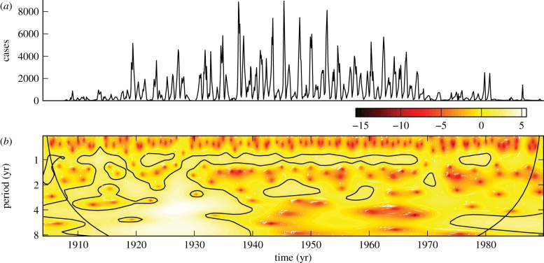
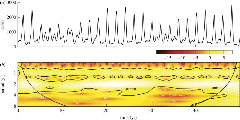
Figure 1a shows measles incidence in Ontario (1904–1989) and figure 1b shows the corresponding wavelet power spectrum. High-amplitude wavelet coefficients are isolated by dark contours and reveal a distinctive period 1 recurrence in the time series. An annual rise in infections is attributed to an increase in contact rates at the beginning of the school year [3,4], while the presence of significance contours at non-integer values of the period indicates non-seasonal recurrence [23]. After mass measles vaccination was introduced in the late 1960s, the number of cases dropped dramatically. A distinct decrease in the number of high-amplitude wavelet coefficients is apparent from the scalogram.

Figure 1.

(a) Reported monthly measles cases in Ontario, 1904–1989. (b) Corresponding wavelet power spectrum computed using the Morlet wavelet. The 95% confidence level (compared to Gaussian white noise) is indicated by black contours. The cone of influence indicates that part of the wavelet power spectrum that is contaminated by end effects. (Online version in colour.)

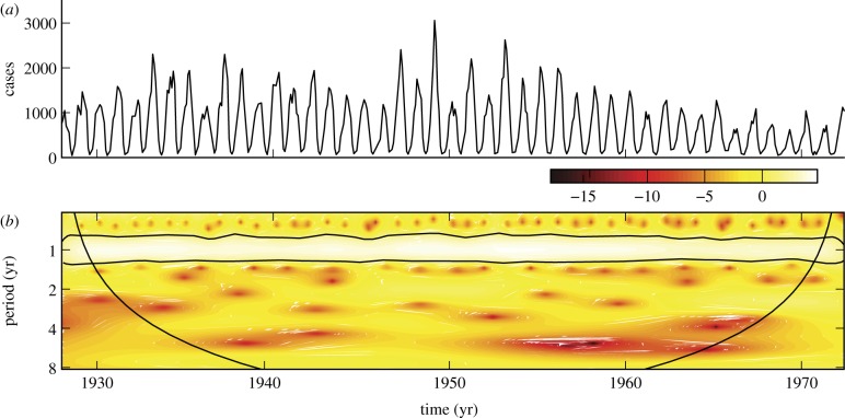
A strong yearly recurrence of chicken pox is unmistakable in figure 2. These monthly data were collected from 1928 to 1972 in New York City.

Figure 2.

(a) Reported monthly chicken pox cases in New York City, 1928–1972. (b) Corresponding wavelet power spectrum as in figure 1. (Online version in colour.)

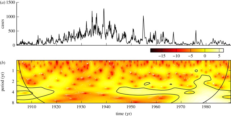
The incidence of whooping cough, as reported in Ontario from 1904 to 1989, is plotted in figure 3a. The wavelet scalogram in figure 3b demonstrates period 3–5-year recurrence after 1945.

Figure 3.

(a) Reported monthly whooping cough cases in Ontario, 1904–1989. (b) The corresponding wavelet power spectrum as in figure 1. (Online version in colour.)

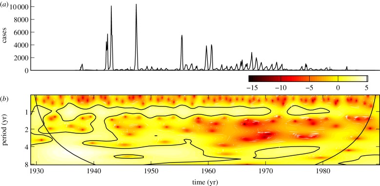
Figure 4a shows monthly incidence of rubella in Ontario from 1929–1989. The scalogram illustrates complex patterns of recurrence with both seasonal and non-seasonal peaks.

Figure 4.

(a) Reported monthly rubella cases in Ontario, 1929–1989. (b) The corresponding wavelet power spectrum as in figure 1. (Online version in colour.)

3.2. Simulated incidence time series

The WTMM method was also applied to incidence data generated by the standard stochastic SEIR epidemic model [7,24]. The SEIR model divides the host population into compartments containing susceptible (S), exposed (E), infectious (I) and recovered (R) individuals. Susceptibles have no immunity and can become infected upon contact with an infectious individual. Exposed individuals have been infected but are not yet infectious. Infectious individuals can infect susceptibles who they contact. Recovery is assumed to entail lifelong immunity. Assuming a mass-action contact process, the mean-field in the large population size limit [25] is governed by the standard deterministic SEIR model [7,26], which is specified by the following set of differential equations:

3.1a

3.1b

3.1c

3.1d

The total population size is . ν is the birth rate, which varies seasonally in reality [27] but is usually assumed constant or very slowly varying [4,28]. p is the proportion of individuals who are vaccinated before encountering infectious individuals. μ is the per capita death rate (from ‘natural’ causes; disease-induced mortality is negligible for the diseases we consider here). If , then N remains constant (which was true in our simulations). β is the transmission rate, which is typically time-varying for childhood infections (as a result of the aggregation of children in schools in term-time [3]). In our simulations, we used sinusoidal seasonal forcing

3.2

Thus, is the mean transmission rate and the amplitude of seasonality. Here σ is the (constant) rate at which exposed individuals become infectious (so the mean latent period is ). γ is the (constant) rate of recovery, so the mean infectious period is . The basic reproduction number, the average number of secondary infections caused by an infectious individual in a wholly susceptible population, is [7]

3.3

We implemented the stochastic SEIR model using the standard Gillespie algorithm [29] with event rates given by each of the terms in equations (3.1a–d). While the SEIR model ignores many aspects of real demographic and epidemiological interactions, it nevertheless successfully captures many features of real epidemics [7,28].

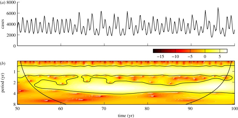
Figures 5 and 6 show simulation time series and wavelet power spectra for comparison with the reported incidence in the earlier figures. Figure 5 was generated with parameter values appropriate for measles (, days, days, amplitude of seasonal forcing ) and a population of two million. The scalogram in figure 5b exhibits the same period 1 recurrence observed for the Ontario measles data in figure 1, but shows significant period 2 recurrence which is not present in the Ontario data and does not exhibit the complexity of recurrence observed in Ontario over longer intervals of time.

Figure 5.

(a) Simulated weekly measles incidence, generated by the stochastic SEIR model with basic reproduction number , mean latent period days, mean infectious period days, seasonal amplitude and a population of million. (b) Corresponding wavelet power spectrum as in figure 1. (Online version in colour.)

Figure 6.

(a) Simulated weekly chicken pox cases, generated by the stochastic SEIR model with basic reproduction number , mean latent period days, mean infectious period days, seasonal amplitude and a population of . (b) Corresponding wavelet power spectrum as in figure 1. (Online version in colour.)

Figure 6 is based on a simulation of chicken pox dynamics (, days, days, ) and million. Again, significant period 1 coefficients reveal an annual pattern of recurrence in figure 6b. A similar pattern was observable from the reported incidence of chicken pox in New York City shown in figure 2.

4. Results

4.1. Analysis of incidence of infection time-series data

To select the optimal wavelet for the time series, we computed the singularity spectrum D(α) using Gaussian analysing wavelets of increasing order with . Figure 7a shows the spectra computed from the monthly Ontario measles incidence. The figure is a representative example of convergence results for measles data, but the location of the peak varies with geographical location. The fourth-order Gaussian wavelet was the lowest order Gaussian wavelet for which we observed convergence, and therefore was the optimal choice.

Figure 7.

Wavelet choice: the multifractal singularity spectra computed from (a) measles incidence of infection data reported monthly in Ontario, Canada, from 1904 to 1989 and (b) the number of chicken pox cases reported weekly in Ontario from 1925 to 1958. Gaussian wavelets were tested against the data using an increasing number of vanishing moments. The order of the wavelet and thus the number of vanishing moments of the wavelet is given by the number of derivatives of the Gaussian. (Online version in colour.)

Figure 7b shows that D(α) for weekly reported chicken pox in Ontario is also convergent, having similar peak locations and overall shapes for all orders of wavelets tested. All of the available chicken pox, whooping cough and rubella data also produced convergent spectra and confirmed that the fourth-order wavelet is an appropriate choice for comparisons of the observed time series.

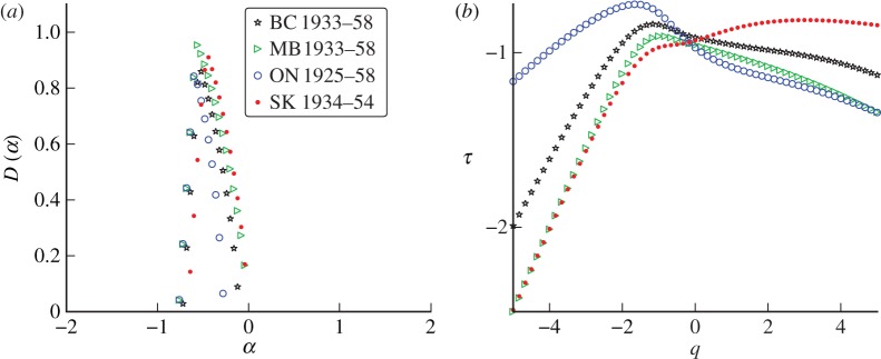
Figure 8 shows that the distribution of singularities is nearly identical for the chicken pox time series from British Columbia, Saskatchewan, Manitoba and Ontario. These results suggest that the nature of the disease itself may determine the shape of the singularity spectrum. We propose that this characteristic shape is the multifractal signature of the disease.

Figure 8.

(a) The singularity spectra for weekly chicken pox incidence in British Columbia (BC), Manitoba (MB), Ontario (ON) and Saskatchewan (SK). (b) The associated scaling functions. (Online version in colour.)

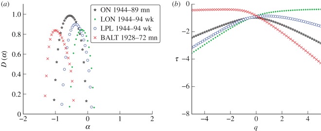
Figure 9 compares the singularity spectra for measles incidence in several widely separated geographical locations. This figure shows that measles incidence appears to have a distinctive singularity structure, regardless of location. All of the measles singularity spectra share the same qualitative features: they are all smooth on the top with a wide base (characteristic of a true multifractal statistical structure in time). This distinguishes the measles spectra from the chicken pox spectra which have pointed tops with a narrow base (suggestive of an approximately monofractal statistical structure in time). The scaling functions produced by the chicken pox datasets are more linear than those of measles. This indicates that chicken pox incidence is approximately monofractal, while measles incidence has a true multifractal structure (recall that τ(q) is a straight line for a true monofractal). Indeed, measles incidence appears to be more singular in structure than the chicken pox incidence, i.e. the peaks of the measles singularity spectra are generally located at smaller values of α.

Figure 9.

(a) Singularity spectra computed from reported measles incidence in Ontario, Canada (ON), London, UK (LON), Liverpool, UK (LPL), and Baltimore (BALT) in the USA. wk and mn refer to weekly and monthly data, respectively. (b) The associated scaling functions. (Online version in colour.)

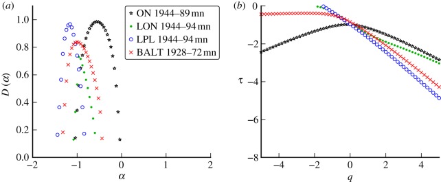
Figure 10 shows the same data as figure 9, but the weekly Liverpool and London time series have been aggregated four-weekly to approximate a monthly reporting interval. This temporal aggregation shifts the peak of the spectrum to the left and narrows the base of the spectrum (for both cities). It is evident from the comparison of figures 9 and 10 that changes in the reporting interval can have non-negligible effects on the singularity spectrum. Comparisons of different datasets should be made using the same (or a similar) reporting interval.

Figure 10.

(a) Effects of temporal aggregation of data on singularity spectra and (b) scaling functions. The weekly measles incidence data analysed in figure 9 were aggregated four-weekly to approximate monthly data. (Online version in colour.)

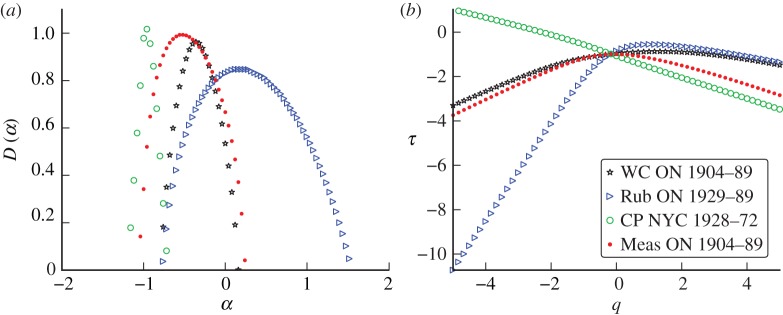
Extending the analysis to rubella and whooping cough reveals that each disease is characterized by a unique singularity structure as evinced by the qualitative differences between their respective singularity spectra. Figure 11 illustrates these differences between singularity spectra computed from monthly reported incidence. The qualitative shape of the whooping cough spectrum starkly contrasts the narrow pointed shape of the chicken pox spectrum and their associated scaling functions confirm that the former exhibits a broader multifractal structure. These comparisons, together with the very similar chicken pox spectra from different geographical locations, support the idea that each disease is characterized by a unique multifractal signature.

Figure 11.

(a) Singularity spectra computed from monthly incidence for several different diseases: whooping cough (WC), rubella (Rub), chicken pox (CP) and measles (Meas). (b) Scaling functions. (Online version in colour.)

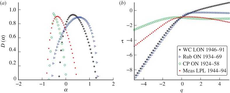
Comparisons of the spectra resulting from higher frequency (weekly) incidence from each of the diseases confirm the presence of such signatures and an example is presented in figure 12. These higher-frequency (weekly) whooping cough data produce a more distinctly multifractal spectrum than was observed in the monthly case. Again, each disease appears to have a unique singularity structure that can be identified qualitatively.

Figure 12.

(a) Singularity spectra for weekly reported cases of whooping cough (WC), rubella (Rub), chicken pox (CP) and measles (Meas). (b) Scaling functions. (Online version in colour.)

We propose that the singularity spectrum provides a distinctive signature that may be used to characterize different diseases based solely on a statistical analysis of incidence time series. An accurate numerical model should be able to reproduce this multifractal signature, at least qualitatively. In §4.2, we investigate whether the stochastic SEIR epidemic model, which is the standard mathematical model for the childhood diseases we have examined, is capable of reproducing the multifractal structure we have detected in the incidence data.

Previous work [4,23,28] has demonstrated that substantial changes in susceptible recruitment rates (determined by birth and vaccination rates) induce dynamical transitions. We therefore divided several time series into segments of approximately constant recruitment and recomputed the singularity spectra for each segment separately (we did this for whooping cough in London and measles in London and Liverpool). Our investigation into the effects of these dynamical transitions is restricted by the limitations of the WTMM method, which requires large numbers of data points to accurately measure the local regularity of a time series. For this reason, we considered only weekly data for this analysis.

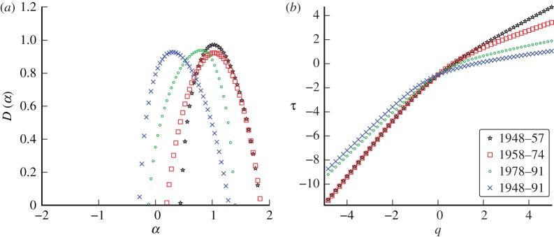
Changes in London whooping cough incidence were strongly influenced by the introduction of whole-cell vaccination in 1957 [30]. Figure 13 shows the singularity spectrum for each period of approximately constant susceptible recruitment. The main qualitative difference is that the peak location for the full time series is more negative (i.e. more singular) than the peak locations of those spectra generated by the divided regions. Although the peak locations vary slightly, the qualitative signature of the data is similar for all three time periods.

Figure 13.

(a) Singularity spectrum for whooping cough in London, UK, 1948–1991. The data are split into sections of roughly constant recruitment as described by Bauch & Earn [23]. (b) The scaling function. (Online version in colour.)

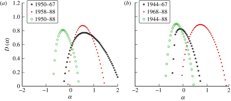
Figure 14 shows the singularity spectra for weekly measles incidence in London (figure 14a) and Liverpool (figure 14b). The partition of the data was determined by the time of introduction of measles vaccine. For Liverpool, the spectra for post-vaccination data lie further to the right (i.e. smoother) than for the pre-vaccination era. This suggests that the introduction of the vaccine caused the disease dynamics to become more regular. For London, the pre-vaccination spectrum is much broader (i.e. more multifractal) than the post-vaccination spectrum, but the peak location changes very little. This indicates that the introduction of the vaccine made the time series more monofractal (i.e. regularly irregular).

Figure 14.

(a) Singularity spectrum for measles in London, UK, 1950–1988. (b) Singularity spectrum for measles in Liverpool, UK, 1944–1988. Data are split into sections of roughly constant recruitment as described by Bauch & Earn [23]. (Online version in colour.)

The pre-vaccination spectra from London and Liverpool are qualitatively different. The reasons for these differences are unclear, though we note that the birth rate was much higher in Liverpool and that this induced an annual cycle of epidemics in Liverpool and a biennial cycle in London [4].

4.2. Singularity spectra of susceptible-exposed-infectious-recovered epidemic simulations

The WTMM method was applied to incidence time series generated by the stochastic SEIR epidemic model with parameters typical of measles in the pre-vaccination era (, days, days) and a population of 2 million people. For comparison with the reported data, the optimal analysing wavelet is found by computing the singularity spectra using increasing orders, n, of Gaussian analysing wavelets.

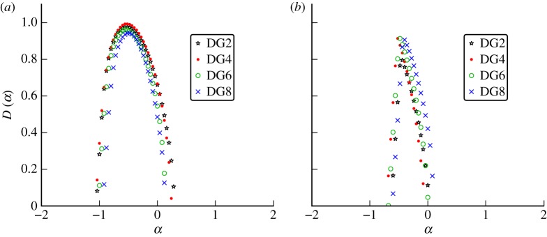
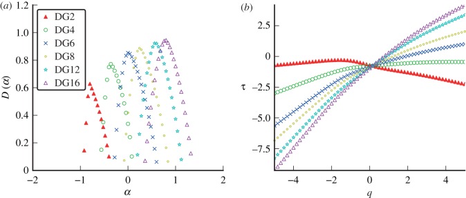
Figure 15 shows singularity spectra for simulated measles incidence with seasonal forcing amplitude . The spectrum shifts monotonically to the right as n increases from 2 to 16. The same result was found for simulations with other seasonal amplitudes . The spectrum clearly does not converge with increasing order of analysing wavelet, and much of the DG16 spectrum extends to , suggesting that large subsets of the signal are in fact continuous and differentiable.

Figure 15.

(a) Singularity spectra computed from measles simulations using wavelets from the Gaussian family. The amplitude of seasonal forcing was with a population of 2 million people. Derivatives of the Gaussian function are denoted DG and the order, or the number of derivatives taken, is the same as the number of vanishing moments of the wavelet. (b) The associated scaling functions. (Online version in colour.)

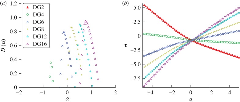
The optimal wavelet analysis was repeated for simulated chicken pox incidence with a population size of 10 million (, days, days) in figure 16. The regularity of the simulated chicken pox data varies significantly over time, so we have deliberately selected one of the less smooth regimes. Although the simulation spectra seem to share the pointed peak characteristic of real chicken pox data, the simulation data are much smoother. As for measles, the location of the peak of the singularity spectrum shifts monotonically to the right as the order of the Gaussian analysing wavelet increases.

Figure 16.

(a) Singularity spectra for SEIR simulations with chicken pox parameters. The amplitude of seasonal forcing was with a population of 10 million people. Derivatives of the Gaussian function are denoted DG and the order, or the number of derivatives taken, is the same as the number of vanishing moments of the wavelet. (b) The associated scaling functions. (Online version in colour.)

Since a wavelet of order n is capable of detecting singularities of order , the spectrum of a fractal signal is expected to converge to a unique spectrum once the highest order singularities present in the signal are resolved. Lack of convergence suggests that the simulated data are smoother than the analysing wavelets. For all of the simulated data, the scaling function becomes more linear with increasing n, which suggests that higher-order singularities are not present in the signal. The linearity of the scaling function, τ(q), usually indicates a monofractal structure, but the lack of convergence provides evidence that the data are dominated by smooth sub-intervals.

Mallat [9] proved that smooth perturbations of a multifractal signal introduce a bias in the singularity spectrum and proposed that this bias be detected by varying the order of the analysing wavelet, n. The presence of smooth sub-intervals can inhibit the tracking of WTMM lines (§2) causing the spectrum to vary with the order of the analysing wavelet.

Numerical tests of SEIR simulation data for a range of model parameters have confirmed the presence of smooth sub-intervals in the simulated time series. This behaviour is qualitatively different from the singularity spectra produced by the reported data shown in figure 7, which exhibits convergence with n. The time series generated by the stochastic SEIR model produces fewer high-amplitude wavelets coefficients at the finest scales, which further demonstrates that the simulated incidence data are significantly smoother than the reported incidence data.

Overall, our analysis strongly suggests that the time series produced by the stochastic SEIR epidemic model are only weakly singular and are unlikely to be multifractal or even monofractal. This contrasts sharply with the reported data, which are clearly multifractal and strongly singular. It appears that the stochastic SEIR epidemic model does not capture the singular multiscale time structure that characterizes the reported incidence data.

5. Discussion and conclusions

The WTMM multifractal formalism was used to analyse time series of reported cases of measles, chicken pox, whooping cough and rubella from a variety of geographical locations. A characteristic multifractal singularity spectrum was identified for each disease. Multiple datasets from different locations corresponding to the same disease produce singularity spectra with qualitatively similar shapes, which distinguish them from spectra associated with the other diseases (with some exceptions, e.g. measles in London versus Liverpool).

Table 2 shows that weekly incidence data for a given disease at different geographical locations have similar characteristics, while table 3 shows that weekly incidence data for different infectious diseases differ significantly in both their irregularity and their degree of multifractality. The peak Hölder exponent α ranges from −0.6 (indicating discontinuous data) to 0.6 (indicating continuous but non-differentiable data). The degree of multifractality, measured by the width of the singularity spectrum, ranges from 0.7 to 2.0. In fact, the chicken pox data seem to be approximately monofractal (all others are clearly multifractal).

Table 2.

Multifractal signatures of measles and chicken pox, presented as the peak positions and base widths of singularity spectra. Means and standard deviations were computed from monthly time series for four geographical locations for each disease (cf. figure 8 for chicken pox and figure 10 for measles).

disease	peak	width	type
chicken pox			approximately monofractal
measles			multifractal

Table 3.

Multifractal signatures based on a single weekly incidence time series for each disease (cf. figure 12).

disease	peak	width	type
chicken pox	−0.6	0.7	approximately monofractal
measles	−0.4	1.3	multifractal
rubella	0.6	2.0	multifractal
whooping cough	0.3	1.6	multifractal

Visual comparisons of time-series and conventional (periodicity) spectra of infectious disease incidence or mortality suggest that weekly or monthly counts of cases or deaths encode essential characteristics of different pathogens. However, converting such visual impressions into a formal statistic is not straightforward and has not been attempted to our knowledge. The approach we have presented in this paper suggests that infectious diseases have multifractal signatures, which are relatively easy to compute and provide a useful new way to describe infectious disease data. These signatures might, in certain cases, permit a disease to be identified purely on the basis of a statistical analysis of its reported incidence or mortality time series. This approach could be used, in principle, to confirm the cause of historical epidemics that have been identified by analysis of ancient DNA [31], to identify the causative agent of historical epidemics from which direct evidence cannot be obtained, or to help isolate the causes of transitions in disease dynamics that correlate with changes in the associated multifractal signature. Moreover, the WTMM method can be used as a new way of statistically validating models: accurate numerical simulations should reproduce the multifractal signatures of the diseases they are intended to model.

We used the WTMM technique to analyse simulated incidence data generated by the stochastic SEIR epidemic model. The simulated time series generated by the stochastic SEIR model were much smoother than the observed data for all of the diseases tested. In fact, by analysing the data with Gaussian wavelets of increasing order, we found that the singularity spectra do not even converge. This lack of convergence suggests that the simulated data generated by the stochastic SEIR model are dominated by smooth sub-intervals and do not capture the full multiscale structure of the real incidence data.

In particular, we found that real measles data are characterized by a broad (multifractal) singularity spectrum, but after testing a range of model parameters we concluded that the stochastic SEIR model could not reproduce such a spectrum, even qualitatively. Increasing the amplitude of seasonal forcing, , did improve the fit of the model's spectrum somewhat, but did not produce convergent spectra. We investigated the effect of parameter changes in the SEIR model and considered the effect of imperfect reporting in an attempt to better match the qualitative statistical properties of the real data, but without success.

The precise reasons behind the SEIR model's inability to produce multifractal, singular incidence data remain unclear. Possible reasons include stochastic fluctuations in the fundamental parameters of the disease (such as transmission rate), the existence of spatial hierarchies involving the interaction of urban centres of different sizes or time-varying differences between the actual incidence rate and the reported incidence rate. It is also possible that the dynamics of the stochastic SEIR model do not adequately capture the richness of the dynamical system governing the actual infectious disease transmission process.

Our analysis confirms that multiscale wavelet analysis offers powerful new tools for classifying infectious diseases based on their incidence time series and for qualitatively comparing and fitting models to reported data. Accurate mathematical models of infectious disease transmission are important for public health decision-makers, who can use models to design better control strategies. We have shown that, as measured by the singularity spectrum, the most popular epidemic model appears to miss some important multiscale time structure clearly present in the reported data. We hope that the results will lead to improved epidemic models, and a better understanding of the mechanisms underlying the spread of infectious disease.

References

- 1.Muller C. P., Kremer J. R., Best J. M., Dourado I., Triki H., Reef S. 2007. Reducing global disease burden of measles and rubella: report of the WHO Steering Committee on research related to measles and rubella vaccines and vaccination, 2005. Vaccine 25, 1–9 10.1016/j.vaccine.2006.07.039 (doi:10.1016/j.vaccine.2006.07.039) [DOI] [PubMed] [Google Scholar]
- 2.Bartlett M. S. 1960. Stochastic population models in ecology and epidemiology, vol. 4 Methuen's Monographs on Applied Probability and Statistics London, UK: Spottiswoode, Ballantyne & Co. Ltd [Google Scholar]
- 3.London W., Yorke J. A. 1973. Recurrent outbreaks of measles, chickenpox and mumps. I. Seasonal variation in contact rates. Am. J. Epidemiol. 98, 453–468 [DOI] [PubMed] [Google Scholar]
- 4.Earn D. J. D., Rohani P., Bolker B. M., Grenfell B. T. 2000. A simple model for complex dynamical transitions in epidemics. Science 287, 667–670 10.1126/science.287.5453.667 (doi:10.1126/science.287.5453.667) [DOI] [PubMed] [Google Scholar]
- 5.Alonso D., McKane A. J., Pascual M. 2007. Stochastic amplification in epidemics. J. R. Soc. Interface 4, 575–582 10.1098/rsif.2006.0192 (doi:10.1098/rsif.2006.0192) [DOI] [PMC free article] [PubMed] [Google Scholar]
- 6.Stone L., Olinky R., Huppert A. 2007. Seasonal dynamics of recurrent epidemics. Nature 446, 533–536 10.1038/nature05638 (doi:10.1038/nature05638) [DOI] [PubMed] [Google Scholar]
- 7.Anderson R. M., May R. M. 1991. Infectious diseases of humans: dynamics and control. Oxford, UK: Oxford University Press [Google Scholar]
- 8.Bacry E., Muzy J., Arneodo A. 1993. Singularity spectrum of fractal signals from wavelet analysis: exact results. J. Stat. Phys. 70, 635–674 10.1007/BF01053588 (doi:10.1007/BF01053588) [DOI] [Google Scholar]
- 9.Mallat S. 1998. A wavelet tour of signal processing. Burlington, MA: Academic Press [Google Scholar]
- 10.Jaffard S. 1997. Multifractal formalism for functions. II. Self-Similar functions. SIAM J. Math. Anal. 28, 971–998 10.1137/S0036141095283005 (doi:10.1137/S0036141095283005) [DOI] [Google Scholar]
- 11.Ivanov P. C., Amaral L. A., Goldberger A. L., Havlin S., Rosenblum M. G., Struzik Z. R., Stanley H. E. 1999. Multifractality in human heartbeat dynamics. Nature 399, 461–465 10.1038/20924 (doi:10.1038/20924) [DOI] [PubMed] [Google Scholar]
- 12.West B. J., Latka M. 2005. Fractional Langevin model of gait variability. J. Neuroeng. Rehabil. 2, 24–33 10.1186/1743-0003-2-24 (doi:10.1186/1743-0003-2-24) [DOI] [PMC free article] [PubMed] [Google Scholar]
- 13.Song I. H., Lee S. M., Kim I. Y., Lee D. S., Kim S. I. 2005. In Multifractal analysis of electroencephalogram time series in humans. Lecture Notes in Computer Science, pp. 921–926 Berlin, Germany: Springer [Google Scholar]
- 14.Shimizu Y., Barth M., Windischberger C., Mose E., Thurner S. 2004. Wavelet-based multifractal analysis of fMRI time series. Neuroimage 22, 1195–202 10.1016/j.neuroimage.2004.03.007 (doi:10.1016/j.neuroimage.2004.03.007) [DOI] [PubMed] [Google Scholar]
- 15.Chiu K. M., Chan H. L., Chu S. H., Lin T. Y. 2007. Carvedilol can restore the multifractal properties of heart beat dynamics in patients with advanced congestive heart failure. Auton. Neurosci. Basic Clin. 132, 76–80 10.1016/j.autneu.2006.10.008 (doi:10.1016/j.autneu.2006.10.008) [DOI] [PubMed] [Google Scholar]
- 16.Bauch C. T. 2008. The role of mathematical models in explaining recurrent outbreaks of infectious childhood diseases. Math. Epidemiol. 1945, 297–319 10.1007/978-3-540-78911-6_11 (doi:10.1007/978-3-540-78911-6_11) [DOI] [Google Scholar]
- 17.Grenfell B. T., Kappey J., Bjornstad O. N. 2001. Travelling waves and spatial hierarchies in measles epidemics. Nature 414, 716–723 10.1038/414716a (doi:10.1038/414716a) [DOI] [PubMed] [Google Scholar]
- 18.Torrence C., Compo G. P. 1998. A practical guide to wavelet analysis. Bull. Am. Meteorol. Soc. 4, 415–447 See http://www.inference.phy.cam.ac.uk/mackay/PhD.html. [Google Scholar]
- 19.Hurst H. E. 1951. Long-term storage capacity of reservoirs. Trans. Am. Soc. Civ. Eng. 116, 770–808 [Google Scholar]
- 20.Donoho D., Maleki A., Shahram M. 2007. WaveLabe850. See www-stat.stanford.edu/wavelab [Google Scholar]
- 21.Mallat S., Hwang W. L. 1992. Singularity detection and processing with wavelets. IEEE Trans. Inf. Theory 38, 617–643 10.1109/18.119727 (doi:10.1109/18.119727) [DOI] [Google Scholar]
- 22.IIDDA The International Infectious Disease Data Archive. See http://iidda.mcmaster.ca. [Google Scholar]
- 23.Bauch C., Earn D. 2003. Transients and attractors in epidemics. Proc. R. Soc. Lond. B 270, 1573–1578 10.1098/rspb.2003.2410 (doi:10.1098/rspb.2003.2410) [DOI] [PMC free article] [PubMed] [Google Scholar]
- 24.Bailey N. T. J. 1975. The mathematical theory of infectious diseases and its applications, 2nd edn. New York, NY: Hafner Press [Google Scholar]
- 25.Kurtz T. G. 1980. Relationships between stochastic and deterministic population models. Lect. Notes Biomath. 38, 449–467 10.1007/978-3-642-61850-5_39 (doi:10.1007/978-3-642-61850-5_39) [DOI] [Google Scholar]
- 26.Kermack W. O., McKendrick A. G. 1927. A contribution to the mathematical theory of epidemics. Proc. R. Soc. Lond. A 115, 700–721 10.1098/rspa.1927.0118 (doi:10.1098/rspa.1927.0118) [DOI] [Google Scholar]
- 27.He D., Earn D. J. D. 2007. Epidemiological effects of seasonal oscillations in birth rates. Theor. Popul. Biol. 72, 274–291 10.1016/j.tpb.2007.04.004 (doi:10.1016/j.tpb.2007.04.004) [DOI] [PubMed] [Google Scholar]
- 28.Earn D. J. D. 2009. Mathematical epidemiology of infectious diseases. In Mathematical biology, vol. 14 (eds Lewis M. A., Chaplain M. A. J., Keener J. P., Maini P. K.), pp. 151–186 Providence, RI: IAS/Park City, Mathematics Series American Mathematical Society [Google Scholar]
- 29.Gillespie D. T. 1976. A general method for numerically simulating the stochastic time evolution of coupled chemical reactions. J. Comput. Phys. 22, 403–434 10.1016/0021-9991(76)90041-3 (doi:10.1016/0021-9991(76)90041-3) [DOI] [Google Scholar]
- 30.Rohani P., Earn D., Grenfell B. 1999. Opposite patterns of synchrony in sympatric disease metapopulations. Science 286, 968–971 10.1126/science.286.5441.968 (doi:10.1126/science.286.5441.968) [DOI] [PubMed] [Google Scholar]
- 31.Bos K. I., et al. 2011. A draft genome of Yersinia pestis from victims of the Black Death. Nature 478, 506–510 10.1038/nature10549 (doi:10.1038/nature10549) [DOI] [PMC free article] [PubMed] [Google Scholar]