Real time forecasting of near-future evolution

Abstract

A metaphor for adaptation that informs much evolutionary thinking today is that of mountain climbing, where horizontal displacement represents change in genotype, and vertical displacement represents change in fitness. If it were known a priori what the ‘fitness landscape’ looked like, that is, how the myriad possible genotypes mapped onto fitness, then the possible paths up the fitness mountain could each be assigned a probability, thus providing a dynamical theory with long-term predictive power. Such detailed genotype–fitness data, however, are rarely available and are subject to change with each change in the organism or in the environment. Here, we take a very different approach that depends only on fitness or phenotype–fitness data obtained in real time and requires no a priori information about the fitness landscape. Our general statistical model of adaptive evolution builds on classical theory and gives reasonable predictions of fitness and phenotype evolution many generations into the future.

1. Introduction

An intuitive association exists between the notions of quantitative science and predictive science. Biology's accelerating shift into the quantitative realm thus brings with it attendant expectations of predictive powers. Yet evolutionary biology, the discipline built on biology's most distinguishing process, has been famously silent on the matter of prediction [1,2], and this silence persists despite a well-established quantitative foundation.

Some observations may help us to explain this silence: (i) mutation, the ultimate source of heritable genetic novelty that feeds evolution, is the result of random replication infidelity that is unpredictable, (ii) fitnesses of newly arising mutations can be highly contingent on genetic background and are thus thought to be very unpredictable, (iii) environments, both abiotic and biotic, can change in unpredictable ways, changing fitnesses of existing variants as well as newly arising mutations, (iv) the trajectories and fates of newly arising mutant lineages are strongly affected by random sampling (genetic drift) and (v) recombination crossovers, despite having hotspots on the genome, can occur at random positions.

These considerations, and others, have understandably given rise to the established (and sometimes celebrated [2]) position that evolution is inherently unpredictable [1]. Evidence in support of this position has been claimed in palaeontology [3,4] (but see [5]), molecular evolution [6], long-term evolutionary studies [7], experimental evolution [8,9] and even in silico evolution [10,11]; such evidence, however, typically takes unpredictability to be the null hypothesis and merely reports a failure to reject this null, leaving ample room for type II error. Other evidence is less clear, showing mixed results and reaching ambiguous conclusions [12–14]. In contrast, some work finds clear evidence of parallel evolution in experimental [13,15–17] and natural [18] populations; i.e. in retrospect, the evolution of these populations had a degree of predictability. Finally, there are a handful of papers that entertain the notion of predicting evolution in a prospective way and speculate how this might be achieved [12,19–21], especially in the context of the influenza virus [22–25].

Predicting the future course of evolution requires a model. We focus on evolutionary models and thus do not consider purely statistical time-series models. Evolutionary models that may be applied to the problem of predicting evolution can be divided into two categories: (i) ‘fitness landscape’ or ‘adaptive topography’ models [26–31] that focus on the mutational input to adaptation and largely ignore, or statistically summarize, the net effects of [32–36], the population dynamics of adaptation and (ii) ‘adaptive process’ models [37–40] that focus on the population dynamics of adaptation; most of these either ignore or make simplistic assumptions about the mutational input to adaptation. (We note that there are some models that resist this simple categorization, cf. [41–43].)

Adaptive topography approaches to predicting evolution are well-suited to long-term prediction, because they map out the mutations underlying the often slow ‘adaptive walk’ of populations; however, there are two significant difficulties with this approach: (i) adaptive topographies are usually contingent on many factors and the assumption of their long-term stasis, implicit in most such models (but see [44,45]), is thus questionable at best, and (ii) mapping out potentially adaptive mutations requires either a vast amount of genotype–fitness data or it requires the experimental evolution of a test population [20]. Acquiring an exhaustive genotype–fitness map is so time-consuming and labour-intensive that this approach cannot rightly be said to offer real time prediction. Furthermore, identifying adaptive mutations through such maps or through a priori experimental evolution offers predictions that are not truly prospective in nature.

In light of the significant difficulties with adaptive topography methods, we would argue that a first step towards predicting evolution should implement an adaptive process approach. In what follows, we re-derive a standard evolutionary model that describes the adaptive process and even allows for mutational input in a very general way. We then apply standard transforms to this model resulting in a cumulant expansion (a hierarchy of statistical relations), which can be used to predict evolution in real time, with no a priori information about the organism in question or its environment.

Predicting the near-future course of evolution based on these statistical relations is then achieved in three steps: first, a number of fitness or phenotype–fitness measurements are taken from the population in question; these are taken from a number of individuals sampled from the population at one or more time points. Second, these measurements are inserted into the statistical relations to infer the mutational input that feeds ongoing evolution, i.e. mutation rate and distribution of mutational effects. Third, a discretization of the statistical relations gives rise to a telescoping algorithm for projecting the statistical properties of fitness or a fitness-related phenotype into the near future. Using this method, we have succeeded in predicting the future course of in silico evolution (fully stochastic simulations) roughly 40 generations into the future.

Our approach differs from many previous discussions of predicting evolution in that we start at a very elemental level: (i) we ask first how the evolution of fitness itself might be forecast, (ii) we then ask how the evolution of a fitness-related phenotype might be forecast and (iii) we soberly aspire to predict evolution only tens of generations into the future. While the developments presented here offer only a rudimentary beginning, they offer the novel prospect of a theoretical framework onto which more comprehensive prediction algorithms might be built.

2. Methods

2.1. Assumptions and general model description

We present and analyse a standard model of fitness evolution. We focus on the most general form of this model that makes no asymptotic assumptions and no assumptions about the shapes of the fitness or mutational distributions. In what follows, the word ‘fitness’ will mean ‘haploid fitness’ or ‘additive genic fitness’. Extension to diploid and polyploid organisms is discussed later. The continuous function u(x,t) is defined such that, at time t, the fraction of individuals in the population whose fitness lies in the interval (x,x + dx) becomes identically equal to u(x,t)dx in the limit as dx approaches zero. The deterministic convergence to u(x,t)dx reflects underlying assumptions of infinite population size and infinitely divisible fitness. The model is conservative and thus ensures that the fitness distribution at any given time is a probability density, i.e. , for all t. In what follows, we refer to the group of individuals whose fitness lies in the interval (x,x + dx) as ‘fitness class x’.

An example fitness distribution might look something like that illustrated in figure 1, where the histogram represents frequencies of individuals in different fitness bins in a finite population, and the solid line represents the continuous approximation of that distribution. The arrows indicate the different evolutionary ‘forces’ acting on this distribution. The distribution in this illustrative figure is randomly multimodal, and perhaps even a bit improbable, in order to emphasize the point that no assumptions restrict the shape, smoothness or previous dynamics of the distribution. The analysis begins by making the continuous approximation (solid line), but a comparison with individual-based stochastic simulations demonstrates that the results obtained using the continuous approximation can apply quite well to finite populations (histogram).

Figure 1.

An illustration of the different evolutionary forces that shape the fitness distribution of a population. The histogram represents a finite population and the solid curve represents the corresponding infinite population approximation.

2.2. Model of fitness evolution

To model selection, we assume that the per capita growth rate of individuals with fitness x is equal to the relative fitness of those individuals, , where is mean fitness, i.e. 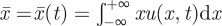. To model mutational influx, fitness class x grows in weighted proportion to the sizes of neighbouring fitness classes. The weights depend on the overall mutation rate and on the distance from a given point to x; they are prescribed by the distribution of fitness-effects of mutations, g(γ,t), where γ is the horizontal distance from x, and g(γ,t) is a probability density, i.e. for all t. Mutational influx is thus modelled by the convolution where μ is genomic mutation rate. Mutational outflux is modelled as a decrease in fitness class x in direct proportion to the size of that fitness class: . Summing the effects of selection and mutation gives rise to a general equation for fitness dynamics:

2.1

This evolutionary model is not new. The equation expresses, in continuous mathematical form, an evolutionary model that has been expressed previously in continuous mathematical, discrete mathematical and verbal form. The model, in the exact form taken in equation (2.1), has been studied previously [41]. In discrete form, it has been dubbed the ‘replicator equation’ [46] and used to describe and study viral ‘quasi-species’ [37,47–49]. In verbal form, it has been conjectured numerous times and may be as old as evolutionary theory itself.

2.3. Statistical properties of fitness evolution

Our analysis of equation (2.1) uses slight variations on standard transforms. We first transform equation (2.1) to central-moment-generating function (cmgf) form; the cmgf is defined as (essentially equivalent to a Laplace transform). Next, the equation is transformed to central-cumulant-generating function (ccgf) form, defined as . We define M(θ,t) to be the moment-generating function (mgf) for the distribution of mutational effects, g(γ,t). Then the transformed equation for evolutionary dynamics is

2.2

where subscripts denote partial derivatives with respect to the subscripted variable, and , the rate of fitness increase or adaptation rate. From this transformed equation, the following unclosed hierarchy of equations is immediate:

2.3

where κ_j = κ_j(t) denotes the jth central cumulant of the fitness distribution at time t (central cumulants are functions of central moments), , the rate of change of the jth central cumulant, and m_j = m_j (t) denotes the jth raw moment of the underlying fitness-effect distribution of newly arising mutations. Fitness measurements from a population can give estimates for the κ_i, which can then be inserted into these equations. In a more general context, equation (2.3) was derived previously by Bürger [41].

2.4. Model of phenotype evolution

Here, we model the evolution of a fitness-related phenotype. The continuous function u(z,x,t) is defined such that, at time t, the fraction of individuals in the population whose fitness lies in the interval (x,x + dx) and whose phenotype lies in the interval (z,z + dz) becomes identically equal to u(z,x,t)dx dz in the limit as dx and dz approach zero. Again, the model is conservative and thus ensures that the fitness–phenotype distribution at any given time is a probability density.

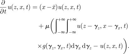
Again, per capita growth rate of individuals with fitness x is equal to the relative fitness of those individuals, , where is the mean fitness, i.e. . The mutational influx is given by the convolution , where μ is the genomic mutation rate. The mutational outflux is . Summing the effects of selection and mutation gives rise to an equation for phenotype dynamics:

2.4

2.5. Statistical properties of phenotype evolution

We analyse equation (2.4) by first transforming it to cmgf form; the cmgf is defined as . Next, the equation is transformed to ccgf form, defined as . The transformed evolutionary equation is

2.5

where , the rate of increase in mean phenotype, and again , the rate of fitness increase. In a way similar to previous derivations, but now in two spatial dimensions, the dynamic fitness–phenotype distribution is characterized by this set of equations:

2.6

where κ_i,j = κ_i,j(t) denotes the (i,j)th central cumulant of the fitness distribution at time t, the rate of change of the (i,j)th central cumulant, and m_ij = m_ij(t) denotes the (i,j)th raw moment of the underlying fitness-effect distribution of newly arising mutations. Fitness–phenotype measurements from a population can give estimates for the κ_i,j, which can then be inserted into these equations. We note that setting i = 1 gives the dynamics of mean phenotype , a fact we will use later under §3.1.

2.6. Refinements

2.6.1. Ploidy and recombination

For organisms whose ploidy is n > 1, equations (2.3) and (2.6) may be approximated as follows: (i) account for masking effects by replacing the κ_j+1 or κ_i,j+1 on the right-hand side by sκ_j+1 or sκ_i,j+1, where is a strength-of-selection factor (the first of these replacements was also noted previously by Burger [41]), and (ii) replace μm_j by or μm_i,j by , respectively, where , the de novo contribution of dominance to the jth moment in an n-ploid organism, where λ_i is the gradient of mean dominance of the ith ploid (or gene segment copy, in the case of segmented viruses) with respect to fitness (see the electronic supplementary material). The foregoing analyses apply when the unit of selection is either the entire genome, if it is haploid, or the ‘gene’ if ploidy is n > 1. It may be the case that recombination occurs within the unit of selection, especially if the unit of selection is the entire genome. When such intra-unit recombination occurs at a high rate with no net effect of dominance, its effects may be approximated by adding the term and to the right-hand side of all but the first relation in equations (2.3) and (2.6), respectively, where r is the recombination rate and π_j is the jth central moment of the fitness distribution and π_i,j is the (i,j)th central moment of the phenotype–fitness distribution.

2.6.2. Epistasis

The foregoing analyses allow mutational input to be time-dependent. While this approach should capture most mutational dynamics reasonably well, it may miss certain aspects attributable to the contingency of mutational effects on genetic background, or epistasis. We account for epistasis by assuming that the fitness effects of newly arising mutations are a function, not only of time but also of the fitness of the genetic background onto which the mutations arise. We define δ_j to be the gradient of the jth moment of the mutational effects distribution with respect to fitness. Then, the moments m_j and m_i,j in equations (2.3) and (2.6) are simply replaced by

and

respectively, where the m_j and m_i,j now denote ‘baseline’ moments (see the electronic supplementary material). These baseline moments may be functions of time, reflecting a distribution of mutational effects that is both time-dependent and contingent on genetic background.

3. Results

3.1. Predicting evolution

The foregoing statistical relations may be used to predict the near-future course of evolution, following the three steps outlined in §1. To avoid unnecessary repetition, in much of what follows, we treat the cases of fitness and phenotype evolution in parallel. Results pertaining to fitness evolution derive from equation (2.3), while results pertaining to phenotype evolution derive from equation (2.6). While we give the procedure to estimate phenotype–fitness mutational input quite generally, i.e. for all the two-dimensional moments (μm_i,j for all (i,j)), we focus only on predicting the evolution of mean phenotype after that; this is achieved by setting i = 1 and limiting the equations to μm_1,j and κ_1,j. The Discussion outlines the generalization that projects the full distribution.

3.1.1. The necessary measurements

Predicting the future course of fitness evolution requires fitness measurements taken from several individuals in the population. As a minimal requirement, several such measurements must be taken at a single time point, namely, the present. To make predictions based on such minimal data, it requires two assumptions: (i) that the mutational input to evolution does not change over time, and (ii) that the fitness distribution has converged to a constant shape that simply propagates towards increased fitness. These two ‘dynamic equilibrium’ assumptions, while somewhat questionable, may provide a reasonable first approximation; indeed, adaptive evolution under this regime, called the ‘solitary wave’ of adaptation, has been studied appreciably [50–54]. To relax these assumptions, fitness measurements must be taken at the present time and at one or more time points in the past; now, predictions do not rely on the ‘dynamic equilibrium’ assumptions described earlier but on the less-restrictive single assumption that mutational input follows unknown but generally characterizable trends.

Predicting the future evolutionary course of a fitness-related phenotype requires measurements of both the fitness and the phenotype of several individuals in the population. As with the fitness-only predictions described earlier, and for the same reasons outlined there, it is preferable to have measurements taken at the present time and at one or more time points in the past.

3.1.2. Inferring mutational input

Data taken from a single time point. As indicated already, evolutionary predictions can be made based on measurements from only a single sample taken at the present time; however, this relies on the two ‘dynamic equilibrium’ assumptions described earlier. The second of these two assumptions translates to the conditions and in equation (2.3) (c_x is constant) for the case of fitness evolution; and it translates to the conditions and in equation (2.6) (c_z is constant) for the case of phenotype evolution. Applying these conditions to equations (2.3) and (2.6) directly gives the quantities μm_j or μm_i,j that characterize the fitness or phenotype–fitness mutational input, respectively:

3.1

where

Data taken from more than one time point. Using data taken from more than one time point, we can relax the questionable ‘dynamic equilibrium’ assumptions described earlier. This is achieved simply by a coarse discretization of equations (2.3) and (2.6). The quantities μm_j or μm_i,j (now dynamic) are thus estimated as follows:

3.2

where Δt is the sampling interval, and everything else on the right-hand side of the equations is obtainable from the fitness or phenotype–fitness measurements. No asymptotic assumptions are required here, and the dynamics of the distribution of mutational effects can thus be studied by estimating μm_j = μm_j(t) or μm_i,j = μm_i,j(t) at different time points during the evolution of a population.

We note that mutation rate cannot be estimated separately in the earlier-mentioned non-parametric scheme (only the products μm_j(t) and μm_i,j(t) can be estimated). Furthermore, if recombination is present and r is to be estimated too, then there is one too many parameters, i.e. the system of equations is under-determined. To remedy this, it may be assumed that the underlying distribution, g(γ,t) or g(γ_z,γ_x,t), has a certain form (making the problem parametric); this can result in a well-determined or over-determined system that can, in principle, be used to estimate μ, r and the parameters of the now-parametric underlying distribution, a method we have tested with some success.

Comparing estimates of μm_i and μm_i,j to their known values in simulations. As a first means to evaluate the theory developed here, we employed the foregoing estimation procedures on virtual data from fully stochastic simulations of populations undergoing adaptive evolution and compared these estimates with the known values that were put into the simulations. Figure 2 plots the results of one such comparison for fitness evolution and one for phenotype evolution.

Figure 2.

Assessing inference of mutational input. Absolute values of the μm_j and μm_1,j. Known values (solid lines), calculated from the parameters of the simulations, follow the curve. Circles show the averages of values estimated from equation (3.2). In the individual-based stochastic simulations, deleterious mutation rate was 0.1, beneficial mutation rate was 0.0001, effects of mutations were drawn from an exponential distribution with mean 0.03 and population size was 10 000. (a) Fitness evolution and (b) phenotype evolution.

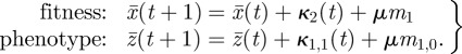
3.1.3. Projecting the near-future course of evolution

With the estimates of μm_i or μm_1,j in hand, we have the information necessary to project near-future evolution. Here again, we employ a discretization of equations (2.3) and (2.6), but this discretization is much less coarse than that used to determine mutational input. The first equation becomes

3.3

This gives mean fitness only one generation from now (where ‘now’ is time t). The formula for mean fitness (or mean phenotype) two generations from now is

3.4

where (or ) have already been calculated in equation (3.3). To complete this calculation, however, we need a predicted value for κ₂(t + 1) (or κ_1,1(t + 1)); this is obtained from discretizing the second expression in equations (2.3) and (2.6), which gives:

3.5

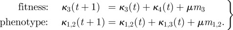
To predict mean fitness (or mean phenotype) three generations from now, we use

3.6

where and are obtained from equation (3.4), and κ₂(t + 2) and κ_1,1(t + 2) are obtained from

3.7

where

3.8

And so on. In general, this iterative ‘telescoping’ procedure can be written compactly as

3.9

for , where R is the predictive reach of the algorithm. In practice, the hierarchy of equations cannot be infinite, and there must be some j_max at which the system of equations is closed (equivalent to the problem of moment closure). To close the system of equations, we suppose that and , thereby closing the system of equations with this last equation:

3.10

3.2. Testing predictions against simulations

As a first step towards assessing the accuracy of our methods for predicting evolution, we wrote simulations to mimic evolving populations. These simulations kept track of every individual and every replication event in the population. Offspring could differ from parents in fitness. At the outset, every individual in the population had a fitness of one and the wild-type genomic mutation rate set by the user.

3.2.1. Mechanics of the simulations

At each time step, every individual produced a number of offspring, X, drawn at random from a Poisson distribution whose mean was , where w_i is the fitness of the ith individual in the population and is the mean fitness of the population. Each offspring acquired: (i) a number X_D of new deleterious mutations that each decreased fitness by a factor (1−M_D), (ii) a number X_B of new beneficial mutations that each increased fitness by a factor (1 + M_B). X_D and X_B are Poisson random variables with means μf_D, μf_B, respectively, where μ is the base genomic mutation rate, and the f's are fractions of deleterious and beneficial mutations, respectively—parameters set by the user. To simulate mutational effects, M_D ≥ 0 and M_B ≥ 0 were continuous random variables with means m_D, and m_B, respectively. These methods were employed for figure 2. Parameter values for most simulations were chosen to reflect the adaptive regime of some experimental evolution populations [55,56]: population size and beneficial mutation rate were well into the ‘clonal interference’ regime of adaptive evolution, in which several competing beneficial mutations are likely to co-exist in the population at any given time.

To mimic a static environment in which the degree of adaptedness changes over time, and to assess predictive accuracy under these non-asymptotic conditions, some simulations implemented a limited supply of beneficial mutations (figures 3–6). This was achieved by considering all beneficial mutations to reside on a finite, indeed small, ‘beneficial genome’, modelled as a string of ones and zeros, i.e. a ‘bit-string’ genome. Figures 3 and 4 plot example simulations (blue curves) and predictions based on ‘data’ taken from those simulations for the near-future course of evolution (red curves).

Figure 3.

Predictions for fitness evolution. Blue line plots the fitness trajectory of the simulated population; red lines plot predicted fitness trajectories based on our telescoping method. The data used for the telescoping method are: a sample of 100 fitness measurements taken from the population at the start of each red line, and second sample of 100 fitness measurements taken 100 generations prior to that (to estimate the μm_j(t)). Green lines plot the extrapolated predictions of Fisher's theorem [39], and the light blue line in the inset plots the extrapolated prediction of Kimura's related equation [57] (the F/K equation; see §4). Parameters for the simulations are the same as those given in figure 2, except here the supply of beneficial mutations is limited (there are 64 available at the outset) and is thus used up as the population evolves.

Figure 6.

Improvement over F/K projections. We employ simulations to assess the predictive accuracy of our methods by comparing it to the accuracy of linear extrapolations of F/K predictions (see §4). Simulations were fully stochastic and individual-based; deleterious mutation rate was 0.05, beneficial mutation rate was 0.0001, effects of mutations were drawn from an exponential distribution with mean 0.03. Circles indicate that a population size of 10 000 was used; squares indicate that a population size of 50 000 was used. Filled indicates that the entire population was sampled to compute the cumulants; empty indicates that cumulants were calculated from a sample of size 100 taken from the population. Values plotted are computed from 400 non-overlapping prediction-assessment intervals of 50 generations each, taken from two simulated evolving populations, each with a non-renewable supply of 96 beneficial mutations that is used up as the population adapts. (a) The r.m.s.e. of F/K projections (r.m.s.e.(F/K)) minus the r.m.s.e. of our fitness forecasting method (r.m.s.e.(FF)), quantifying the improvement in predictive accuracy of our methods over F/K projections. Curiously, these curves follow a power-law (solid curves) with exponents 1.82 (whole population) and 1.86 (sample size 100). (b) Probabilities supporting the null hypothesis (p-values) that our methods perform no better than F/K projections. These values were calculated using the non-parametric sign test as suggested by Diebold & Mariano [61], which if anything should err on the conservative side.

Figure 4.

Predictions for phenotype evolution. Blue line plots the fitness trajectory of the simulated population; red lines plot predicted phenotype trajectories based on our telescoping method. The predictions made, using our method (red lines), are based on one set of 100 phenotype–fitness measurements taken from the population at the start of each red line, and a second set of 100 phenotype–fitness measurements taken 100 generations prior to that (to get current estimates of the μm_1,j(t)). Green lines plot the extrapolated predictions of the Price equation, and the light blue line in the inset plots the extrapolated prediction of the full Price equation [40,58,59]. Parameters for the simulations are the same as those given in figure 2, except for the distribution of mutational effects, which is a two-dimensional Gaussian distribution in fitness and phenotype with means (−0.03, −0.08) and covariance matrix .

3.2.2. Assessing predictive accuracy of our methods

Taking a lead from meteorology, we employed normalized root-mean-square error (r.m.s.e.) as our indicator of predictive accuracy, given by the formula:

where is the ith predicted value for mean fitness, is the ith observed value for mean fitness, and are maximum and minimum observed mean fitness. Figure 5 shows how this indicator of predictive accuracy is affected by population size. As expected, our methods perform much better when selection is the ‘limiting step’ to evolution (empty symbols, figure 5), i.e. in the ‘clonal interference’ regime [60]; they do not perform as well when mutation is the limiting step (filled circles, figure 5), i.e. in the ‘periodic selection’ regime.

Figure 5.

Effect of population size on predictive accuracy. Normalized r.m.s.e. of predictions (see text) is plotted as a function of time into the future that predictions are made. Predictions are compared against individual-based simulations in which deleterious mutation rate was μf_D = 0.05, beneficial mutation rate was μf_B = 5 × 10⁻⁵, and fitness effects of mutations were drawn from an exponential distribution with mean 0.03. Different symbols indicate different population sizes and different corresponding quantities F = 2N μf_B log(Ns/2) indicating the adaptive regime [60]: filled circles indicate a population of size n = 1000 that is in the periodic selection regime (F = 0.27 < 1); empty circles and empty rectangles indicate populations of size n = 10 000 and n = 100 000 that are in the clonal interference regime (F = 5.01 > 1 and F = 73.13 ≫ 1, respectively).

The difficulty with a straight comparison between observed data and predicted values, as plotted in figure 5, is that there is no obvious way to formulate a null hypothesis representing ‘inaccurate prediction’, whose rejection would thereby support ‘accurate prediction’. To quantitatively assess predictive accuracy, therefore, we compared our predictions with those of the ‘next best’ predictor, which is linear extrapolation of the Fisher/Kimura (F/K) equation (figure 6), given by the equation , where is mean fitness projected t generations into the future, is variance in additive fitness measured at the present time, t = 0 (the ‘Fisher term’), and μm₁ is the genomic mutation rate times the mean effect of mutations on additive fitness based on present and perhaps past data (the ‘Kimura term’). Figure 6 shows that improvement of our methods over F/K projections can increase with decreasing population size. This is because, while our methods are less accurate in smaller populations, the F/K projections are also less accurate; the amount by which the accuracy of our methods is reduced in a smaller population may be less than the amount by which F/K projections are reduced, so the improvement of our methods over F/K projections can be larger in a small population. Figure 6b shows that these improvements are highly significant and that their significance increases with time.

4. Discussion

We note that when there is no mutation, i.e. when μ = 0, the fitness equations (equation (2.3)) reduce to the set of relations: , the first of which is Fisher's fundamental theorem of natural selection, (adhering to our definition of x as additive genic fitness). This celebrated relation states that the instantaneous rate of increase of mean fitness equals the fitness variance; it is an exact but dynamically insufficient result [62]. If it were known how the variance were changing over time at the same instant, this could slightly extend our knowledge of the future trajectory of mean fitness, thereby incrementally increasing the dynamical sufficiency of Fisher's theorem. The rate of change in fitness variance is precisely what is given by the second relation, ; this rate in turn depends on the third cumulant, whose rate of change is given by the next equation, , and so on. In this way, the effects of the higher cumulants percolate down through the equations, ultimately extending the projected dynamics of mean fitness in a telescoping fashion. This observation suggests that predictions for the trajectory of mean fitness may be extended beyond that predicted by Fisher's theorem, and it might be viewed as adding a degree of dynamical sufficiency to Fisher's theorem. This is the logic behind our method for forecasting the near-future course of fitness evolution. When mutation is added, the full system is that given by equation (2.3), the first of which is analogous to Kimura's more general equation [57]. And just as with Fisher's theorem, equation (2.3) might be viewed as adding a degree of dynamical sufficiency to the Kimura equation.

In a similar fashion, when there is no mutation and setting i = 1, the phenotype equations (equation (2.6)) reduce to the set of relations: , the first of which is the Price equation [40], (adhering again to our definition of x as additive fitness): the instantaneous rate of change of a fitness-related phenotype equals the covariance between fitness and phenotype. Like Fisher's theorem, it is an exact but dynamically insufficient result [58]. And just as the equations for the higher (one-dimensional) cumulants allow the future projection of mean fitness beyond that predicted by Fisher's theorem, the equations for the higher two-dimensional cumulants allow the future projection of mean phenotype beyond that predicted by the Price equation. This is the logic behind our method for forecasting the near-future course of phenotype evolution. When mutation is added, the full system is that given by equation (2.6), the first of which is analogous to the ‘full’ Price equation [40,58,59]. And just as with the Price equation, the hierarchy of expressions in equation (2.6) might be viewed as adding a degree of dynamical sufficiency to the full Price equation.

Figures 3 and 4 plot two typical examples of evolutionary trajectories from fully stochastic, individual-based simulations, compared with the predicted trajectories calculated using the telescoping method described earlier. As points of comparison to classical theory, figure 3 also plots the predictions of Fisher's ‘fundamental theorem’, as well as the related Kimura equation (extrapolated beyond their one-generation reach for illustration); figure 4 also plots the predictions of the Price equation, as well as the ‘full’ Price equation (also extrapolated beyond their one-generation reach for illustration).

In principle, the telescoping method we describe can be used to predict not only the future trajectory of mean fitness or mean phenotype but also the future dynamics of the full fitness or phenotype distribution: equation (3.9) gives not only mean fitness or mean phenotype at time τ, but it also gives the higher cumulants at time τ. We have not exploited this fact in the current paper. It may be desirable, for example, to predict not only the future adaptedness of a population (indicated by its mean fitness) but also its future ‘adaptive capacity’ (or adaptation rate); this latter quantity is given by κ₂(τ) in equation (3.9). To project the future course of evolution for the entire phenotype marginal distribution, the general form of equation (3.9) may be written compactly as for all i ≥ 1 and j ≥ 0. This allows projection of the κ_i,0, for all i ≥ 1, which uniquely projects the future dynamics of the full marginal distribution of the phenotype.

Our analyses and statistical models implicitly assume infinite population size, a fact that is reflected by the absence of a parameter N for population size. We suspect that this assumption is quite weak for our purposes, because of the timescales involved. This suspicion is corroborated by the observations (i) that predictions based on the continuous (infinite N) approximation appear to work quite well with simulated data from finite N populations, and (ii) the improvement over F/K projections is actually slightly greater for a smaller population size (figure 6). The most significant error introduced by the infinite N assumption comes about because, in an infinite population, all possible fitness variants—even variants with very high fitness—are present at all times, even if at miniscule frequency. When a model based on this assumption is applied to finite populations, it allows for the growth of minute fractions of individuals, which is of course a biological absurdity. The most significant consequence of this absurdity is that high fitness variants can grow, under the infinite population assumption, even when they do not yet exist in a finite population. (Consequentially, it has been shown [51] that the infinite population assumption leads to unboundedly accelerating fitness increase, whereas a finite population with the same parameters shows a linear fitness increase.) However, the error introduced by the infinite population assumption typically takes a considerable amount of time to affect predictions. To illustrate, we imagine a population of 10⁵ individuals whose fitnesses follow a normal distribution with mean one and standard deviation 0.05. A fitness variant with selective advantage 4 pre-exists in the infinite population model, but it exists at such a low frequency that it would require 797 generations for that variant to reach a frequency of 10⁻⁵, which would correspond to a single individual in our finite population of 10⁵. This number of generations is much greater than the current predictive reach of our model. We are nevertheless concerned that the error introduced by the infinite population assumption may limit the predictive reach of our methods, and we are currently exploring application of previous work that remedies these limitations: (i) employing a right-truncated fitness distribution with a ‘stochastic edge’, as outlined by Rouzine et al. [50,53,54], and (ii) employing a tuning technique for evolutionary models introduced by Hallatschek [52] that absorbs the stochastic effects of finite N.

In addition to accounting for the effects of finite N, future work will address the related issues of how to determine an appropriate time interval, given the real data. Furthermore, we plan to perform a more rigorous evaluation of the predictability provided by our methods as well as a comprehensive sensitivity analysis. Finally, we are planning to test this theory with evolving in vitro populations of Escherichia coli. We have already completed pilot experiments (K. Sprouffske, C. Gentile, P. Sniegowski, & P. Gerrish 2012, unpublished data), which indicate that a strong signature of predictability can be obtained using the methods outlined here with a modest amount of experimental work.

As mentioned in the Introduction, the present study offers a rudimentary beginning to the problem of predicting evolution. While the focus of this study has been the evolution of fitness or a fitness-related phenotype, most applications of this work will be more complex and will seek ways to predict the evolution of multiple phenotypes or genotypic features. The cumulant expansion presented here is easily extended to n phenotypic or genotypic dimensions. Such an extension could potentially predict the trajectories and perhaps fates of n existing polymorphisms; however, its applicability to de novo phenotypes or genotypic features is questionable and a subject for further study.

Notably, our results carry no asymptotic requirements and apply equally well to recently perturbed populations that are far from dynamic equilibrium. As time progresses, our model also allows for changes in the mutational landscape through the dynamic mutational term; this term can accommodate epistatic contingencies as long as they admit of statistical characterization. Eventually, however, the dynamics of mutational effects and contingencies will surely resist further prospective characterization, a fact that will limit the timescale of applicability.

References

- 1.Mayr E. 1988. Toward a new philosophy of biology: observations of an evolutionist. Cambridge, MA: Harvard University Press [Google Scholar]
- 2.Scriven M. 1959. Explanation and prediction in evolutionary theory. Science 130, 477–482 10.1126/science.130.3374.477 (doi:10.1126/science.130.3374.477) [DOI] [PubMed] [Google Scholar]
- 3.Gould S. J. 1989. Wonderful life: the Burgess Shale and the nature of history, 1st edn New York, NY: W.W. Norton [Google Scholar]
- 4.Simpson G. G. 1950. Evolutionary determinism and the fossil record. Sci. Mon. 71, 262–267 [Google Scholar]
- 5.Conway Morris S. 1998. The crucible of creation: the Burgess Shale and the rise of animals. Oxford, UK: University Press [Google Scholar]
- 6.Monod J., Wainhouse A. 1972. Chance and necessity: an essay on the natural philosophy of modern biology. London, UK: Collins [Google Scholar]
- 7.Grant P. R., Grant B. R. 2002. Unpredictable evolution in a 30-year study of Darwin's finches. Science 296, 707–711 10.1126/science.1070315 (doi:10.1126/science.1070315) [DOI] [PubMed] [Google Scholar]
- 8.Blount Z. D., Borland C. Z., Lenski R. E. 2008. Historical contingency and the evolution of a key innovation in an experimental population of Escherichia coli. Proc. Natl Acad. Sci. USA 105, 7899–7906 10.1073/pnas.0803151105 (doi:10.1073/pnas.0803151105) [DOI] [PMC free article] [PubMed] [Google Scholar]
- 9.Woods R. J., Barrick J. E., Cooper T. F., Shrestha U., Kauth M. R., Lenski R. E. 2011. Second-order selection for evolvability in a large Escherichia coli population. Science 331, 1433–1436 10.1126/science.1198914 (doi:10.1126/science.1198914) [DOI] [PMC free article] [PubMed] [Google Scholar]
- 10.Yedid G., Bell G. 2002. Macroevolution simulated with autonomously replicating computer programs. Nature 420, 810–812 10.1038/nature01151 (doi:10.1038/nature01151) [DOI] [PubMed] [Google Scholar]
- 11.Gerrish P. 2002. Computation biology: evolution plays dice. Nature 420, 756–757 10.1038/420756a (doi:10.1038/420756a) [DOI] [PubMed] [Google Scholar]
- 12.Bull J. J., Molineux I. J. 2008. Predicting evolution from genomics: experimental evolution of bacteriophage T7. Heredity 100, 453–463 10.1038/sj.hdy.6801087 (doi:10.1038/sj.hdy.6801087) [DOI] [PubMed] [Google Scholar]
- 13.Nakatsu C. H., Korona R., Lenski R. E., de Bruijn F. J., Marsh T. L., Forney L. J. 1998. Parallel and divergent genotypic evolution in experimental populations of Ralstonia sp. J. Bacteriol. 180, 4325–4331 [DOI] [PMC free article] [PubMed] [Google Scholar]
- 14.Wichman H. A., Badgett M. R., Scott L. A., Boulianne C. M., Bull J. J. 1999. Different trajectories of parallel evolution during viral adaptation. Science 285, 422–424 10.1126/science.285.5426.422 (doi:10.1126/science.285.5426.422) [DOI] [PubMed] [Google Scholar]
- 15.Cunningham C. W., Jeng K., Husti J., Badgett M., Molineux I.J., Hillis D. M., Bull J. J. 1997. Parallel molecular evolution of deletions and nonsense mutations in bacteriophage T7. Mol. Biol. Evol. 14, 113–116 [DOI] [PubMed] [Google Scholar]
- 16.Bull J. J., Badgett M. R., Wichman H. A., Huelsenbeck J. P., Hillis D. M., Gulati A., Ho C., Molineux I. J. 1997. Exceptional convergent evolution in a virus. Genetics 147, 1497–1507 [DOI] [PMC free article] [PubMed] [Google Scholar]
- 17.Wood T. E., Burke J. M., Rieseberg L. H. 2005. Parallel genotypic adaptation: when evolution repeats itself. Genetica 123, 157–170 10.1007/s10709-003-2738-9 (doi:10.1007/s10709-003-2738-9) [DOI] [PMC free article] [PubMed] [Google Scholar]
- 18.Hohenlohe P. A., Bassham S., Etter P. D., Stiffler N., Johnson E. A., Cresko W. A. 2010. Population genomics of parallel adaptation in threespine stickleback using sequenced RAD Tags. PLoS Genet. 6, e1000862. 10.1371/journal.pgen.1000862.t003 (doi:10.1371/journal.pgen.1000862.t003) [DOI] [PMC free article] [PubMed] [Google Scholar]
- 19.Bairoch A., Murzin A. 1997. Sequences and topology: predicting evolution. Curr. Opin. Struct. Biol. 7, 367–368 10.1016/S0959-440X(97)80053-X (doi:10.1016/S0959-440X(97)80053-X) [DOI] [PubMed] [Google Scholar]
- 20.Hall B. G. 2002. Predicting evolution by in vitro evolution requires determining evolutionary pathways. Antimicrob. Agents Chemother. 46, 3035–3038 10.1128/AAC.46.9.3035-3038.2002 (doi:10.1128/AAC.46.9.3035-3038.2002) [DOI] [PMC free article] [PubMed] [Google Scholar]
- 21.Reeve J. P. 2000. Predicting long-term response to selection. Genet. Res. 75, 83–94 10.1017/S0016672399004140 (doi:10.1017/S0016672399004140) [DOI] [PubMed] [Google Scholar]
- 22.Bush R. M., Bender C. A., Subbarao K., Cox N. J., Fitch W. M. 1999. Predicting the evolution of human influenza A. Science 286, 1921–1925 10.1126/science.286.5446.1921 (doi:10.1126/science.286.5446.1921) [DOI] [PubMed] [Google Scholar]
- 23.Plotkin J. B., Dushoff J., Levin S. A. 2002. Hemagglutinin sequence clusters and the antigenic evolution of influenza A virus. Proc. Natl Acad. Sci. USA 99, 6263–6268 10.1073/pnas.082110799 (doi:10.1073/pnas.082110799) [DOI] [PMC free article] [PubMed] [Google Scholar]
- 24.Huang J.-W., Yang J.-M. 2011. Changed epitopes drive the antigenic drift for influenza A (H3N2) viruses. BMC Bioinform. 1(Suppl. 12), S31. 10.1186/1471-2105-12-S1-S31 (doi:10.1186/1471-2105-12-S1-S31) [DOI] [PMC free article] [PubMed] [Google Scholar]
- 25.Liao Y. C., Lee M. S., Ko C. Y., Hsiung C. A. 2008. Bioinformatics models for predicting antigenic variants of influenza A/H3N2 virus. Bioinformatics 24, 505–512 10.1093/bioinformatics/btm638 (doi:10.1093/bioinformatics/btm638) [DOI] [PubMed] [Google Scholar]
- 26.Mustonen V., Kinney J., Callan C.G., Jr, Lässig M. 2008. Energy-dependent fitness: a quantitative model for the evolution of yeast transcription factor binding sites. Proc. Natl Acad. Sci. USA 105, 12 376–12 381 10.1073/pnas.0805909105 (doi:10.1073/pnas.0805909105) [DOI] [PMC free article] [PubMed] [Google Scholar]
- 27.Poelwijk F. J., Kiviet D. J., Weinreich D. M., Tans S. J. 2007. Empirical fitness landscapes reveal accessible evolutionary paths. Nature 445, 383–386 10.1038/nature05451 (doi:10.1038/nature05451) [DOI] [PubMed] [Google Scholar]
- 28.Rokyta D. R., Joyce P., Caudle S. B., Wichman H. A. 2005. An empirical test of the mutational landscape model of adaptation using a single-stranded DNA virus. Nat. Genet. 37, 441–444 10.1038/ng1535 (doi:10.1038/ng1535) [DOI] [PubMed] [Google Scholar]
- 29.Macken C. A., Perelson A. S. 1989. Protein evolution on rugged landscapes. Proc. Natl Acad. Sci. USA 86, 6191–6195 10.1073/pnas.86.16.6191 (doi:10.1073/pnas.86.16.6191) [DOI] [PMC free article] [PubMed] [Google Scholar]
- 30.Perelson A. S., Macken C. A. 1995. Protein evolution on partially correlated landscapes. Proc. Natl Acad. Sci. USA 92, 9657–9661 10.1073/pnas.92.21.9657 (doi:10.1073/pnas.92.21.9657) [DOI] [PMC free article] [PubMed] [Google Scholar]
- 31.Beardmore R. E., Gudelj I., Lipson D. A., Hurst L. D. 2011. Metabolic trade-offs and the maintenance of the fittest and the flattest. Nature 472, 342–346 10.1038/nature09905 (doi:10.1038/nature09905) [DOI] [PubMed] [Google Scholar]
- 32.Joyce P., Rokyta D. R., Beisel C. J., Orr H. A. 2008. A general extreme value theory model for the adaptation of DNA sequences under strong selection and weak mutation. Genetics 180, 1627–1643 10.1534/genetics.108.088716 (doi:10.1534/genetics.108.088716) [DOI] [PMC free article] [PubMed] [Google Scholar]
- 33.Orr H. A. 1998. The population genetics of adaptation: the distribution of factors fixed during adaptive evolution. Evolution 52, 935–949 10.2307/2411226 (doi:10.2307/2411226) [DOI] [PubMed] [Google Scholar]
- 34.Rokyta D. R., Beisel C. J., Joyce P. 2006. Properties of adaptive walks on uncorrelated landscapes under strong selection and weak mutation. J. Theor. Biol. 243, 114–120 10.1016/j.jtbi.2006.06.008 (doi:10.1016/j.jtbi.2006.06.008) [DOI] [PubMed] [Google Scholar]
- 35.Rokyta D. R., Beisel C. J., Joyce P., Ferris M. T., Burch C. L., Wichman H. A. 2008. Beneficial fitness effects are not exponential for two viruses. J. Mol. Evol. 67, 368–376 10.1007/s00239-008-9153-x (doi:10.1007/s00239-008-9153-x) [DOI] [PMC free article] [PubMed] [Google Scholar]
- 36.Rozen D. E., de Visser J. A. G. M., Gerrish P. J. 2002. Fitness effects of fixed beneficial mutations in microbial populations. Curr. Biol. 12, 1040–1045 10.1016/S0960-9822(02)00896-5 (doi:10.1016/S0960-9822(02)00896-5) [DOI] [PubMed] [Google Scholar]
- 37.Eigen M. 1971. Selforganization of matter and the evolution of biological macromolecules. Naturwissenschaften 58, 465–523 10.1007/BF00623322 (doi:10.1007/BF00623322) [DOI] [PubMed] [Google Scholar]
- 38.Domingo E., et al. 1985. The quasispecies (extremely heterogeneous) nature of viral RNA genome populations: biological relevance: a review. Gene 40, 1–8 10.1016/0378-1119(85)90017-4 (doi:10.1016/0378-1119(85)90017-4) [DOI] [PubMed] [Google Scholar]
- 39.Fisher R. A. 1930. The genetical theory of natural selection. Oxford, UK: Clarendon Press [Google Scholar]
- 40.Price G. R. 1970. Selection and covariance. Nature 227, 520–521 10.1038/227520a0 (doi:10.1038/227520a0) [DOI] [PubMed] [Google Scholar]
- 41.Bürger R. 1991. Moments, cumulants, and polygenic dynamics. J. Math. Biol. 30, 199–213 10.1007/BF00160336 (doi:10.1007/BF00160336) [DOI] [PubMed] [Google Scholar]
- 42.Jones A. G., Arnold S. J., Bürger R. 2007. The mutation matrix and the evolution of evolvability. Evolution 61, 727–745 10.1111/j.1558-5646.2007.00071.x (doi:10.1111/j.1558-5646.2007.00071.x) [DOI] [PubMed] [Google Scholar]
- 43.Turelli M. 1990. Dynamics of polygenic characters under selection. Theor. Popul. Biol. 38, 1–57 10.1016/0040-5809(90)90002-D (doi:10.1016/0040-5809(90)90002-D) [DOI] [Google Scholar]
- 44.Mustonen V., Lässig M. 2009. From fitness landscapes to seascapes: non-equilibrium dynamics of selection and adaptation. Trends Genet. 25, 111–119 10.1016/j.tig.2009.01.002 (doi:10.1016/j.tig.2009.01.002) [DOI] [PubMed] [Google Scholar]
- 45.Mustonen V., Lässig M. 2010. Fitness flux and ubiquity of adaptive evolution. Proc. Natl Acad. Sci. USA 107, 4248–4253 10.1073/pnas.0907953107 (doi:10.1073/pnas.0907953107) [DOI] [PMC free article] [PubMed] [Google Scholar]
- 46.Page K., Nowak M. 2002. Unifying evolutionary dynamics. J. Theor. Biol. 219, 93–98 [PubMed] [Google Scholar]
- 47.Briones C., Domingo E. 2008. Minority report: hidden memory genomes in HIV-1 quasispecies and possible clinical implications. AIDS Rev. 10, 93–109 [PubMed] [Google Scholar]
- 48.Domingo E., Baranowski E., Ruiz-Jarabo C. M., Martin-Hernandez A. M., Saiz J. C., Escarmis C. 1998. Quasispecies structure and persistence of RNA viruses. Emerg. Infect. Dis. 4, 521–527 10.3201/eid0404.980402 (doi:10.3201/eid0404.980402) [DOI] [PMC free article] [PubMed] [Google Scholar]
- 49.Mateu M. G., Martinez M. A., Rocha E., Andreu D., Parejo J., Giralt E., Sobrino F., Domingo E. 1989. Implications of a quasispecies genome structure: effect of frequent, naturally occurring amino acid substitutions on the antigenicity of foot-and-mouth disease virus. Proc. Natl Acad. Sci. USA 86, 5883–5887 10.1073/pnas.86.15.5883 (doi:10.1073/pnas.86.15.5883) [DOI] [PMC free article] [PubMed] [Google Scholar]
- 50.Rouzine I. M., Wakeley J., Coffin J. M. 2003. The solitary wave of asexual evolution. Proc. Natl Acad. Sci. USA 100, 587–592 10.1073/pnas.242719299 (doi:10.1073/pnas.242719299) [DOI] [PMC free article] [PubMed] [Google Scholar]
- 51.Tsimring L. S., Levine H., Kessler D. A. 1996. RNA virus evolution via a fitness-space model. Phys. Rev. Lett. 76, 4440–4443 10.1103/PhysRevLett.76.4440 (doi:10.1103/PhysRevLett.76.4440) [DOI] [PubMed] [Google Scholar]
- 52.Hallatschek O. 2011. The noisy edge of traveling waves. Proc. Natl Acad. Sci. USA 108, 1783–1787 10.1073/pnas.1013529108 (doi:10.1073/pnas.1013529108) [DOI] [PMC free article] [PubMed] [Google Scholar]
- 53.Brunet E., Rouzine I. M., Wilke C. O. 2008. The stochastic edge in adaptive evolution. Genetics 179, 603–620 10.1534/genetics.107.079319 (doi:10.1534/genetics.107.079319) [DOI] [PMC free article] [PubMed] [Google Scholar]
- 54.Rouzine I. M., Brunet E., Wilke C. O. 2008. The traveling-wave approach to asexual evolution: Muller's ratchet and speed of adaptation. Theor. Popul. Biol. 73, 24–46 10.1016/j.tpb.2007.10.004 (doi:10.1016/j.tpb.2007.10.004) [DOI] [PMC free article] [PubMed] [Google Scholar]
- 55.Gerrish P. J., Lenski R. E. 1998. The fate of competing beneficial mutations in an asexual population. Genetica 102/103, 127–144 10.1023/A:1017067816551 (doi:10.1023/A:1017067816551) [DOI] [PubMed] [Google Scholar]
- 56.Perfeito L., Fernandes L., Mota C., Gordo I. 2007. Adaptive mutations in bacteria: high rate and small effects. Science 317, 813–815 10.1126/science.1142284 (doi:10.1126/science.1142284) [DOI] [PubMed] [Google Scholar]
- 57.Kimura M. 1958. On the change of population fitness by natural selection. Heredity 12, 145–167 10.1038/hdy.1958.21 (doi:10.1038/hdy.1958.21) [DOI] [Google Scholar]
- 58.Gardner A. 2008. The Price equation. Curr. Biol. 18, R198–202 10.1016/j.cub.2008.01.005 (doi:10.1016/j.cub.2008.01.005) [DOI] [PubMed] [Google Scholar]
- 59.Frank S. A. 1995. George Price's contributions to evolutionary genetics. J. Theor. Biol. 175, 373–388 10.1006/jtbi.1995.0148 (doi:10.1006/jtbi.1995.0148) [DOI] [PubMed] [Google Scholar]
- 60.Sniegowski P. D., Gerrish P. J. 2010. Beneficial mutations and the dynamics of adaptation in asexual populations. Phil. Trans. R. Soc. B 365, 1255–1263 10.1098/rstb.2009.0290 (doi:10.1098/rstb.2009.0290) [DOI] [PMC free article] [PubMed] [Google Scholar]
- 61.Diebold F. X., Mariano R. S. 1995. Comparing predictive accuracy. J. Bus. Econ. Stat. 13, 253–263 10.2307/1392185 (doi:10.2307/1392185) [DOI] [Google Scholar]
- 62.Frank S. A., Slatkin M. 1992. Fisher's fundamental theorem of natural selection. Trends Ecol. Evol. 7, 92–95 10.1016/0169-5347(92)90248-a (doi:10.1016/0169-5347(92)90248-a) [DOI] [PubMed] [Google Scholar]