Prediction of invasion from the early stage of an epidemic

Abstract

Predictability of undesired events is a question of great interest in many scientific disciplines including seismology, economy and epidemiology. Here, we focus on the predictability of invasion of a broad class of epidemics caused by diseases that lead to permanent immunity of infected hosts after recovery or death. We approach the problem from the perspective of the science of complexity by proposing and testing several strategies for the estimation of important characteristics of epidemics, such as the probability of invasion. Our results suggest that parsimonious approximate methodologies may lead to the most reliable and robust predictions. The proposed methodologies are first applied to analysis of experimentally observed epidemics: invasion of the fungal plant pathogen Rhizoctonia solani in replicated host microcosms. We then consider numerical experiments of the susceptible–infected–removed model to investigate the performance of the proposed methods in further detail. The suggested framework can be used as a valuable tool for quick assessment of epidemic threat at the stage when epidemics only start developing. Moreover, our work amplifies the significance of the small-scale and finite-time microcosm realizations of epidemics revealing their predictive power.

1. Introduction

Predictability of catastrophic events such as earthquakes, epidemics, fracture or financial crashes [1–3] is a topic of increasing interdisciplinary interest. The predictability of these events is inextricably linked to the inherent complexity of the phenomena under consideration [1,2]. Here, we focus on epidemiology. Within this context, many studies have been devoted to prediction of the temporal incidence of epidemics (i.e. the evolution of the number of infected hosts in the course of an epidemic) [4–8]. Recently, an increasing number of papers have also considered the prediction of the spatio-temporal evolution of epidemics [9–12].

Both the temporal and the spatio-temporal incidence depend on complex factors related to the transmission of infection and the properties of the hosts. For instance, the hosts are not identical in susceptibility and transmissibility of infection owing to difference in age, size, genotype and neighbourhood. [5,9,10,13]. The transmission of infection is stochastic, meaning that a healthy host is infected by contact with inoculum from an infected host with a certain probability only. Many epidemics, notably those involving transmission by invertebrate vectors, or by wind and rain for many plant pathogens, are subject to variability in weather. This environmental stochasticity can also influence the evolution of epidemics in such heterogeneous systems [14]. All these factors make prediction of disease incidence an extremely challenging and sometimes controversial task [4,15,16]. Medley [4] suggests that, although obtaining precise quantitative predictions for the incidence would be obviously desirable, qualitative predictions may be more valuable. This is very much along the lines of ideas from the science of complexity claiming that, despite the fact that giving accurate predictions for the detailed evolution of complex systems might be an illusory task, certain qualitative features of the evolution, such as occurrence or absence of a catastrophic event, could be more amenable for prediction [2,17,18].

Here, we address the question of predictability of epidemics using a methodological framework inspired by the science of complexity. The main aim is to estimate the probability that an emerging epidemic will invade a significant fraction of the population in the future. This quantity can be viewed as a qualitative feature of the complete spatio-temporal evolution of epidemics.

We propose several methods for approaching the problem that offer different levels of precision. Our results suggest that the most precise methods do not necessarily lead to more reliable predictions. Instead, parsimony seems to be the key ingredient for prediction based on inherently limited observations. The framework presented below deals with epidemics caused by a broad class of pathogens leading to permanent immunity of infected hosts after recovery (or death). There are numerous examples of such diseases affecting populations of humans [19,20], animals [21] and plants [22]. The advantage in analysis of such epidemics is that they are characterized by a well-defined final state consisting of only hosts that were never infected and hosts that were infected and became immune. In particular, we focus on the estimation of the probability that an epidemic is invasive in the final state.

The proposed methods are first applied to prediction of invasion of a pathogen in an experimental model system in which the fungal plant pathogen, Rhizoctonia solani, spreads through a population of hosts represented by discrete nutrient sites. The properties of the sites, e.g. nutrient concentration, can be varied for different realizations of epidemics. Such a system is convenient for generation and observation of rapid, highly replicated and repeatable epidemics and it is used as a benchmark for description of our methodologies and analyses. The epidemic prediction analysis for the experimental system is followed by a test of our methods in numerical experiments for epidemics spreading on networks of hosts arranged on a regular lattice. The advantage of investigating such epidemics is that their properties are known beforehand and this allows us to provide a precise analysis of the performance of prediction methods by comparing with the expected behaviour.

2. Methods

The methods follow four steps that are basic for any scientifically meaningful prediction of the behaviour of a complex system: (i) observation of the initial evolution of the process over a certain period of time, t_obs; (ii) construction of a model for description of the observed behaviour; (iii) fitting the model to the data obtained from observations; and (iv) extrapolation of the behaviour to the future by using the model with the fitted parameters. These steps are interconnected and we argue that they should be kept at a similar level of complexity in order to make their interplay as consistent as possible. In this paper, we investigate whether or not such consistency is important for obtaining reliable predictions by exploring several combinations of strategies for steps (i)–(iii) (see summary in table 1).

Table 1.

Overview of methods for prediction. (Combination of possible datasets considered in step (i) and methods used for addressing steps (ii) and (iii) in the prediction process. The first column introduces a label for each set of methods, which are ordered according to their overall expected precision. The second column gives the format of the data obtained from observations in step (i). The smallest precision of the data corresponds to methods A and B in which only the incidence, C(t), is used. Methods C–E use a limited spatio-temporal knowledge of the evolution of the infection given by the shell-evolution function F(l,t). Method F uses the time of infection of each host, {t_i}, which is typically unknown from observations but can be inferred in step (iii). In step (ii), RF and CT are abbreviations for the Reed–Frost and continuous-time model, respectively. In step (iii), we have used several methods for fitting: minimum distance (MD), approximate Bayesian computation (ABC), and data-augmented Markov chain Monte Carlo (DA-MCMC). Column five lists the parameters involved in each step for prediction of the fungal invasion in the agar-dot experiment. Methods based on the RF dynamics are parametrized by the transmissibility, T, and a time scale . The CT dynamics used in methods E and F is parametrized by T, a characteristic time τ₀, and a shape parameter for the time-dependence of the transmission of infection, k. The RF dynamics corresponds to the limit k → ∞ of the CT dynamics. The MD method for fitting consists in minimizing the parameter d² (last column), which measures the difference between observations and numerical simulations. The ABC fitting procedure assumes that a simulated invasion fits well the observed epidemic if d² < ɛ, where ɛ is a free parameter. As shown in the last column, the definition of d² depends on the descriptors for observations used in step (i). For methods A and B, d² is defined in terms of the observed and simulated incidences, and , normalized to the number of hosts in the population, N. In methods C–E, d² is defined in terms of the shell-evolution function for observations and simulations. Sections I and II of the electronic supplementary material appendix S1 give more details on the definition of models used in step (ii) and fitting methods used in step (iii).)

methodology	step (i): data	step (ii): model	step (iii): fitting	parameters	d2
A	mean field (MF), C(t)	RF	MD	(ii)
B		RF	ABC	(ii) (iii) ɛ
C	shell,	RF	MD	(ii)
D		RF	ABC	(ii) (iii) ɛ
E		CT		(ii) T,τ0, k. (iii) ɛ
F	site, {ti }	CT	DA-MCMC	(i) {ti} (ii) T,τ0, k

For concreteness, we illustrate our prediction methods for the particular case of fungal colony invasion in microcosms comprising populations of nutrient sites (agar dots) [23]. In these experiments, the central agar dot in ensembles with the geometry shown in figure 1 was inoculated by the soil-borne fungal plant pathogen R. solani and the spread of the fungal colony is scored in discrete time steps (e.g. daily).

Figure 1.

Steps for prediction used in methodology C (table 1). (a(i)) Discrete spatio-temporal observations of evolution (spatio-temporal map) of a hypothetical epidemic spreading from the central host in a population of hosts (circles) arranged on a triangular lattice with lattice spacing a and L hosts per side of the hexagonal boundaries of the system. The arrangement of nutrient sites in the fungal invasion experiment analysed below is of this type. Numbers inside the circles denote the times, t = 0,1, … , of infection of hosts by the observation time t_obs = 2. Empty circles correspond to healthy (susceptible) hosts by the same time. The hexagons with dotted lines indicate the shells of hosts at a given chemical distance, l, to the centre of the system. (a(ii)) The spatio-temporal evolution of the epidemic is described by the shell-evolution function giving the relative number of hosts in layer l infected by time t. For instance, F(2,2) = 3/12 for the epidemic shown in (a(i)). (b) In step (ii), the epidemic is described in terms of a susceptible–infected–removed (SIR) model. An infected host, , remains infectious during the infectious period τ which, for simplicity, is taken as being constant over the whole population and set as a unit of time, τ = 1. After the infectious period τ, the host is removed, . During the time τ, can transmit the infection to a neighbouring susceptible host, , with probability T (transmissibility). Alternatively, can be removed without passing the infection to with probability 1 − T. In the discrete time, Reed–Frost (RF) dynamics used in our approach, the infection is passed instantaneously from to at t = τ. (c) In step (iii), the fitting procedure consists in finding the probability density function (p.d.f.) ρ(T̂) for transmissibilities T̂ (c(i)) such that an RF process with T̂ and shell-evolution function F_sim(l,t) give a good description of the observed shell-evolution function, F_sim(l,t) (c(ii)). For visualization clarity in c(ii), an example of F_sim(l,t) represented by the blue-grid surface does not fit well the observed shell-evolution function, F_obs(l,t) (the shaded surface). The probability density function (p.d.f.) ρ(T̂) is obtained by running many RF epidemics with random transmissibility and minimizing the parameter d that quantifies the difference between the observed and the RF shell-evolution functions. (d) Once ρ(T̂) has been obtained (solid curves in c(i) and d(i)), the probability of an invasive epidemic, , can be calculated by equation (2.1) which involves the conditional probability of invasion P_inv (T̂;L) for any given T̂ (dashed line in d(i)). The value of is represented graphically in d(i) by the area under the curve (shaded region) for the function 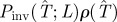. (Online version in colour.)

In the following, we give a general description of the steps for prediction of epidemic invasion with particular assumptions suitable for the analysis of the fungal invasion experiment. The main details of all the methodologies are summarized in table 1. The methodology C is mainly used for illustration of our concepts. Details of other explored methodologies are given in the electronic supplementary material, appendix SI. The motivation for choosing methodology C is twofold: (i) it keeps all the steps for prediction of the behaviour at a similar level of complexity, as illustrated by analysis of the fungal colony invasion in the agar-dot experiment, and (ii) it is a parsimonious methodology that leads to predictions that are, at least, as robust as (or, arguably, even more robust than) those based on more sophisticated approaches (table 1).

Step (i). The information that can be extracted from observation of the time evolution of epidemics is usually limited. In many cases, the only available information is the incidence, C(t) (the number of infected hosts), at subsequent observations, and occasionally the spatial location of infected hosts is also known, e.g. for epidemics in populations of plants [8,22,24,25]. These limitations have a dramatic influence on subsequent steps in the prediction process and it is crucial to identify which quantities are sufficient for prediction of the catastrophic event (i.e. the probability of an invasive epidemic in our case). As shown in table 1, we consider three types of observations. The first consists of discrete temporal observations of C(t) (methods A and B in table 1). The second possibility (methods C–E) considers discrete spatio-temporal observations giving the evolution of infection at discrete times, t, in shells at a ‘chemical distance’ l from the initially inoculated host. As explained in figure 1a, such observations can be properly described in terms of a shell-evolution function F(l,t). As a third possibility (method F), we use a method for data augmentation in step (iii) that infers the unobserved time of infection for each host, {t_i} [8,24,25].

Step (ii). We describe the evolution of the epidemic in terms of a spatial susceptible–infected–removed (SIR) epidemiological model where the hosts can be either susceptible (S), infected (I) or removed (R) [19,21,22,26]. This is a prototype model for a wide class of epidemics where disease leads to permanent immunity of hosts after recovery or death. In particular, this paradigm has been shown to be appropriate for description of fungal invasion [23,27,28]. In principle, a continuous-time dynamic model is necessary to provide a precise description of epidemic evolution characterized by stochasticity in times of infection and removal/recovery of hosts. Following this idea, it would be natural to use a model with continuous-time (CT) dynamics (described in the electronic supplementary material, appendix SI). The drawback of this approach is that it requires knowledge of the precise times of infection of hosts, {t_i}, which are typically not available from discrete spatio-temporal observations in step (i). In order to match an appropriate model with the level of detail of observations, we consider the discrete-time dynamics model that reduces the SIR framework to the so-called Reed–Frost (RF) model [29]. This simplified description is not expected to capture the dynamical details of the evolution of the epidemic, but describes well its final state [30,31]. This is a very important consequence of the fact that, no matter how complicated the evolution of the epidemic is, the final state of an epidemic with death of infected individuals or permanent acquired immunity after recovery depends only on the probability T, called transmissibility, that the infection has ever been passed between each pair of connected hosts (as shown in figure 1b). Although the transmissibility is expected to exhibit a certain degree of spatial heterogeneity in real epidemics, we make the minimal assumption that the trend of the epidemic can be well approximated by an RF process with a homogeneous effective transmissibility T.

Step (iii). The goal of this step is to estimate the values of the parameters of the model used in step (ii) that give a good description of the observations. Consider, for definiteness, methodology C in table 1. Owing to factors such as stochasticity and heterogeneity in transmission, a given observed spatio-temporal map for infection can occur for different values of the estimated transmissibility, T̂. However, some of these values for T̂ are more likely to produce the observed spatio-temporal pattern than others. To account for this, we introduce the probability density function (p.d.f.), ρ(T̂), which quantifies the probability that the observed spatio-temporal pattern is reproduced by a certain value of T̂. As shown schematically in figure 1c, ρ(T̂) is calculated by generating a large number of stochastic realizations of the RF epidemic with transmissibilities T sampled uniformly from the interval [0,1] and comparing their shell-evolution functions, F_sim(l,t) (see caption of figure 1 for definition), with the observed one, F_obs(l,t). Ideally, the distribution ρ(T̂) would correspond to the histogram of values for T̂ producing shell-evolution functions F_sim(l,t) identical to F_obs(l,t) but obtaining an exact match is computationally very demanding. Moreover, reproducing F_obs(l,t) by an RF model is, in general, impossible in realistic epidemics for which time is not discrete. Therefore, we use a minimum distance (MD) algorithm to calculate ρ(T̂) approximately as the histogram of values of T̂ minimizing the quantity d_f² defined in table 1 that measures the distance between F_sim(l,t) and F_obs(l,t). In this way, the sampled values of T̂ reproduce F_obs(l,t) approximately rather than necessarily with distance d_f² = 0. This approach is similar to the approximate Bayesian computation (ABC) method that determines ρ(T̂) as the histogram of values of T̂ for which d_f² ≤ ɛ, where ɛ is a parameter used in the method [32]. Both ABC and MD algorithms give similar results despite the fact that MD does not require the use of an additional parameter ɛ. In addition to these approximate methods, we have fitted the spatio-temporal evolution of the CT model proposed in step (ii) for comparison by means of a more standard Bayesian procedure using Markov chain Monte Carlo (MCMC) method with data augmentation (DA-MCMC) (method F in table 1).

Step (iv). In the final stage of the prediction process, given ρ(T̂), we evaluate the probability that the observed epidemic will ever invade a system of size L. The epidemic is defined as being invasive if the final cluster of removed hosts has reached at least one node on each of the six edges of the system. Otherwise, the epidemic is classified as being non-invasive. The conditional probability of invasion P_inv(T̂;L) in a system of size L by an SIR process with a given transmissibility, T̂, can be calculated numerically by running many stochastic realizations of the epidemic and counting the fraction of invading events. As shown in figure 1d, P_inv(T̂;L) exhibits a sigmoidal dependence on T̂ which indicates a non-invasive (invasive) regime of epidemics for relatively small (large) values of T̂. Once P_inv(T̂;L) and ρ(T̂) are known, the estimated probability of invasion can be calculated as follows:

2.1

This formula defines the probability that the invasion occurs given our knowledge about the effective transmissibility encoded by ρ(T̂) (see a simple graphical interpretation in terms of the shaded area in figure 1d). Importantly, equation (2.1) gives an extrapolation of the behaviour of the epidemic to its final state without necessarily providing a detailed description of the actual evolution leading to such a state.

3. Application to fungal invasion

In the fungal invasion experiments, the spatio-temporal maps of infected agar dots were scored daily over 21 days (see two typical patches of colonization after 21 days in figure 2a). The transmissibility in this experiment corresponds to the probability of fungal colonization between two adjacent agar dots and it was controlled by variable lattice spacing, a = 8, 10, 12, 14, 16, 18 mm. Clearly, the experimental set-up is restricted both in space and time. Our aim is to use these limited observations to estimate the probability of invasive epidemics in larger systems and for longer times. The analysis is performed for each individual realization of the experiment (six replicates per value of a).

Figure 2.

Fungal invasion in the system of agar dots placed on a triangular lattice. (a) The observed mean probability of invasion P_exp obtained by counting the relative number of invasive epidemics after 21 days is shown by the solid line. The probability of invasion after 21 days was estimated for each replicate by observing the initial evolution of colonization during t_obs = 10 days. The corresponding mean over replicates with the same value of a is shown with a different symbol type (the same as in figures 4 and 5) for each method for prediction. The inserts show the invasive (left) and non-invasive (right) state of the epidemic after 21 days for two representative replicates with lattice spacings a = 10 mm and a = 14 mm, as marked by arrows. Solid (open) circles in the inserts represent colonized (not colonized) dots. (b) Prediction of with different methodologies for individual replicates of the epidemic in a large system of size L = 51 obtained from observations during t_obs = 21 days of the smaller experimental system (L < 8). The mean of over replicates for each value of a is shown by different symbol types corresponding to different methodologies. The mean probability of invasion P_exp obtained by counting the relative number of invasive epidemics after 21 days is shown by the solid line. (Online version in colour.)

In order to make a proper comparison between the experimental observations with the RF model used in methods A–D, it is necessary to rescale the time step of the RF dynamics with dimensionless τ = 1 to measured in days. The value of is not known and it is treated at the same level as the transmissibility. More explicitly, we deal with a bi-variate p.d.f., , which can be determined for each epidemic with a simple extension of the methods explained in §2 (step (iii)) for obtaining ρ(T̂). The estimated is obtained from equation (2.1) by defining ρ(T̂) as the marginal p.d.f., . As explained in more detail in the electronic supplementary material, §I of appendix SI and summarized in table 1, the continuous-time SIR model used in methods E and F involves three parameters: T, τ₀ and k. The fitting of the data results in a p.d.f. ρ₃(T, τ₀, k) from which we obtain . The probability of invasion is then calculated from equation (2.1) in the same way as for methods A–D.

3.1. Uncertainty of the estimated transmissibility

The functions ρ(T̂) obtained for the fungal invasion experiments typically exhibit a pronounced peak (see the results for one replicate in figure 3 and similar results for more replicates in the electronic supplementary material, figure S1 of appendix SI). The peaked shape of ρ(T̂) suggests that T̂ can be suitably described in terms of its mean value 〈T̂〉 and standard deviation . For each methodology, figure 4 shows the average over replicates of 〈T̂〉 and σ_T as a function of the lattice spacing. These estimates correspond to observations of the evolution of infection during t_obs = 21 days. All the methods give similar values for 〈T̂〉 which have a clear and expected tendency to decrease with increasing a. The uncertainty in T̂, quantified by σ_T, exhibits greater variations between methodologies but it takes values that are smaller than 〈T̂〉 for all the methods and lattice spacings (figure 4b). This means that 〈T̂〉 is a good measure of the typical value of the transmissibility. However, the value of 〈T̂〉 on its own does not necessarily provide a good approximation for because the width of ρ(T̂) can bring a significant contribution to the integral in equation (2.1). This is explicitly shown in §4.

Figure 3.

Estimates of the transmissibility for fungal invasion in the system of agar dots. The p.d.f.'s ρ(T̂) obtained with different fitting methodologies are plotted for the fungal colony invasion in a population of agar dots with lattice spacing a = 10 mm. Estimates correspond to observation of the fungal spread during t_obs = 21 days. Different symbol types correspond to different fitting methodologies, as marked in the legend. Electronic supplementary material, figure S1 in appendix SI shows similar plots for six replicates of the system. (Online version in colour.)

Figure 4.

Statistical characteristics of the estimates of the transmissibility for fungal invasion in the system of agar dots. Dependence on the lattice spacing of (a) the mean value 〈T̂〉, and (b) standard deviation σ_T of the transmissibility calculated from the p.d.f. ρ(T̂) corresponding to observations during t_obs = 21 days. For clarity, each symbol gives the average of (a) 〈T̂〉 and (b) σ_T over six replicates of the experiments for each lattice spacing, a. As marked in the legend, different symbol types correspond to different methods for addressing the steps (i)–(iii) summarized in table 1. (Online version in colour.)

Comparison of 〈T̂〉, σ_T and ρ(T̂) for different methods leads to the following conclusions.

• — Given a level of description (step (i)) and a model (step (ii)), the estimates of the transmissibility obtained with ABC and MD methods are, in general, in good agreement (cf. method A with method B, and method C with method D in figures 3 and 4).

• — Given a level of description (step (i)) and an estimation method (step (iii)), the posteriors obtained using discrete- and continuous-time models are in reasonable agreement (cf. method D with method E in figures 3 and 4). The only difference is a trend for ρ(T̂) corresponding to CT dynamics to have a ‘heavy tail’ for large values of T̂ (see the replicate 4 in the electronic supplementary material, figure S1, appendix SI). Large values of T̂ are correlated with large values of the time scale τ₀ (i.e. slower processes with high T̂) and small values of the shape parameter k, that are ruled out by the RF model. This effect becomes more important for larger values of the lattice spacing, as indicated by the large values of 〈T〉 and σ_T corresponding to Method E (asterisks in figure 4).

• — The estimates from DA-MCMC (methodology F) are, in general, different from those obtained by other methods. Moreover, the p.d.f.'s ρ(T̂) obtained with MCMC show no systematic trend with respect to the other methods. With respect to, e.g. the ρ(T̂) obtained with MD, they can be located at slightly higher (replicates 5 and 6 in the electronic supplementary method, figure S1) or lower (replicates 2 and 3) values of T̂, or approximately at the same value (replicates 1 and 4). Moreover, the variation in the peak position of ρ(T̂) between different replicates is larger than for the other methods. This suggests that the MCMC method is more sensitive to fine details of the evolution of the epidemic. A possible explanation is that DA-MCMC involves the inference of the unobserved colonization times and thus is intrinsically individual-based, in contrast to shell-based (or mean-field) methods, which try to match the colonization times in an approximate manner only.

3.2. Comparison of fitted models with experimental data

In order to assess the quality of the assumptions used for estimation, we compare the fitted models with the available experimental data. For methods A–D, we compare the incidence and shell-evolution function obtained numerically (RF dynamics) with values for T̂ and sampled from estimated by means of the spatio-temporal maps at maximum observation time t_obs = 21 days with the actual incidence and shell-evolution function for each epidemic. Similarly, the fits from methods E and F are compared with experimental observations by running numerical epidemics with parameters for the CT dynamics sampled from the p.d.f. ρ₃ (T̂, τ₀, k). We make a quantitative comparison based on squared distances d_c² and d_f² (cf. table 1) between simulated epidemics and experimental fungal invasions. More explicitly, we define the root mean square (r.m.s.) distances,

3.1

and

3.2

where Δt = 21 days is the time interval used for calculations of d_c² or d_f². The quantity l_max is the maximum chemical distance to the centre of the system of agar dots. Its value decreases with the lattice spacing and ranges from l_max = 2 for a = 16 mm to l_max = 8 for a = 8 mm [23]. From the definition of d_c² given in table 1, it is easy to see that Δc gives the typical deviation of the simulated incidence per unit host at a given time, c_sim(t), from the observed incidence per host at the same time, c_obs(t). Similarly, ΔF gives the typical deviation of the simulated shell-evolution function, F_sim, evaluated at any spatio-temporal coordinates (l,t) from the observed value at the same coordinates.

Figure 5 shows the mean of the r.m.s. distances obtained by averaging over stochastic simulations and over replicates with given lattice spacing. The low values of the r.m.s. distances (Δc ≲ 0.2 and ΔF ≲ 0.3) indicate that the observed C(t) and F(l,t) are statistically well described by the fitted models. For any given method and lattice spacing, we obtained Δc < ΔF, which is expected because reproducing the spatio-temporal evolution represented by F(l,t) is more demanding than capturing the temporal evolution of the colonization given by c(t). Both Δc and Δ F tend to be larger for a around 10–12 mm which, as shown below, corresponds to cases that are close to the invasion threshold (i.e. where P_inv decreases from 1 to 0 on increasing a as shown by the solid line in figure 2a). Variability between replicates of epidemics with given T is larger around the invasion threshold, which is associated with a critical phase transition and characterized by large fluctuations [13,21,23,26–28]. As a consequence, the quality of fits is lower in the vicinity of the invasion threshold and this leads to larger values of Δc and ΔF.

Figure 5.

Comparison of fitted models with experimental data. Mean root mean square (r.m.s.) distances (a) Δc and (b) ΔF between observed and simulated fungal invasions in populations of agar dots. The mean value of r.m.s. distances is obtained by averaging over 10⁴ stochastic realizations of simulations and over six replicates for each lattice spacing, a. Simulations are based on fits to observations over t_obs = 21 days. Different symbols correspond to different methodologies summarized in table 1, as marked in the legend. (Online version in colour.)

Methodology C gives a good balance between performance and number of parameters involved. Methods C–E based on an approximate spatio-temporal description of epidemics given by F(l,t) result in more accurate predictions than methods A (squares in figure 5) and B (diamonds) that neglect spatial features of invasion. Moreover, the approximate methods C–E also perform better than even methodology F (triangles in figure 5), despite the fact that the latter aims for a more precise spatio-temporal description. A more qualitative and visual comparison of estimated and observed C(t) reveals similar differences between all the methodologies (see details in the electronic supplementary material, §III of appendix SI).

3.3. Two applications for prediction methods

As a first application of the proposed methods, we have studied the predictive power of the estimates of the probability of invasion and the incidence by calculating ρ(T̂) from the early stages of the actual epidemic, i.e. for t_obs < 21 days. In particular, based on the estimated ρ(T̂) for t_obs = 10 days, we have obtained estimates for the probability of invasion at time t = 21 days and compared them with the probability P_exp of invasion at t = 21 days obtained directly from the experimental data. The observed probability of invasion, P_exp, is estimated by counting (for each a) the fraction of replicates in which the fungus has reached the six outer edges of the experimental system by 21 days. The mean of averaged over replicates with the same value of a (symbols in figure 2a) gives a reasonable estimate for the observed mean of P_exp (solid curve in figure 2a) after t = 21 days for most of the methods. Overall, the best predictions for are obtained with methodology C (solid circles in figure 2a). As expected, decreases with increasing a for all methodologies, illustrating the existence of the threshold for epidemics around a ≃ 12 mm [23]. Similarly, the experimentally observed incidence and shell-evolution function are statistically well captured by the numerical extrapolation for their simulated counterparts up to time t = 21 days obtained from observations over times t_obs < 21 days. A visual illustration of the agreement between the observed and predicted incidence is given in the electronic supplementary material, §IV of appendix SI. Figure 6 shows the r.m.s. distances between the observed and predicted evolutions from day 11 to day 21. The time interval used to calculate Δc and ΔF from equations (3.1) and (3.2) is Δt = 11 days. The relative trends of Δc and ΔF between methods and lattice spacings are similar to those reported in figure 5 for the comparison between observations and numerical simulations with t_obs. The main difference is that the values of the r.m.s. distances corresponding to predictions of the evolution of colonization (figure 6) are systematically larger than those obtained by simply comparing observed evolutions with their respective fittings (figure 5). This is in agreement with the intuitive idea that predicting the a priori unknown evolution of a system is more challenging than reproducing a fitted evolution.

Figure 6.

Comparison of the predicted and observed evolution of fungal invasion in the system of agar dots. Predictions of the fungal spread in the period of time between days 10 and 21 are made from observation of the initial spread during t_obs = 10 days. The vertical axes show the mean over replicates of the r.m.s. distances (a) Δc and (b) ΔF between observed and predicted fungal evolution during the time interval 11−21 days. The mean value of r.m.s. distances is obtained by averaging over stochastic realizations of simulations and over six replicates for each lattice spacing, . Simulations are based on fittings to observations over t_obs = 10 days. Different symbols correspond to different methodologies summarized in table 1, as marked in the legend. (Online version in colour.)

As a second application of our methodology, we have calculated at the end of the epidemic as a function of the lattice spacing in systems of size L = 51, i.e. larger than the experimental samples of sizes L = 2, … 8, which decrease with increasing lattice spacing (see the two populations for different values of a shown in figure 2a). Such predictions are based on estimates for the transmissibility obtained from observations up to t_obs = 21 days. As expected, decreases with increasing a. The results of applying each of the prediction methods are shown in figure 2b for the mean probability averaged over replicates for each value of a. All the methods except E give similar predictions for . The large values of predicted by method E are a consequence of the ‘heavy tail’ of the p.d.f. ρ(T̂), which gives a significant weight to the high values of P_inv for large T̂ in equation (2.1). The dependence of on a differs from the observed probability of invasion, P_exp (solid curve in figure 2b). The difference can be qualitatively understood by recalling that gives an extrapolation both in space and time. Indeed, because some epidemics that are non-invasive after 21 days have a certain probability to invade a system of size L = 51 for t > 21 days. In addition, both infectivity and susceptibility are expected to be subject to heterogeneity in the agar-dot system owing to, e.g. inherent variability. Based on the results presented in §4 for numerical experiments with heterogeneity in transmission, we expect the estimated to give an upper bound to the actual probability of invasion. This can also contribute to the difference between and P_exp for large values of a.

4. Numerical experiment

The quality of the predictions presented in §3 is influenced by the quality of the observations in step (i), the suitability of the model chosen in step (ii) for description of the data, and the fitting procedure used in step (iii). In principle, the effect of these factors on predictions could be minimized by optimizing the procedures used in each step for prediction. Stochasticity associated with the transmission of infection also influences the ability of making reliable predictions. In contrast to the previous factors, stochasticity is inherent to the nature of the system and its negative effect on predictions cannot be minimized without modifying the system. In this section, we present a sensitivity analysis of our methods by applying them to prediction of invasion for numerically simulated epidemics, where the main factor compromising predictability is the intrinsic stochasticity in transmission of infection. The advantage in this case with respect to more realistic situations is that both the transmissibility, T, and the probability of invasion, P_inv(T;L), are known and it is then possible to investigate the performance of the estimates for ρ(T̂) and by comparing with the known quantities.

We first consider the simplest situation when the observed epidemics follow the RF dynamics with homogeneous transmission (i.e. T is the same for all pairs of nearest neighbours in the population). The idea is to run numerical experiments with known T, observe the evolution of the epidemic over an initial interval of time, t_obs, and then apply the methods described above to calculate assuming that T is unknown (as it occurs for real epidemics).

For concreteness, we consider the arrangement shown in figure 1a and use methodology C for steps (i)–(iii). RF epidemics are observed during t_obs = 7τ with the aim of estimating the probability that they will invade a system of size L = 51. Note that over the time interval t ≤ t_obs = 7, the epidemic at most invades a hexagon of size L = 15. Then, the behaviour of the epidemic is extrapolated both in space and time. We proceed by, first, calculating the p.d.f. ρ(T̂) for the estimated transmissibilities T̂ compatible with observation (spatio-temporal map). Figure 1c shows an example of ρ(T̂) obtained from the analysis of the evolution of an epidemic with T = 0.4. In general, the most probable estimate for the transmissibility, , corresponding to the maximum of ρ(T̂) for a single epidemic, differs from T but not significantly. In many cases, T lies within the 68 per cent confidence interval for ρ(T̂) around its maximum (see a more detailed discussion in the electronic supplementary material, appendix SI). The distribution ρ(T̂) allows the probability of invasion in the system of size L = 51 to be estimated using equation (2.1). We have applied this prediction method to many (∼10⁴) spatio-temporal maps created with known transmissibility T spanning the interval [0,1]. For each value of estimated , the distribution ρ(T̂) is represented by a horizontal slice of the shaded area in figure 7 (see the slice along the dashed blue line corresponding to with darker colour corresponding to higher probability relative to the maximum of ρ(T̂)). The black ridge in the shaded area corresponds to the most probable transmissibility, , for each value of .

Figure 7.

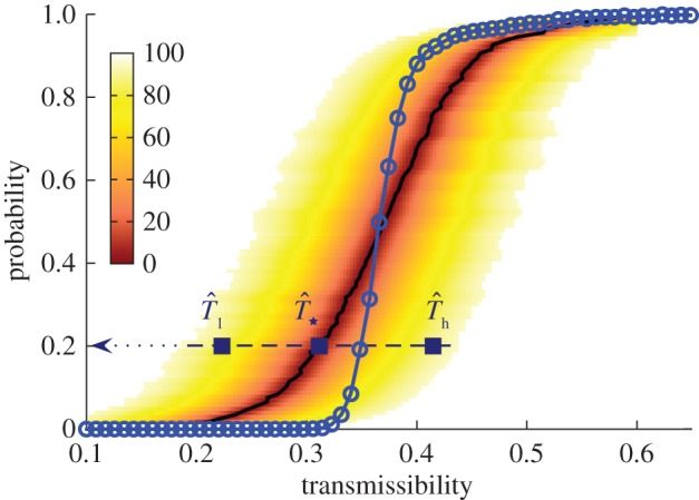
Numerical experiments of SIR epidemics with homogeneous transmissibility. Hosts are placed on the nodes of a triangular lattice of size L = 51 (cf. figure 1a). The evolution of epidemics starting from the central host is observed over time t ≤ t_obs = 7τ. The line marked by circles shows the dependence of the conditional probability of invasion, P_inv(T;L), on transmissibility obtained by the simulations in the system of size L = 51. The shaded region shows the levels of confidence in percentage of the p.d.f ρ(T̂) around the most probable transmissibility, (solid black line) corresponding to each value of . The horizontal dashed line illustrates the case of estimations giving . If the observed epidemic has a value of the transmissibility such as that is to the left of the curve for P_inv (line with circles), the estimated overestimates P_inv. By contrast, for values of the transmissibility that are to the right of the curve for P_inv (e.g. ), the probability underestimates P_inv. (Online version in colour.)

To test the quality of the predictions, the estimate of the probability of invasion P_inv(T̂;L) is compared with the probability P_inv(T;L) that would be obtained if the exact value of T was known a priori (see line marked by circles in figure 7). Making such a comparison we can see that for epidemics with low transmissibility where invasion is possible but not highly probable, overestimates P_inv(T;L) for most of the possible values of T̂ contributing to (the shaded area including the ridge region corresponding to the typical values of T̂ is mainly above the line marked by circles in figure 7). This means that the estimations are biased upwards and most likely is that the actual probability of invasion will be smaller than predicted. In other words, such predictions will typically give a safe bound for the probability of invasion. Obviously, there is a non-zero probability that the observed epidemic has a large value of the transmissibility (such as in figure 7). In this case, would underestimate the actual probability P_inv. For more invasive epidemics (i.e. epidemics with P_inv∼0.5), the shaded area is mainly below the line marked by the circles in figure 7 meaning that the predicted probability of invasion underestimates P_inv for most of the possible values for T̂, including the most probable, . In these situations however, both and P_inv are large and the predictions allow for a reasonable assessment for invasion to be done. In the electronic supplementary material, §VI of appendix SI, we show mathematically that differences between and P_inv evaluated at the most probable transmissibility are mainly dictated by the curvature of P_inv around and is intrinsically linked to the non-zero width of the p.d.f. ρ(T̂). This general result implies that the biases in the probability of invasion at low and high transmissibility are independent of the fitting method (table 1) because all methods lead to a p.d.f. ρ(T̂) with non-zero width.

The results presented above correspond to RF epidemics with homogeneous transmission. A similar approach has been used to deal with more realistic epidemics where the transmission of infection is heterogeneous owing to variability in the infectivity and the susceptibility of hosts. As already mentioned in §3, the estimated for such epidemics usually gives a bound to the actual probability of invasion that is even safer than that obtained for cases with homogeneous transmissibility (see the electronic supplementary material, §V.B, appendix SI for more detail).

5. Discussion

The methodology introduced here focuses on the prediction of relatively simple but important features of epidemics. This is in contrast to much previous work dealing with the prediction of quantitative properties of epidemics such as the detailed spatio-temporal evolution of the incidence. The advantage in dealing with simple characteristics of epidemics is that they can be more easily predicted in terms of simplified description of the spatio-temporal evolution. Our results demonstrate that, under quite general assumptions, it is possible to give reliable prediction of the final state of an epidemic with permanent immunization from the early stage of its evolution. Such a prediction is possible even for a single realization of an epidemic and thus the framework is relevant to inherently unique real-world epidemics. In fact, our approach can be applied for prediction of epidemics in real systems characterized by a wide range of space and time scales (e.g. crops) based on micro- or meso-cosm experiments of finite size and over finite time.

The results obtained for experimental fungal invasion by using approximate methods (C–E in table 1) are more robust than those based on supposedly more precise methodology F. This might be a consequence of the interplay between the high-fitting precision for MCMC methods involving data augmentation with a poor description of the actual dynamics given by the continuous-time model fitted to the observations. A model capturing dynamical details at a level consistent with that offered by the fitting procedure might exhibit more predictive power than that presented here. This is an illustration of the importance of keeping all the steps involved in prediction at a similar level of complexity in order to give reliable predictions. For practical applications, the particular method to be used for obtaining the most reliable prediction depends on the problem in hand. The general rule that seems to emerge from our analysis is that a reasonable method should use as much information as available from observations, and avoid inferring data that are not directly available unless it is strictly required by the problem. This is the case for methods C–E in our particular study of fungal colony invasion in the population of agar dots. Methods A and B use less information than available from observations (i.e. they use C(t) instead of F(l,t)), while method F infers information that is not available from observations.

The proposed methods assume that epidemics can be approximately described by an effective transmissibility that is constant over time and homogeneous in space. However, their applicability goes beyond epidemics with constant transmissibility. In particular, we have shown that the method gives reliable predictions in the presence of spatial heterogeneity in the transmission of infection. We expect that the methodology can also be successfully applied to cases where the transmissibility changes over time but it remains within the bounds for the effective transmissibility estimated from the early stage.

We have characterized the final state of epidemics by the probability of invasion. This quantity is suitable for systems with well-defined boundaries such as the population of agar dots analysed above. In cases where hosts are placed on the nodes of more complex networks, the boundaries of the system are not necessarily well-defined [33] and it is more convenient to characterize the final state of epidemics in terms of the mean number of removed (i.e. ever infected) hosts, N_R. Our approach also applies to such complex networks. The formula given by equation (2.1) provides an estimated size, , if P_inv(T̂;L) is replaced by the function N_R(T̂;L) giving the size of SIR epidemics with given transmissibility, T̂.

Our methods have been applied under the assumption that the network of contacts between hosts remains unchanged during the course of epidemics. Such an approximation has been widely used in the past [33] and it is reasonable for cases in which the rate of change of the configuration of contacts is much smaller than the removal rate of hosts (i.e. ∼τ⁻¹ in our notation). This condition is clearly satisfied for the fungal colony invasion of the population of agar dots considered here and also for many other epidemics associated with pathogens spreading in, e.g. networks of plants [22], farms [9] or airports [11]. This paradigm is also applicable to the spread of many infections in human populations (for instance, measles or severe acute respiratory syndrome that have recovery periods of the order of few days). By contrast, the dynamics of contacts between humans plays an important role for other infectious diseases such as syphilis with a recovery period of 100 days [34]. A possible strategy to make predictions in this kind of networks would involve inferring the mixing parameter for contacts (as defined, for instance, in Volz & Meyers [34]) based on observations (step (i)) in a similar way as we estimated the parameters of the SIR model in step (iii).

Another interesting task would be to extend the ideas presented here to deal with epidemics with persistence where immunity after recovery is not permanent (i.e. recovered hosts can be re-infected). In this case, the simplest model for description of observations is the susceptible–infected–susceptible model [35] and a possible quantity to be predicted would be the stationary prevalence of infection (i.e. the density of infected hosts in the stationary state reached after a transient [35]).

Owing to stochasticity in transmission of infection, it is not possible to determine the parameters of a model describing an epidemic with absolute certainty even if the epidemic is observed during a long time t_obs before attempting inference. Furthermore, if it were possible to determine the exact value of the parameters, it would still be impossible to make arbitrarily precise predictions of the evolution of the epidemic in the future or predict with absolute certainty if the epidemic is going to be invasive or not (instead, one has to deal with the probability of invasion). The uncertainty in the prediction of the evolution of epidemics grows monotonically with the look-ahead time (see the forecast of the incidence in the electronic supplementary material, §IV of appendix SI). There exists a prediction horizon beyond which the uncertainty of predictions of the evolution of the epidemic is too large for predictions to be useful. The location of the horizon is epidemic-dependent and also depends on how precise we want our predictions to be. By contrast, for a pure SIR epidemic, there is no prediction horizon for quantities such as P_inv or N_R that only depend on the transmissibility. In other words, different replicates of epidemics with given T will follow different evolutions that have a prediction horizon but will lead to the same P_inv or N_R [26,30,31]. More complex nonlinear dynamics for transmission associated with, for instance, a seasonal component in the transmission rate may lead to chaotic behaviour [36]. Predictability of catastrophic events in systems exhibiting chaotic behaviour is a non-trivial question that has been widely studied in the past [37] and still receives considerable attention presently [38]. Even in the absence of stochasticity, the prediction horizon in these systems is intrinsically limited owing to the high sensitivity of chaotic processes to the initial conditions and the values of the parameters. In addition, the accuracy of predictions does not necessarily increase monotonically with the observation time, t_obs, before prediction [39]. In such situations, it would be necessary to estimate the value of t_obs leading to the most reliable prediction. Owing to all these factors, the methods proposed in this paper may not work when applied for prediction of catastrophic events in nonlinear dynamical systems. However, the ideas presented here together with approaches proposed for prediction in nonlinear dynamical systems may help in devising strategies for prediction in stochastic nonlinear systems.

References

- 1.Sornette D. 2000. Critical phenomena in natural sciences. Springer Series in Synergetics Berlin, Germany: Springer [Google Scholar]
- 2.Sornette D. 2002. Predictability of catastrophic events: material rupture, earthquakes, turbulence, financial crashes, and human birth. Proc. Natl Acad. Sci. USA 99, 2522–2529 10.1073/pnas.022581999 (doi:10.1073/pnas.022581999) [DOI] [PMC free article] [PubMed] [Google Scholar]
- 3.Sornette D. 2003. Why stock markets crash. Princeton, NJ: Princeton University Press [Google Scholar]
- 4.Medley G. F. 2001. EPIDEMIOLOGY: predicting the unpredictable. Science 294, 1663–1664 10.1126/science.1067669 (doi:10.1126/science.1067669) [DOI] [PubMed] [Google Scholar]
- 5.Valleron A. J., Boelle P. Y., Will R., Cesbron J. Y. 2001. Estimation of epidemic size and incubation time based on age characteristics of vCJD in the United Kingdom. Science 294, 1726–1728 10.1126/science.1066838 (doi:10.1126/science.1066838) [DOI] [PubMed] [Google Scholar]
- 6.d'Aignaux J. N. H., Cousens S. N., Smith P. G. 2001. Predictability of the UK variant Creutzfeldt–Jakob disease epidemic. Science 294, 1729–1731 [DOI] [PubMed] [Google Scholar]
- 7.Morton A., Finkenstädt B. F. 2005. Discrete time modelling of disease incidence time series by using Markov chain Monte Carlo methods. J. R. Stat. Soc. C 54, 575–594 [Google Scholar]
- 8.Kleczkowski A., Gilligan C. 2007. Parameter estimation and prediction for the course of a single epidemic outbreak of a plant disease. J. R. Soc. Interface 4, 865–877 10.1098/rsif.2007.1036 (doi:10.1098/rsif.2007.1036) [DOI] [PMC free article] [PubMed] [Google Scholar]
- 9.Keeling M. J., et al. 2001. Dynamics of the 2001 UK foot and mouth epidemic: stochastic dispersal in a heterogeneous landscape. Science 294, 813–817 10.1126/science.1065973 (doi:10.1126/science.1065973) [DOI] [PubMed] [Google Scholar]
- 10.Ferguson N. M., Donnelly C. A., Anderson R. M. 2001. The foot-and-mouth epidemic in Great Britain: pattern of spread and impact of interventions. Science 292, 1155–1160 10.1126/science.1061020 (doi:10.1126/science.1061020) [DOI] [PubMed] [Google Scholar]
- 11.Hufnagel L., Brockmann D., Geisel T. 2004. Forecast and control of epidemics in a globalized world. Proc. Natl Acad. Sci. USA 101, 15 124–15 129. 10.1073/pnas.0308344101 (doi:10.1073/pnas.0308344101) [DOI] [PMC free article] [PubMed] [Google Scholar]
- 12.Riley S. 2007. Large-scale spatial-transmission models of infectious disease. Science 316, 1298–1301 10.1126/science.1134695 (doi:10.1126/science.1134695) [DOI] [PubMed] [Google Scholar]
- 13.Pérez-Reche F. J., Taraskin S. N., Costa L.D.A.F., Neri F. M., Gilligan C. A. 2010. Complexity and anisotropy in host morphology make populations less susceptible to epidemic outbreaks. J. R. Soc. Interface 7, 1083–1092 10.1098/rsif.2009.0475 (doi:10.1098/rsif.2009.0475) [DOI] [PMC free article] [PubMed] [Google Scholar]
- 14.Truscott J. E., Gilligan C. A. 2003. Response of a deterministic epidemiological system to a stochastically varying environment. Proc. Natl Acad. Sci. USA 100, 9067–9072 10.1073/pnas.1436273100 (doi:10.1073/pnas.1436273100) [DOI] [PMC free article] [PubMed] [Google Scholar]
- 15.Dye C., Gay N. 2003. EPIDEMIOLOGY: modeling the SARS epidemic. Science 300, 1884–1885 10.1126/science.1086925 (doi:10.1126/science.1086925) [DOI] [PubMed] [Google Scholar]
- 16.May R. M. 2004. Uses and abuses of mathematics in biology. Science 303, 790–793 10.1126/science.1094442 (doi:10.1126/science.1094442) [DOI] [PubMed] [Google Scholar]
- 17.Pearce N., Merletti F. 2006. Complexity, simplicity, and epidemiology. Int. J. Epidemiol. 35, 515–519 10.1093/ije/dyi322 (doi:10.1093/ije/dyi322) [DOI] [PubMed] [Google Scholar]
- 18.Goldenfeld N., Kadanoff L. P. 1999. Simple lessons from complexity. Science 284, 87–89 10.1126/science.284.5411.87 (doi:10.1126/science.284.5411.87) [DOI] [PubMed] [Google Scholar]
- 19.Anderson R. M., May R. M. 1991. Infectious diseases of humans: dynamics and control. Oxford, UK: Oxford University Press [Google Scholar]
- 20.Murray J. D. 2002. Mathematical biology. I. An introduction, 3rd edn. Berlin, Germany: Springer [Google Scholar]
- 21.Davis S., Trapman P., Leirs H., Begon M., Heesterbeek J. 2008. The abundance threshold for plague as a critical percolation phenomenon. Nature 454, 634– 637 10.1038/nature07053 (doi:10.1038/nature07053) [DOI] [PubMed] [Google Scholar]
- 22.Otten W., Filipe J. A. N., Bailey D. J., Gilligan C. A. 2003. Quantification and analysis of transmission rates for soilborne epidemics. Ecology 84, 3232–3239 10.1890/02-0564 (doi:10.1890/02-0564) [DOI] [Google Scholar]
- 23.Bailey D. J., Otten W., Gilligan C. A. 2000. Saprotrophic invasion by the soil-borne fungal plant pathogen Rhizoctonia solani and percolation thresholds. New Phytol. 146, 535–544 10.1046/j.1469-8137.2000.00660.x (doi:10.1046/j.1469-8137.2000.00660.x) [DOI] [Google Scholar]
- 24.Gibson G. J., Kleczkowski A., Gilligan C. A. 2004. Bayesian analysis of botanical epidemics using stochastic compartmental models. Proc. Natl Acad. Sci. USA 101, 12 120–12 124. 10.1073/pnas.0400829101 (doi:10.1073/pnas.0400829101) [DOI] [PMC free article] [PubMed] [Google Scholar]
- 25.Gibson G. J., et al. 2006. Bayesian estimation for percolation models of disease spread in plant populations. Stat. Comput. 16, 391–402 10.1007/s11222-006-0019-z (doi:10.1007/s11222-006-0019-z) [DOI] [Google Scholar]
- 26.Grassberger P. 1983. On the critical behavior of the general epidemic process and dynamical percolation. Math. Biosci. 63, 157–172 10.1016/0025-5564(82)90036-0 (doi:10.1016/0025-5564(82)90036-0) [DOI] [Google Scholar]
- 27.Otten W., Bailey D. J., Gilligan C. A. 2004. Empirical evidence of spatial thresholds to control invasion of fungal parasites and saprothophs. New Phytol. 163, 125–132 10.1111/j.1469-8137.2004.01086.x (doi:10.1111/j.1469-8137.2004.01086.x) [DOI] [PubMed] [Google Scholar]
- 28.Neri F., et al. 2011. The effect of heterogeneity on invasion in spatial epidemics: from theory to experimental evidence in a model system. PLoS Comput. Biol. 7, e1002174. 10.1371/journal.pcbi.1002174 (doi:10.1371/journal.pcbi.1002174) [DOI] [PMC free article] [PubMed] [Google Scholar]
- 29.Daley D. J., Gani J. 1999. Epidemic modelling. Cambridge, UK: Cambridge University Press [Google Scholar]
- 30.Ludwig D. 1975. Final size distribution for epidemics. Math. Biosci. 23, 33–46 10.1016/0025-5564(75)90119-4 (doi:10.1016/0025-5564(75)90119-4) [DOI] [Google Scholar]
- 31.Pellis L., Ferguson N. M., Fraser C. 2008. The relationship between real-time and discrete-generation models of epidemic spread. Math. Biosci. 216, 63–70 10.1016/j.mbs.2008.08.009 (doi:10.1016/j.mbs.2008.08.009) [DOI] [PubMed] [Google Scholar]
- 32.Marjoram P., Molitor J., Plagnol V., Tavaré S. 2003. Markov chain Monte Carlo without likelihoods. Proc. Natl Acad. Sci. USA 100, 15 324–15 328. 10.1073/pnas.0306899100 (doi:10.1073/pnas.0306899100) [DOI] [PMC free article] [PubMed] [Google Scholar]
- 33.Barrat A., Barthélemy M., Vespignani A. 2008. Dynamical processes on complex networks. Cambridge, UK: Cambridge University Press [Google Scholar]
- 34.Volz E., Meyers L. A. 2007. Susceptible–infected–recovered epidemics in dynamic contact networks. Proc. R. Soc. B 274, 2925–2934 10.1098/rspb.2007.1159 (doi:10.1098/rspb.2007.1159) [DOI] [PMC free article] [PubMed] [Google Scholar]
- 35.Marro J., Dickman R. 1999. Nonequilibrium phase transitions in lattice models. Cambridge, UK: Cambridge University Press [Google Scholar]
- 36.Olsen L., Schaffer W. 1990. Chaos versus noisy periodicity: alternative hypotheses for childhood epidemics. Science 249, 499–504 10.1126/science.2382131 (doi:10.1126/science.2382131) [DOI] [PubMed] [Google Scholar]
- 37.Abarbanel H. D. I., Brown R., Sidorowich J. J., Tsimring L. S. 1993. The analysis of observed chaotic data in physical systems. Rev. Mod. Phys. 65, 1331–1392 10.1103/RevModPhys.65.1331 (doi:10.1103/RevModPhys.65.1331) [DOI] [Google Scholar]
- 38.Wang W. X., Yang R., Lai Y. C., Kovanis V., Grebogi C. 2011. Predicting catastrophes in nonlinear dynamical systems by compressive sensing. Phys. Rev. Lett. 106, 154101. 10.1103/PhysRevLett.106.154101 (doi:10.1103/PhysRevLett.106.154101) [DOI] [PMC free article] [PubMed] [Google Scholar]
- 39.Van Dyke Parunak H., Belding T., Brueckner S. 2008. Prediction horizons in agent models. In Engineering environment-mediated multi-agent systems (eds Weyns D., Brueckner S., Demazeau Y.), lecture notes in computer science, no. 5049, pp. 88–102 Berlin, Germany: Springer. [Google Scholar]