Sexual dimorphism in multiple aspects of 3D facial symmetry and asymmetry defined by spatially dense geometric morphometrics

Abstract

Accurate measurement of facial sexual dimorphism is useful to understanding facial anatomy and specifically how faces influence, and have been influenced by, sexual selection. An important facial aspect is the display of bilateral symmetry, invoking the need to investigate aspects of symmetry and asymmetry separately when examining facial shape. Previous studies typically employed landmarks that provided only a sparse facial representation, where different landmark choices could lead to contrasting outcomes. Furthermore, sexual dimorphism is only tested as a difference of sample means, which is statistically the same as a difference in population location only. Within the framework of geometric morphometrics, we partition facial shape, represented in a spatially dense way, into patterns of symmetry and asymmetry, following a two-factor anova design. Subsequently, we investigate sexual dimorphism in symmetry and asymmetry patterns separately, and on multiple aspects, by examining (i) population location differences as well as differences in population variance-covariance; (ii) scale; and (iii) orientation. One important challenge in this approach is the proportionally high number of variables to observations necessitating the implementation of permutational and computationally feasible statistics. In a sample of gender-matched young adults (18–25 years) with self-reported European ancestry, we found greater variation in male faces than in women for all measurements. Statistically significant sexual dimorphism was found for the aspect of location in both symmetry and asymmetry (directional asymmetry), for the aspect of scale only in asymmetry (magnitude of fluctuating asymmetry) and, in contrast, for the aspect of orientation only in symmetry. Interesting interplays with hypotheses in evolutionary and developmental biology were observed, such as the selective nature of the force underpinning sexual dimorphism and the genetic independence of the structural patterns of fluctuating asymmetry. Additionally, insights into growth patterns of the soft tissue envelope of the face and underlying skull structure can also be obtained from the results.

Introduction

The face is a biological billboard of our identity, underlying genes and environmental exposures. For example, face recognition is a specialized human ability and a widely accepted identification and authentication method (Aeria et al. 2010; Smeets et al. 2010, 2011a; Hill et al. 2011). Forensic craniofacial reconstruction (Claes et al. 2010b; Wilkinson, 2010) is a technique focused on identification of the deceased which has its foundation in knowledge of facial anatomy. Also, numerous studies indicate relationships between facial characteristics and both subjective preference in mate choice (Burris et al. 2011) and attractiveness (Penton-Voak et al. 2001). Two facial morphological characteristics in particular, symmetry and masculinity/femininity, are often regarded as indicators of underlying genetic quality and are used in testing hypotheses related the sexual selection of ‘good-genes’ (Gangestad & Thornhill, 2003; Koehler et al. 2004; Burris et al. 2011).

Bilateral symmetry of the face is defined with respect to reflection or mirroring across the midsagittal plane (Mardia et al. 2000). During vertebrate development, imbalances in growth inevitably result in a degree of bilateral asymmetry (Hamada et al. 2002). Although departure from symmetry is a property of the individual, patterns of asymmetry are studied at the level of the population and can be grouped into three categories (Palmer & Strobeck, 1986; Palmer, 1994): (i) directional asymmetry (DA), representing the consistent greater development of characteristics in a population on one side of the body relative to the other; (ii) antisymmetry (AS), where the greater development is not consistently biased to one side only but occurs on both sides with approximately equal frequency; and (iii) fluctuating asymmetry (FA), resulting in the inability of a characteristic to develop in a pre-determined way (Van Valen, 1962). Depending on the biological question at hand, the focus might be either on symmetry or on one of the three types of asymmetry. For example, if developmental instability is of interest, fluctuating asymmetry is likely to be most informative (Van Dongen & Gangestad, 2011). Therefore, a proper decomposition of facial shape into patterns of symmetry and asymmetry is required. We start from a technique grounded in geometric morphometrics (Klingenberg & McIntyre, 1998; Mardia et al. 2000; Klingenberg et al. 2002), which focuses on the coordinates of landmarks and the geometric information about their relative positions (Adams et al. 2004; Mitteroecker & Gunz, 2009).

Sexual dimorphism implies sex interactions in patterns of underlying gene expression and function resulting in phenotypic differences between the sexes. Ultimately, sexually differentiated patterns of gene expression result from different selection pressures operating on the two sexes, likely including mechanisms of sexual selection (Badyaev et al. 2000), including opposite-sex mate choice and same-sex contest competition (Puts, 2010). Given the localized presentation of facial sexual dimorphism, it seems logical that measures of facial masculinity or femininity are calibrated against the observed levels of sexual dimorphism in faces (Scott et al. 2010). Sex differences can exist both in facial symmetry and asymmetry (Ferrario et al. 1993) and therefore their respective analyses should preferably be separated.

Previous studies of sexual dimorphism in 3D faces have been limited by at least one of the following three factors. First, they often rely upon the use of anatomical landmarks but, owing to the lack of anatomically discrete features in many regions of the face, these landmarks provide only a sparse representation, whereby salient features of the facial form are overlooked (Thomas, 2005). The demand to detect, quantify and visualize differences in discrete regions of the face requires more complete facial representations. Furthermore, and more importantly, different choices in landmarks can lead to conflicting results. Secondly, faces display bilateral symmetry, therefore invoking the need to investigate aspects of symmetry and asymmetry separately when examining facial shape. Thirdly, sexual dimorphism is often expressed as a difference between sample means only, which is statistically the same as a difference in population location. In this work and in contrast to other studies on sexual dimorphism in faces, spatially dense sampled facial shape is used and decomposed into components of symmetry and asymmetry (Klingenberg & McIntyre, 1998; Mardia et al. 2000; Klingenberg et al. 2002). Hence, it provides detail on the obvious as well as the more subtle differences and is independent of a potential ‘facial perception bias’ (i.e. concentration of landmarks on perceptually salient features of the face). Subsequently, we examine sexual dimorphism in both patterns of symmetry and asymmetry separately and on multiple aspects, by also examining the variance-covariance scale (overall dispersion) and orientation (structural) besides location (central tendency) differences only. In this setup, the number of variables due to the spatially dense data is not only high but also exceeds the number of observations. This poses challenges in formulating statistical models with appropriate distributional assumptions and with realistic variance-covariance structures that account for the morphometric characteristics of the data (Bock & Bowman, 2006). Therefore, as suggested in the original work on bilateral symmetry of Mardia et al. (2000), we turn to permutational statistics, which are frequently considered to be non-parametric statistics (Hammer & Harper, 2006).

Materials and methods

A flow diagram of the complete methods is depicted in Fig. 1.

Fig. 1.

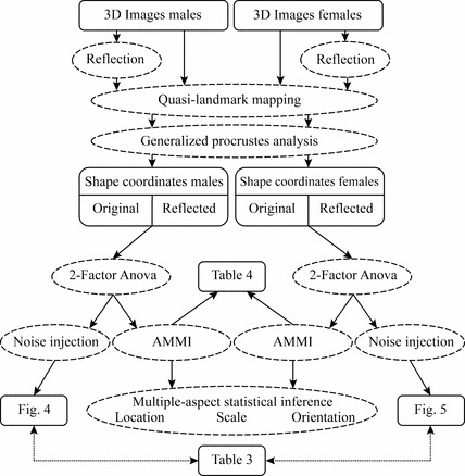
Method work-flow (AMMI, additive main model and multiplicative interaction).

Sampling, facial mapping and Procrustes superimposition

We selected one sample of 98 males and one of 98 females, all with self-reported European ancestry and aged between 18 and 25 years, with an average of 20 years, living in Perth, Western Australia, from the dataset of 3D facial images previously used in Claes et al. (2011). With pooled samples, the following mapping and alignment was performed. First, an anthropometric mask was non-rigidly mapped onto the original 3D images and their reflections (Claes, 2007; Claes et al. 2011, 2012a), which were constructed simply by changing the sign of the x-coordinate (Klingenberg & McIntyre, 1998; Mardia et al. 2000). This established homologous spatially dense quasi-landmark configurations for all original and reflected 3D images (Claes et al. 2011). Note that, by homologous, we mean that each quasi-landmark occupies the same position on the face relative to all other quasi-landmarks. Subsequently, following Mardia et al. (2000), a generalized Procrustes superimposition (Rohlf & Slice, 1990), eliminating differences in position, orientation and scale of both original and reflected configurations combined, was performed. This constructed a tangent space of the Kendall shape space centred on the overall consensus configuration (Dryden & Mardia, 1998). Procrustes shape coordinates, representing the shape of an object (Mitteroecker & Gunz, 2009), were obtained for all 3D faces and their reflections. In the tangent space, the Euclidean distance between two configurations of Procrustes coordinates is known as the Procrustes distance and serves as a measure of shape difference or dissimilarity (Mitteroecker & Gunz, 2009).

After Procrustes superimposition, the overall consensus configuration is perfectly symmetrical and a single shape can be decomposed into its asymmetric and its bilaterally symmetric part (Mardia et al. 2000). Indeed, the average of an original and its reflected configuration constitutes the symmetric component, while the difference between both configurations constitutes the asymmetric component (Klingenberg et al. 2002; Kimmerle & Jantz, 2005). From here on, the male and female cohorts were treated separately as samples from different populations.

Partitioning of facial shape variation

A partitioning of variation in these male and female population samples performed with the commonly used two-factor anova design with individuals (rows) and reflections (columns) as main effects (Klingenberg et al. 2002). The original decomposition of shape variation into components of symmetry and of asymmetry with an associated formal test for directional asymmetry by Mardia et al. (2000) was extended by Klingenberg et al. (2002) to encompass the full two-factor anova design including fluctuating asymmetry and measurement error (Palmer & Strobeck, 1986). This two-factor anova design partitions the variation in shape centred on the overall consensus configuration into components due to individuals, reflections, individual × reflection interactions, and measurement error. Variation among symmetry components, corrected for the effects of asymmetry, is obtained by the main effect of individuals. Directional asymmetry (DA) corresponds to the main effect of reflections and fluctuating asymmetry (FA) is ascertained by the interaction term (individual × reflection). Finally, measurement error is typically computed from the variation among replicate measurements (multiple quasi-landmark configurations of the same individual, which are grouped in a single cell). However, replicate measurements were missing, as only a single facial mapping was performed. This was dealt with in two different ways: Noise Injection (or simulating technical replication error) and Additive Main & Multiplicative Interaction (AMMI) modelling. Note that biological replication error (imaging the same person multiple times) was not considered here but would presumably be greater than the measurement error, as individuals may show variable effects dependent on their facial tone or expression. Also note that antisymmetry was not measured using this framework and was not addressed in this study.

Noise injection

Inspired by the study of Kimmerle & Jantz (2005), in which repeated measures were only available for a subset of the entire sample, we assumed that the deviations between two repeated measures were consistent for the entire sample. In a separate study (data not shown), a so-called repeatability error of the mapping process was estimated from 10 faces mapped each with 10 different initializations. A single initialization started from five manually indicated landmarks (the centres of right and left eye, nose tip, and right and left mouth corner) (Claes et al. 2011). A quasi-landmark repeatability error with 0.2 mm standard deviation [0.002 (dimension less) after size normalization] was measured from a landmark indication error of 1 mm standard deviation. Further testing indicated that the 0.2 mm repeatability error was actually independent of the landmark indication error. This does not come as a surprise as the mapping process was designed to be as invariant as possible to the initial landmark indication error. Instead, the repeatability error was attributed to an algorithmic parameter (set equal to 0.1 mm) which reflects evaluation accuracy of implicit functions needed in the mapping (chapter 3: Claes, 2007). From this result, random normal distributed noise with zero mean and 0.002 standard deviation was injected into the aligned and scaled original and reflected configurations, generating three randomly perturbed replicate measurements of each, needed for the traditional two-factor anova partitioning.

The first partitioning, with injected replicate measurements, was performed under an isotropic model assumption providing a useful measure of the magnitude (but not the direction) of the effects (Klingenberg & McIntyre, 1998). This model presumed independently (uncorrelated), identically (equal amount) and isotropic (same for each direction) distributed variation around each landmark. Therefore it was possible to simply add up the sums of squares (SS) for the different effects across the coordinates of all landmarks and to divide by the appropriate degrees of freedom to obtain an overall analysis (Klingenberg & McIntyre, 1998). The effects can also be analysed on the level of landmarks by adding the SS over the coordinates per landmark only and adjusting the degrees of freedom accordingly. Computationally, this partitioning requires a separate two-way anova on each coordinate following a simple univariate setting, which is time-consuming but nevertheless feasible when working with spatially dense configurations. Statistical significance was assessed using permutation tests with 1000 randomly permuted observations (Klingenberg & McIntyre, 1998; Anderson, 2001a).

The second partitioning, with injected replicate measurements, was performed following a multivariate setting. However, the known multivariate extension using manova (Klingenberg et al. 2002) was computationally impracticable owing to the explicit construction and inversion of variance-covariance matrices. With the quasi-landmarks used in this study these matrices would be large (∼ 30 000 × 30 000) and of low (incomplete) rank (98-1) because the number of variables is high and exceeds the number of observations, implying over-dimensioned spaces and loss of power (Brombin & Salmaso, 2009). Therefore, a distance-based non-parametric multivariate analysis of variance (NPMANOVA) was employed (Anderson, 2001b), which does not suffer from the same drawbacks nor does it assume multivariate normality. The dissimilarity measure used was the Procrustes distance. Statistical significance was assessed using the same permutation strategies as before with 1000 runs (Anderson, 2001a).

Additive main and multiplicative interaction

AMMI models are an alternative way to deal with only a single observation per cell (Dias & Krzanowski, 2006; Corsten & Van Eijnsbergen, 1972). The underlying idea is to model both the main effects of individuals and reflections as additive (as in the classical anova model) and the residual term by a set of multiplicative components plus some residual error. To estimate the unknown parameters in the AMMI model, one uses the row/column means for the main effects and then performs a singular value decomposition of the residual for the multiplicative interaction parameters (Dias & Krzanowski, 2006). Because the residual matrix is a mixture of interactions and measurement error, only a reduced set of the higher (according to the accompanying singular value) components explains true patterns of interaction. The other, lower components mainly model measurement error and are therefore dropped. The key objective is to find a good number of components to retain.

The AMMI framework was a practical foundation when dealing with spatially dense data and was capable of partitioning and visualizing multivariate patterns of both symmetry and asymmetry as follows. (i) The row means were the same as the symmetry components of the individuals and coded for patterns of facial symmetry that were then extracted and visualized using principal component (PC) analysis (PCA). Note that this is similar to the use of PCA to display patterns of (symmetrical) individual variation, corrected for asymmetry, in the work of Klingenberg et al. (2002). In Appendix 1 a simple strategy for PCA on a rank deficient variance-covariance matrix is detailed, which was used extensively in the methods. The number of significant PCs was determined using parallel analysis (PA) (Kranklin et al. 1995), which statistically defined spurious PCs against PCs of equally dimensioned but random and uncorrelated data. (ii) The difference in column means coded for directional asymmetry. This was the same as a difference in sample mean of the original and reflected configurations treated as different populations. Significance assessment of DA was therefore done following the population location test described in the next section. Note that this is identical to the permutational version of the formal test for bilateral symmetry given by Mardia et al. (2000). (iii) Pairwise differences taken between columns were the same as the asymmetry components of the individuals and coded for patterns of facial asymmetry. These were again extracted with PCA that first included a centring (on the average) of the differences, which was essentially equal to subtracting the DA from each of the individual asymmetry components. In other words, by taking the difference of the columns and centring the data subsequently, the main row and column effects were removed and residuals contain interactions and measurement errors only. For visualization purposes the overall consensus configuration, which was symmetric (Mardia et al. 2000), was added back to the residuals. Finally, PA was used as well to extract the number of significant PCs, truly reflecting patterns of interaction or fluctuating asymmetry in this study. Note that, this is similar to the use of PCA to display patterns of fluctuating asymmetry in the work of Mardia et al. (2000) and Klingenberg et al. (2002), with the difference in mean-centring the data and the way FA is separated from measurement noise, respectively.

Statistical inferences on population location, variance-covariance scale and orientation

Sexual dimorphism in patterns of facial symmetry and asymmetry separately (for which suitable quasi-landmark configurations were obtained from the AMMI partitioning of variance) was assessed on multiple aspects, as illustrated schematically in Fig. 2: population location (central tendency), variance-covariance scale (dispersion) and orientation (structure). Traditional statistics to test each of these aspects among different groups were not applicable. Even ordination techniques such as linear discriminant analysis could not be applied because they also require full rank variance-covariance matrices (Mitteroecker & Bookstein, 2011). Therefore, alternative distance-based permutational approaches were employed.

Fig. 2.

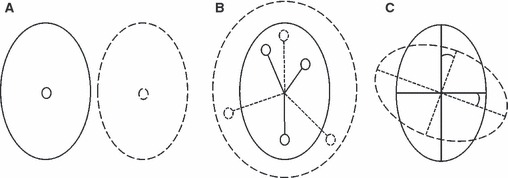
Multiple aspect analysis. (A) Two populations differing in location only. Feature to focus on is the sample mean or centroid. (B) Two populations differing in variance-covariance scale only. The feature to focus on is the sample dispersion based on distances from the centroid. (C) Two populations differing in variance-covariance orientation only. The feature to focus on is the sample subspace, represented using eigenvectors and the principal angles between them.

The key to the problem was simply to establish an appropriate measure of dissimilarity or distance between observations for each of the three aspects to be tested. Then a single but non-pivotal D(istance)-statistic between different groups could be defined as illustrated schematically in Fig. 3A. Employing the work on NPMANOVA of Anderson (Anderson, 2001b; McArdle & Anderson, 2001), allowing for direct additive partitioning of variation for complex models, a related but pivotal F-statistic could also be defined by measuring and partitioning dissimilarity between all pairs of individual observations as depicted in Fig. 3B. Significance was assessed under permutation where the original male and female cohorts generated the observed D- and F-statistics. Subsequently, male and female faces were permuted across groups and both the D- and F-statistics under permutation were tested against the observed values. This was repeated 1000 times and the number of times the permutated values were bigger or equal to the observed values divided by the total number of permutations, generated a P-value.

Fig. 3.

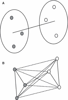
(A) A non-pivotal D-statistic is computed as a single distance between both groups of observations. (B) A pivotal F-statistic is computed by comparing the within pair-wise distances (solid lines), against the between pair-wise distances (dotted lines) of observations.

Location

The first test assessed the difference in central tendency, which generally measures population divergence and in this case more specifically the degree of sexual dimorphism (Fig. 2A). An observation for this test was defined as a single configuration of Procrustes coordinates (either the symmetry or asymmetry component as explained previously). The D-statistic was simply the Euclidean distance between the sample means of each group. The F-statistic was an exact application of Anderson (2001b) using the Euclidean distance between all pairs of configurations. Note that this is also equivalent to the permutational version of the two independent-sample Goodall’s F-test, which is well known in shape analysis (Goodall, 1991; Bookstein, 1997b). Also note that the test for DA under the AMMI model followed an analogous difference in location test between original and reflected configurations as separate populations, which was then identical to the permutational version of the formal test for bilateral symmetry given by Mardia et al. (2000).

Variance-covariance scale

The second test assessed the difference in overall dispersion, which measures differences in the magnitude of variance or the stability of a population around its consensus configuration (Fig. 2b). Following Anderson (2006), we measured the Euclidean distance between each configuration of Procrustes coordinates and its group consensus as a residual, which was seen as a single (univariate) observation. The D-statistic was the absolute difference in average residual of both groups. The F-statistic was an exact application of Anderson (2006).

Variance-covariance orientation

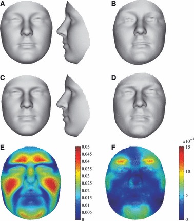
The third and last test assessed the difference in covariance structure, which measures differences in patterns or directions of variance (Fig. 2C). A single observation for this test was the subspace spanned by a sample of quasi-landmark configurations (not just a single but a group of configurations). Given a sample of configurations, a proper representation of the subspace was the unit eigenvectors or PCs of the sample covariance matrix (Appendix 1). Subsequently, a set of distances between two subspaces was defined using the projection metric (Hamm & Lee, 2008):

Here, θ_i for are the critical angles (Krzanowski, 1979) also known as principal angles (Knyazev & Argentati, 2002). These angles combine PCs in a pairwise fashion from both subspaces in decreasing similarity or increasing angle value. In other words, θ₁ is the smallest angle between all pairs of PCs in the first and second subspace. θ₂ is the second smallest angle between all pairs of PCs except the ones already combined by θ₁ and so on. Note that the cosine of these angles is also known as the canonical correlations (Hamm & Lee, 2008).

Based on the work of Krzanowski (1993), a D-statistic-based test was then obtained as follows: (i) Appropriate symmetry and asymmetry subspaces for both male and female cohorts treated separately were derived from the previously AMMI partitioning of variance. (ii) Only a limited number of K PCs were retained based on the outcome of the Parallel Analysis. This was to ensure that enough relevant variation was captured in the subspace representation without incorporating too much irrelevant variation. (iii) A set of K distances was computed by incrementally augmenting the number of principal angles used in the projection metric from 1 to K. (iv) Permutation was performed on centered data to avoid the contamination of between variance-covariance (difference in sample location) (Shipley, 2000) and steps (i)–(iii) were repeated with the same number of K PCs.

As in the previous two tests, a straightforward extension to an F-statistic would be possible but requires a multiple, non-overlapping sampling of male and female cohorts, which is quite data hungry and often not practicable. Instead, an intermediate but computationally more demanding solution was presented: 50 bootstrapped samples with replacement were generated for both the male and female cohort separately. Hence, 50 observations per group were given and distances between all pairs of observations generated the observed F-statistic (Anderson, 2001b). Permutation was performed across the original male and female cohorts on centered data as for the D-statistic and the bootstrapping of 50 observations per group was repeated. Note that, the effect of using bootstrapping is an underestimation of the actual within-group variance because of overlap between different bootstrapped samples. However, some effect of sampling differences is still taken into account compared with the D-statistic, making this F-statistic a sort of ‘semi-pivotal’ statistic.

All statistical routines were implemented in matlab™ 2011a and are available on request by email to the corresponding author.

Results

Partitioning of facial shape variation

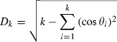
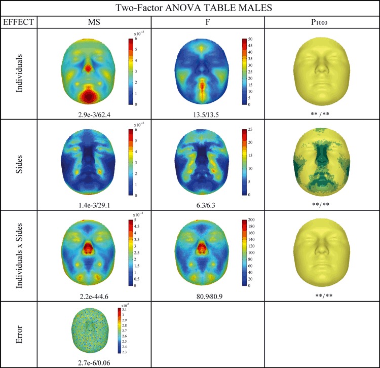
The two-factor anova partitioning of male and female facial shape based on injected noise is given in Figs 4 and 5, respectively. The decomposition of shape into symmetry, DA and FA was reported according to Klingenberg & McIntyre (1998). The figures read like two-factor anova tables, with the sums of squares and degrees of freedom omitted for purposes of clarity and owing to the redundancy in information. The mean squares (MS) reflect absolute effect magnitude, whereas the F-ratios reflect relative magnitude or effect strength. In other words, an effect can be large in absolute magnitude (MS), but can be unimportant (F-ratio) in relative terms. Overall, the main effects of individuals and reflections and the interaction term, in both males and females separately, were highly significant (P < 0.001) according to both the isotropic and the NPMANOVA. Numerically, all the male variations (symmetric, asymmetric, and interactions) were larger than the female variations. The variation in individuals, consisting of symmetric variation, was mainly located in the chin, mouth, nose, cheek and forehead, with some visual differences between males and females, especially on the forehead and mouth. This indicated that variation amongst individuals was predominantly due to differences in their facial profiles that varied from prognathic (concave profile) through orthognathic (straight profile) to retrognathic (convex profile) (Enlow & Hans, 1996). The significance of this, however, which was tested against the interaction component as the error term, is not really meaningful, as noted by Klingenberg et al. (2002). For both males and females, specific areas in the face displayed significant DA, which was coded in the main effect of reflections. An interesting exclusion from DA was the nose. The pattern of DA between males and females was visually different. FA, which was measured in the interaction term, significantly affected the complete face, but bigger interactions were mainly located in specific facial features, such as the nose, for both males and females. The difference between sexes observed was mostly a difference in magnitude only. In other words, although males showed more FA throughout the regions affected, females also showed FA in these same parts of the face. Finally, as expected, the error term visually reflected the pattern of the noise injected.

Fig. 4.

Two-factor anova partitioning of male facial shape variation following an isotropic model (IM) and a distance-based NPMANOVA (D). Throughout the table values are coded as IM/D. P1000 Column: P values using 1000 permutations with * and light green P < 0.05; ** and yellow P < 0.001; dark green not significant (P ≥ 0.05). MS (mean square) is the sum of squares divided by the appropriate degrees of freedom, reflecting the magnitude of the effect. F (F-ratio) is the MS divided by an appropriate error MS, reflecting the relative magnitude or strength of the effect. The interaction term is used as error term for the main effects of individuals and sides and the actual error term is used for the interaction term.

Fig. 5.

Two-factor anova partitioning of female facial shape variation following an isotropic model (IM) and a distance-based NPMANOVA. Throughout the table, values are coded as IM/D. P1000 Column: P values using 1000 permutations with * and light green P < 0.05; ** and yellow P < 0.001; dark green not significant (P ≥ 0.05). MS (mean square) is the sum of squares divided by the appropriate degrees of freedom, reflecting the magnitude of the effect. F (F-ratio) is the MS divided by an appropriate error MS, reflecting the relative magnitude or strength of the effect. The interaction term is used as error term for the main effects of individuals and sides and the actual error term is used for the interaction term.

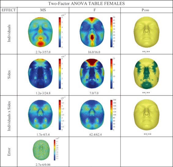
Following the AMMI framework, for females and males separately, the consensus for original and reflected configurations combined, which is the (symmetric) group average, is depicted in Fig. 6A and C, respectively. DA, which was coded as the difference in column means, was found to be highly significant (Table 1, top lines) and the pattern of DA was similar to the one obtained in Figs 4 and 5. DA was amplified five times for better visibility and is shown in Fig. 6B and E for females and males, respectively. The PA results for the PCA modelling of patterns of symmetry and FA are given in Table 2 and the first two PCs for males and females are depicted separately in Fig. 7. The AMMI results are essentially an alternative way of reporting on the decomposition of shape into symmetry, DA and FA. In other words, although constructed and perhaps shown differently, the results should be consistent with the results given in Figs 4 and 5. For example, the AMMI results indeed confirm that differences in facial profile from prognathic (concave profile) to retrognathic (convex profile) play an important role in the patterns of symmetric shape variation. Additionally, for the patterns of FA, as before, facial features played an important role. More importantly, however, an interesting interplay of different facial parts was observed. For example, for both males and females the first PC of FA displayed an asymmetry in the chin with an opposite, perhaps compensating, asymmetry in the upper part of the face. For both patterns of symmetry and FA in both males and females the number of significant PCs was relatively small (between 11 and 13 significant PCs), but they explained at least 85% of the total variance.

Fig. 6.

Sexual dimorphism on the aspect of sample location for the component of symmetry (E) and asymmetry (F). (A) Female symmetric group average. (B) Female directional asymmetry, differences between mean original and reflected configurations amplified five times and visualized onto (A). (A) Male symmetric group average. (B) Male directional asymmetry, differences between mean original and reflected configurations amplified five times and visualized onto (A).

Table 1.

Significance results on D- and F-statistics of sexual dimorphism in sample location, scale and orientation for components of symmetry and asymmetry separately

		D-statistic	P1000	F-statistic	P1000
DA	Males	0.44	0.000	0.87	0.000
	Females	0.41	0.000	0.82	0.000
Sexual dimorphism in patterns of facial symmetry	Location	1.90	0.000	17.90	0.000
	Scale	0.11	0.401	0.73	0.387
	Orientation 1 : 1 : 15 principal angles	0.06	0.163	169.76	0.059
		0.12	0.253	162.80	0.106
		0.17	0.250	159.66	0.035
		0.24	0.043	149.71	0.028
		0.31	0.034	140.53	0.029
		0.37	0.046	130.21	0.036
		0.45	0.024	120.13	0.043
		0.54	0.020	111.57	0.034
		0.63	0.030	103.42	0.027
		0.76	0.010	96.83	0.017
		0.87	0.019	90.03	0.013
		1.00	0.097	82.62	0.004
		1.25	0.006	74.04	0.001
		1.52	0.002	61.08	0.000
		1.81	0.002	41.75	0.000
Sexual dimorphism in patterns of facial asymmetry	Location	0.37	0.007	2.55	0.013
	Scale	0.18	0.005	7.99	0.006
	Orientation 1 : 1 : 15 principal angles	0.09	0.960	182.60	0.744
		0.15	0.799	184.17	0.358
		0.22	0.397	172.33	0.180
		0.28	0.443	159.90	0.098
		0.37	0.419	155.10	0.113
		0.45	0.586	145.42	0.161
		0.55	0.584	135.33	0.149
		0.64	0.818	124.17	0.148
		0.76	0.663	113.97	0.130
		0.90	0.607	103.74	0.127
		1.06	0.517	91.04	0.192
		1.26	0.464	76.32	0.342
		1.48	0.525	60.09	0.518
		1.76	0.447	44.63	0.587
		2.02	0.423	32.51	0.571

DA, directional asymmetry.

Table 2.

Parallel analysis (PA) results for symmetry and asymmetry subspaces with percentage explained by the number of significant (PA columns) or chosen (#PC columns) principal components for the variance-covariance orientation test-setup

	PA	% Expl	#PC	% Expl
Symmetry
Males	12	89	15	92
Females	13	92	15	93
Asymmetry
Males	13	85	15	87
Females	11	85	15	89

Fig. 7.

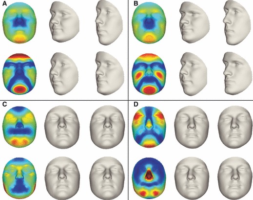
The effects, a positive morph and a negative morph along the first two principal components in patterns of symmetry [(A) females, (B) males], and asymmetry [(C) females, (D) males].

Sexual dimorphism in patterns of facial symmetry and asymmetry

The main purpose of the subsequent results is to report on gender differences, significant or otherwise. The statistical testing for sexual dimorphism in patterns of facial symmetry and asymmetry treated separately is given in Table 1. Overall, the findings from the D- and F-statistics were not different. On the aspect of sample location, sexual dimorphism was found to be strongly significant for the average component of symmetry (P < 0.001) and significant for the average component of asymmetry (DA) (P < 0.05). Mean male and female differences are illustrated in Fig. 6E and F, and were mainly located on the chin, brow ridge and sub-orbital-zygomatic-maxillary (upper cheek) region. The differences measured are consistent with the previously observed differences in main effects across Figs 4 and 5. On the aspect of sample variance-covariance scale, the magnitude of variation in facial symmetry of males (Dispersion = 3.06) was not significantly different from that of females (Dispersion = 2.95). In contrast, the magnitude of variation in facial asymmetry was significantly (P < 0.05) larger in males (Dispersion = 1.66) than in females (Dispersion = 1.47). This confirmed the observed difference in FA magnitude from Figs 4 and 5. The actual distributions of the dispersions (as distances to sample means) for both males/females and symmetry/asymmetry are shown in Fig. 8. Similarity and dissimilarity in distribution are observed for the components of symmetry and asymmetry, respectively.

Fig. 8.

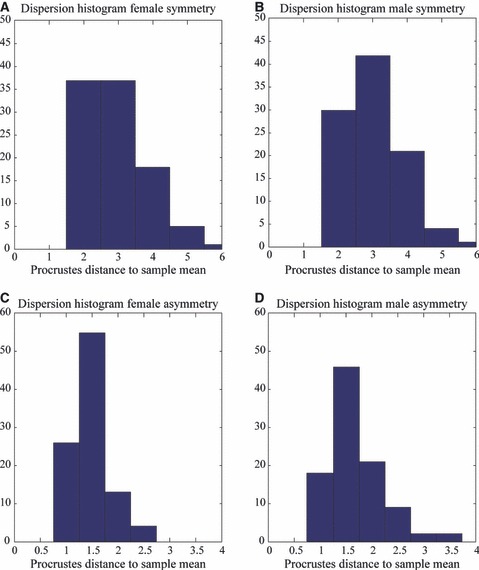
Sexual dimorphism for the aspect of sample scale. Distribution of dispersions for the components of symmetry [(A) females, (B) males] and asymmetry [(C) females, (D) males].

Finally, on the level of sample variance-covariance orientation, the structure of facial symmetry variation was significantly different between males and females and showed only a few overlapping directions (results for smallest number of principal angles). By contrast, no significant difference was observed in the patterns of FA. Fifteen PCs were used, which equalled the maximum number of significant PCs from the PA, given in Table 2, plus two to ensure that all the important but not too many PCs were used to compute the principal angles. A visual and more complete summary of the findings on the level of sample variance-covariance orientation is given in Fig. 9. In these displays it is obvious that the observed D- and F-statistic were at the top end (significant) of the generated null distributions (by permutation) for the patterns of symmetry, whereas they were obscured (non-significant) in the null distributions for the patterns of asymmetry.

Fig. 9.

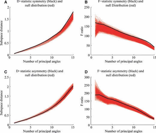
Sexual dimorphism for the aspect of sample orientation for the component of symmetry [(A) D-statistic; (B) F-statistic] and asymmetry [(C) D-statistic; (D) F-statistic].

Discussion

The face is the most identity-coding part of the human body (Smeets et al. 2010) and clearly displays bilateral symmetry. When symmetry is taken into account, improvements of state-of-the-art face recognition techniques are possible (Smeets et al. 2011b). Facial asymmetries are also a feature of normal (and abnormal) growth and development (Ferrario et al. 1995; Ercan et al. 2008; Claes et al. 2011) and are an important factor in mate selection (Baudouin & Tiberghien, 2004), with some asymmetry features accepted as a trait of beauty (Zaidel & Cohen, 2005). Therefore, a study on facial shape variation and anatomy needs to focus on patterns of both symmetry and asymmetry for a full understanding of structural variation.

Three-dimensional scanning and geometric morphometrics are providing the means to establish phenotypic investigations (Baynam et al. 2011, 2012) and are used in this work to analyse sexual dimorphism in 3D facial shape. We start from previous and related work (Claes et al. 2011) using spatially dense quasi-landmark configurations. However, the challenge is to deal with a large number of variables that typically exceeds the number of observations, which is not uncommon in modern morphometrics (Mitteroecker & Gunz, 2009). This generates rank-deficient variance-covariance matrices, excluding the use of statistical techniques relying on the explicit construction and the full rank thereof. Furthermore, traditional multivariate analogues to powerful univariate techniques are often too stringent in their assumptions (Anderson, 2001b, 2006). Therefore, statistical inference techniques making use of measures of dissimilarity or distances and permutation are employed. Both a simple D-statistic and a slightly more complicated F-statistic are given to test multiple aspects between population samples. The advantage of the F-statistic compared with the D-statistic is the ability to separate different sources of variation and to work with multiple groups simultaneously, as in the classical anova design (Anderson, 2001b; Anderson & Millar, 2004), which is typically employed in geometric morphometric-based studies (Viscosi & Cardini, 2011). In other words, with the NPMANOVA framework of Anderson (2001b) it was possible to make inferences about all three population aspects through the appropriate definition of a distance. Furthermore, in the case of testing population location differences, the results are identical to both Goodall’s F-test under permutation (Goodall, 1991; Bookstein, 1997b) and the permutational version of the formal test for Directional asymmetry of Mardia et al. (2000). A more technically oriented discussion on the assumptions made and techniques used is given in Appendix 2. Here, we focus the discussion on the results and their biological meaning only.

The results illustrate interplay with some long-standing hypotheses in developmental and evolutionary biology. From the investigation on facial symmetry, and more particularly the differences in sample location, a substantial degree of sexual dimorphism is detected and measured. This suggests the influence of sexual selection on human faces (Badyaev et al. 2000; Puts, 2010). Importantly, from the analysis of the variance-covariance orientation differences, which were significant, sexual dimorphism in facial appearance is tracked back to selective forces (Herler et al. 2010), which cause a change in phenotypic variance-covariance direction in contrast to pure genetic drift (Badyaev & Hill, 2000). In other words, our results are consistent with the assumption that sexual dimorphism is a result of a selective force, for which sexual selection is the most obvious candidate. The lack of variance-covariance scale difference might be surprising because of a hypothesis stating that male faces have an extended period of growth, therefore forming more prominent facial features, whereas females have an attenuated growth, retaining more juvenile characteristics. Women’s faces are on average more neotenous relative to men’s faces (Montagu, 1989), and more neotenized female faces are found to be more attractive to men (Jones, 1995). In other words, owing to the more prominent growth of male faces, a higher overall dispersion in men might be expected. However, considering the relatively young adult age range of our participants, no particular strong growth magnitude differences may have manifested yet, which would be consistent with the absence of a statistically significant difference in variance-covariance scale. The young age of the participants can be perceptually noticed in the symmetric group averages depicted in Fig. 6A and C. It would be interesting to test changes and differences in dispersion as a function of age through the incorporation of older and younger subjects. Alternatively, the measurement of variance-covariance scale could also be an indication that persistent stabilizing selection has resulted in a degree of canalization of facial morphology, with the result that no difference is observed between sexes.

The asymmetry outcomes are intriguingly different and, again, interplay with long-standing hypotheses is observed. For example, a stronger effect of DA is measured in the males, and this difference could be considered significant [although it should be interpreted with caution due to the significant difference in variance-covariance scale (Appendix 2)]. DA is typically argued to be genetically based (Kimmerle & Jantz, 2005). An increase in DA has also been associated with various disorders that impact on craniofacial development, such as in utero alcohol exposure (Klingenberg et al. 2010) and autism spectrum disorder (Hammond et al. 2008). Additionally, a significantly higher level of FA (variance-covariance scale) is observed in the male sample and FA is considered a measure of developmental instability (Schaefer et al. 2006b; Graham et al. 2010). Our investigation of sexual dimorphism in facial asymmetry thus supports the hypothesis that men experience greater developmental instability and this observation may be consistent with the longer life span in women (Kirkwood, 2010) and higher prevalence of neurodevelopmental and craniofacial disorders in males. One cause of this apparent greater level of craniofacial developmental instability in males is the fact that males are haploid for the X chromosome whereas females are diploid. In other words, males are genetically homozygous for the ∼ 1500 X-linked genes and so will express X-linked recessive diseases as if they were dominant. Thus, men experience an increased prevalence of overt or Mendelian genetic disease relative to women. That the effect is ultimately the result of hemizygosity and not sex per se is made clear by studies of interspecific crosses where the weaker sex is generally the hemizygous sex, a phenomenon called Haldane’s rule (Laurie, 1997). Genetic disease can also result from interactions between separate loci, a fact that might also lead to an increase in the rate of genetic disease in males. Also interesting is that the directions of FA are not different between sexes (they share the same variance-covariance orientation). This observation across distinct populations was also noted in Deleon (2007). The fact that all participants in this study were sampled from the same environmental location and socioeconomic background implies that patterns of FA are indeed genetically independent and therefore can truly represent developmental noise.

The patterns of FA, where interesting interactions of different facial parts are seen in the AMMI partitioning of variance, are noteworthy. The skull is the underlying foundation of the soft-tissue envelope, which is the basis assumption for craniofacial reconstruction (Claes et al. 2006, 2010a,b; Wilkinson, 2010). Therefore, insights into growth patterns of both the face and the underlying skull structure can be obtained from patterns of FA. For example, the greatest degree of FA (PC1) was of corresponding but opposite asymmetry in the upper mid face with a strongly asymmetric chin point. This is suggestive of a lateral displacement of the mandible followed by corresponding contralateral asymmetry of the mid-face. This supports part-counterpart adaptive response in the craniofacial skeleton (Enlow, 1968). Noteworthy is that this pattern of asymmetry is also seen in hemimandibular elongation anomalies, where a condylar hyperplasia results in mandibular displacement and severe facial asymmetry (Obwegeser & Makek, 1986; Walters et al., in press). A similar pattern was revealed in a non-clinical population, which is suggestive of the impact on asymmetry associated with minor growth discordance in the mandibular condyles. However, not all conditions that exhibit a condylar hyperplasia present with the same pattern of asymmetry. For example, hemimandibular hyperplasia (Obwegeser & Makek, 1986; Walters et al., in press) is a condition that also includes condylar hyperplasia where there is a contrasting pattern of mandibular displacement in a more inferior and rotational vector about a midline axis. This pattern of asymmetry is either less common in subclinical cases or has less profound impact on facial symmetry variances. However, more data and analysis are needed to investigate this phenomenon.

The analysis of sexual dimorphism presented, was achieved by modelling patterns of symmetry and asymmetry of facial shape separately on healthy subjects and in a 3D spatially dense manner that provides a complete representation of the facial manifestations of this phenomena. A comparison of our findings with related work is mainly limited to the results on the level of sample mean (location) only (Fig. 6). In our study, the difference in symmetry component of females (Fig. 6A) and males (Fig. 6C) displayed in Fig. 6E, has an emphasis on the brow ridges, nose ridge, eye sockets and orbits, chin and elevated cheekbones in males compared with an emphasis of rounder cheek in females. One of the first investigations on sexual dimorphism in human facial shape was performed using Euclidean distance matrix analysis (EDMA) on 22 landmarks in 2D images by Ferrario et al. (1993). They concluded that male faces on average were wider, longer and more rectangular in shape, which conforms to the results presented. Interestingly, Ferrario et al. (1993) also noted that their sex differences were not equally distributed in the two antimeres. They measured differences in both symmetry and asymmetry of facial shape simultaneously and therefore one component can confound the analysis of the other. More recently, Samal et al. (2007) performed a similar study using 29 landmarks and provided a list of features, significantly discriminating between sexes, without further anatomical feedback. Hennessy et al. (2002) achieved the most similar study to the investigation presented here. They performed a geometric morphometric analysis on 3D faces from a similar population in background (Irish, Scottish, Welsh or English compared with Australian of self-reported European descent), with the differences in using only a sparse set of 24 landmarks, without the decomposition of shape into components of symmetry and asymmetry, and looking at the sample mean only. On visualization, to be compared with Fig. 6A and C, Hennessy et al. (2002) described female faces as wider and flatter with eyes more lateral, anterior and further apart, nasal bridge more posterior, a smaller nose, fuller lips and the chin more forward. Although most of these differences are subtle, they can be noted in the results depicted in Fig. 6A and C as well. More interestingly, in a later study, Hennessy et al. (2005) expanded their analysis onto pseudo-landmarks. The anatomical knowledge of 26 ‘true’ landmarks was roughly interpolated for points in-between them (Hutton et al. 2003; Hammond et al. 2004), which provide a spatially dense description of facial shape. Hennessy et al. (2005) illustrate that this ‘whole-face’ analysis reveals numerous additional aspects of facial shape that remains undetected when using a (traditional) landmark-based approach, which is greatly supported by the study presented. Their detected differences between sexes are well described, presented like and are equal to the results shown in Fig. 6A and c. However, some asymmetry is noted in their measured pattern of sexual dimorphism, because shape was not decomposed into component of symmetry and asymmetry.

In contrast to sexual dimorphism in facial soft-tissue structures, much more work has been done on facial skeletal structures (Uytterschaut, 1986). One of the four pillars of an anthropological protocol, is the estimation of sex (Pretorius et al. 2006; Kimmerle et al. 2008; Scholtz & Pretorius, 2010). Therefore, regions of the cranium, e.g. where sexual dimorphism is most pronounced, are worth investigation for determining sex from shape (Bigoni et al. 2010). A complete overview would be outside the scope of the manuscript, but a recent study on sexual dimorphism in adult crania of known sex belonging to people who lived during the first half of the 20^th century in Bohemia, was done using 3D geometric morphometrics on 82 ecto-cranial landmarks and 39 semi-landmarks (Bookstein, 1997a; Andresen et al. 2000) by Bigoni et al. (2010). The upper face was described as lower and wider for males than for females. Males exhibited a relatively flatter and more vertical upper face, which is not seen in Fig. 6, and relatively wider and higher zygomatic arches, which is noted in Fig. 6. In contrast, females had a higher forehead and face, which is seen in Fig. 6. Furthermore, females expressed a more rounded orbit, which is seen in Fig. 6 as well. Additional detailed differences in facial skeletal structures between sexes are given but these were harder to relate to the facial soft-tissue structures depicted in Fig. 6 and hence are not listed here. It should be noted that patterns of sexual dimorphism between different populations are not necessarily the same (Kimmerle et al. 2008; Puts, 2010; Bastir et al. 2011) and it would be interesting to expand the current study setup to multiple populations.

Previous work on the measurement of asymmetry in human faces also exists but is often limited to DA only, without an explicit analysis of sexual dimorphism in facial asymmetry. Again, some of the first studies were performed by Ferrario et al. (1994, 1995). Using EDMA on 16 3D landmarks, they found a significant DA for shape (not for size), in both men and women separately, but numerically no apparent sex differences were observed or tested explicitly for significance. In contrast, a more recent study of Ercan et al. (2008), similarly using EDMA but on 42 landmarks in 2D images, observed (but not tested for significance) a higher number of asymmetric distances, suggesting a higher level of DA, in females than in males. They also give a discussion regarding the dominant part of the face (difference in size only, which is not addressed in our study), with no real consensus emerging. In our study, significant DA is also measured in both males and females but, in contrast, a higher (marginally significant) level of DA is observed in males than in females. However, this can be explained by analysing the localized significance of the reflection main effect depicted in Figs 4 and 5 combined with the differences in DA between sexes in Fig. 6F compared with the sampling of sparse landmarks used in previous studies. Focusing on Ercan et al. (2008), the asymmetric distances found in males and females separately based on 42 landmarks can be easily overlaid with the significant findings in Figs 4 and 5. In other words, the DA found in males and females separately is not contradicted. However, some landmarks, such as the trichion, nasion and gonion, are located in regions displaying DA for females only. Furthermore, some regions, such as the upper brow ridges, temporal-frontal region, upper cheek and chin, clearly display more DA for males but are under-sampled or lack any landmark indication in the study of Ercan et al. (2008). This can bias the analyses in the direction of finding more DA in females than in males. (Note that the under-sampled regions also overlap with the regions displaying sexual dimorphism in the symmetry component; Fig. 6E) Therefore, results and contrasting outcomes in these previous studies are influenced by the choice of landmarks and clearly illustrate the benefit of a spatially dense investigation. More than a decade ago, Ferrario et al. (1995) stated that by adding more landmarks, a better understanding of the facial form could be obtained. Further, we argue that the sampling of landmarks should be spatially dense and even in density across the face (Appendix 2).

A great deal of the work on bilateral symmetry is based on the geometric morphometric approach outlined in Mardia et al. (2000). A complete overview would be outside the scope of the manuscript but some recent studies involving faces are worth mentioning. In chronological order, Hennessy et al. (2004) found sex-specific asymmetries in schizophrenia using five landmarks. The male ‘control’ cohort displayed greater DA compared with the female ‘control’ cohort (significance with a Hoteling’s T²-test). Schaefer et al. (2006a), as part of an analysis on female appearance and rated attractiveness, measured DA in 2D images using 64 facial landmarks. DA was visualized using TPS (thin plate spline) deformation grids (Mitteroecker & Gunz, 2009) displaying an elevation of the left eyebrow ridge and a deviation of the chin point to the right, both of which are seen in Fig. 6B as well. Nose and mouth deformation are less comparable. Hammond et al. (2008) analysed face–brain asymmetry in autism spectrum disorders using spatially dense pseudo-landmarks. DA was measured in both a patient and control group of young boys. Klingenberg et al. (2010) analysed the effect of prenatal alcohol exposure on facial asymmetry. A pattern of DA was measured in 17 landmarks and was visualized onto the complete face by morphing (warping) facial scans based on the landmark positions and displacements. Doing so allows for a visual feedback that is of the same spatial density as the ones shown in Fig. 6B and D. Finally, in Bugaighis et al. (2010) a similar study was done on children with cleft lip and/or palate. The patterns of DA seem to differ between the last three studies mentioned and the one presented in this work, and comparisons are difficult due to the difference in age of the study cohorts.

A final comparison of the findings on facial asymmetry can be made with previous work from the authors (Claes et al. 2011). There, a spatially dense measure of asymmetry on the level of the individual under both typical and abnormal growth was provided. To deal with abnormalities in facial shape, a dysmorphometric-based superimposition, with an associated extended Procrustes ML-estimator, of reflected images onto their original counterparts was used (Claes et al. 2012b). The score encoded for the combined magnitude of DA and FA in an individual. Typical asymmetry indices were derived and conform to findings of this study that the asymmetry in males was more extensive and of a greater magnitude than in females (though these were not tested for significance). It is interesting to see that the summary statistics of the localized asymmetry (from a mixed population sample, largely East Asian and European) does reflect an arrangement that is roughly similar to the simple addition of the patterns of magnitude in DA and FA from Figs 4 and 5. Finally, Claes et al. (2011), discuss other work and challenges to technically establish asymmetry measurements using spatially dense shape descriptions.

We predict that the results of this and similar studies will be relevant for future association studies. The results are useful in providing the basis for typical facial metrics of interest, including masculinity and asymmetry (Gangestad & Thornhill, 2003). For example, let us focus on the non-perceptual metrics defined in Penton-Voak et al. (2001), which are the most commonly used to measure masculinity and symmetry based on distances and proportions between landmarks in the face (Little et al. 2008; Burris et al. 2011). The landmarks employed to determine facial masculinity are clearly located in areas found to be different between sexes (Fig. 6E). Thanks to the results of the spatially dense investigation, additional areas, differentiating between sexes, can now be included. Furthermore, when working on the symmetry component only, facial masculinity can be measured independently from asymmetry such that possible relationships are not confounded. Additionally, the landmarks used to calculate the lack of symmetry are all located in areas mainly displaying FA instead of DA, except for the landmarks determining distance D3, which are located in an area displaying DA, but no FA. Therefore the traditional measurement of asymmetry will largely measure FA, which is often desired. Future work, based on the results described herein, could define new measures of masculinity and asymmetry and test their discriminatory power. Finally, biological variability within individuals, based on repeated images, is also of interest.

Conclusion

The study of sexual dimorphism, which is one of the important outcomes of sexual selection, in the human face, is interesting for many reasons, including a better understanding of facial anatomy. The importance of bilateral symmetry in the face creates the need to study components of facial shape such as symmetry and asymmetry separately, which is confirmed by the contrasting but complementary findings between them. A spatially dense representation of the complete facial form is clearly beneficial when compared to previous studies and findings. The permutational statistical methods employed allow large numbers of variables to be dealt with, which is a common requirement when working with geometric morphometric data, and the results may be useful for future investigations, including association studies. The capacity to objectively decompose components of symmetry/asymmetry will facilitate greater understanding on facial anatomy, developmental processes and selection pressures.

Appendices

Appendix 1

Problem statement: PCA on a mean centered matrix X with dimensions V × N, with N the number of observations, V the number of variables and where . Solution: The eigen-decomposition of the variance-covariance matrix XX^t being a V×V matrix implies that: , where e_i and l_i are an eigenvector and an eigenvalue of the covariance matrix, respectively. Now consider the eigen-decomposition of the smaller N × N matrix X^tX: . Multiplying both sides by X and grouping together in brackets: 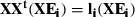one can see that the N vectors are all eigenvectors of the variance-covariance matrix XX^t with corresponding eigenvalues l_i and all remaining eigenvectors XX^t have zero eigenvalues due to the incomplete rank. Hence in the case V is large and N is much smaller, the eigenvectors and eigenvalues are best computed using the smaller X^tX matrix. matlab functions ‘princomp’ and ‘svd’ (singular value decomposition) allow you to flag ‘econ’ in order to perform the more memory-efficient decomposition using X^tX instead of X^tX.

Appendix 2

Although underlying assumptions are avoided as much as possible, we should note the following: (i) for the test of differences in location, observations from both groups are assumed to have a similar distribution, which is also expected for the traditional parametric tests (e.g. Hoteling’s T²-test). The main difference is that ‘similar distributions’ in the non-parametric setting only implies similar multivariate dispersions (same scale) and not similar sample orientation or multivariate normality (Anderson, 2001b). However, it does mean that the significance in sexual dimorphism of DA should be interpreted with caution, given the significant difference in levels of FA (which is essentially a measure of dispersion around DA) between males and females. (ii) The use of multivariate distances, and, in particular, the Euclidean distance, is not completely assumption-free. The Euclidean distance between two landmark configurations is an unweighted distance in the sense that each landmark contributes equally to the overall dissimilarity (Hutteger & Mitteroecker, 2011). In other words, an isotropic model is assumed inherently, which simply explains why the F-ratios obtained from the NPMANOVA given in Figs 4 and 5 are identical to the ones obtained from the two-factor anova decomposition under isotropy. It also explains why the test for population location differences is identical to the permutational version of Goodall’s F-test (Goodall, 1991; Bookstein, 1997b). Furthermore, because of the equal contribution of each landmark to the distances, the sampling of landmarks across the face should be fair. For example, if many more landmarks are placed in particular anatomical regions, those regions will influence the distance much more compared with others and a sort of arbitrary weighting of facial parts is introduced (Hutteger & Mitteroecker, 2011). In the case of the quasi-landmarks, in this study the sampling is done at a constant density as defined in the anthropometric mask. In other words, they are sampled uniformly and equally spaced at ∼ 2 mm from each other. This means that bigger areas have more quasi-landmarks and hence more influence in the multivariate dissimilarity, which is rational. The alternative is to use Mahalanobis distances (Hutteger & Mitteroecker, 2011), as done in Hoteling’s T²-test for tangent space inference (Dryden & Mardia, 1998). However, this requires a pooled variance-covariance matrix (with typical assumptions such as strict similar distributions [see (i)], which are not always appropriate [Parsons et al. 2009)] and is not without problems for permutation testing (Adams, 2011). From the results on variance-covariance scale and orientation we can see that for both the patterns of symmetry and of asymmetry between males and females the assumption of ‘similar distributions’ involving equal scale and orientation does not hold. Furthermore, Hoteling’s T²-test is not powerful unless a large number of observations are available (Brombin & Salmaso, 2009). However, the model of isotropy employed in this work, is considered to be restrictive as well and an interesting alternative approach, which is not explored in this work, is the use of nonparametric combination methodology to shape analysis (Brombin & Salmaso, 2009; Pesarin & Salmaso, 2010).

It is appropriate to pay particular attention to the variance-covariance scale and orientation tests. Traditional and alternative routines have existed for a long time (Box, 1949; Manly & Rayner, 1987) and the most commonly known approach in morphometrics is based on the work of Flury using common principal components (CPC) (Flury, 1988a,b). The elegance of Flury’s work is the existence of a hierarchy (Phillips & Arnold, 1999; Steppan et al. 2002) testing whether variance-covariance matrices are (i) ‘equal’ [which can also be tested by matrix correlations (Ackermann & Cheverud, 2000)], (ii) ‘proportional’ (same orientation, different scale, which is the case for the patterns of facial FA in this work), (iii) ‘have common PCs’ (both overlapping and different directions, which is the case for the patterns of facial symmetry in this work) or (iv) ‘unrelated’ [completely different directions, which would be the case for patterns of symmetry vs. asymmetry, as they belong to complementary orthogonal subspaces of Procrustes tangent space (Mardia et al. 2000)]. The disadvantage is the need to construct the variance-covariance matrices explicitly to compute the CPCs. Flury (1987) generalized the CPC model and provided the link with the common space analysis of Krzanowski (1979), which is used in this work. However, the benefit of working with subspaces directly is the ability to use PCA instead of CPC for which a simple computational strategy exists when working with more variables than observations (see Appendix 1). Note that, in the case of spatially dense quasi-landmarks, strong correlations are expected (Hutteger & Mitteroecker, 2011) and hence a technique such as PCA, is able to eliminate all (or most of) the redundancy in the data. This is seen in the results from the variance explained in the significant PCs after PA. Only a small number (11–13) of PCs already explain 85–92% of the total variance in ∼ 10 000 quasi-landmarks. Also note that the better the consistency of the spatially dense indications, the better the reduction obtained. Finally, note that subspace representations of variance-covariance matrices and distances between them have been used recently to track their developmental trajectories (Mitteroecker & Bookstein, 2009; Gonzalez et al. 2011). The difference lies in the definition of the metric used. Instead of simply summing the squared canonical correlations (cosine of the principal angles), as in the projection metric employed here, the logarithm of the canonical correlations is taken in Mitteroecker & Bookstein (2009). Doing so, changes the relative influence of smaller vs. larger principal angles in the final distance, which might be preferable in some contexts.

Ethics approval

(1) The Characterisation of 3-Dimensional Facial Profile in Young Adult Western Australians was granted from the Princess Margaret Hospital for Children (PMH) ethics committee (PMHEC 1443/EP) in Perth, WA, Australia. (2) Establishment of Identity from Quantitative Analysis of Facial Characteristics (Digital 3D facial modelling) was granted from the University of Melbourne, human research ethics committee (HESC 050550.1) in Melbourne, VIC 3010, Australia. (3) Genetics of Human Pigmentation, Ancestry and Facial Features IRB#32341 was approved by the IRB of Penn State University.

Author contributions

The work is the result of an interdisciplinary and inter-institutional collaboration between science computing (P.C., D.V., P.S.), Biostatistics (P.C., G.V.), anatomy (M.W., J.C), quantitative (G.G.), clinical (G.B.) and human genetics (M.D.S.) and behavior (D.P). M.W is responsible for the data collection. P.C. developed the technical algorithms, implemented the statistical routines, designed, performed the data analysis and wrote the manuscript with appropriate input and revisions from all authors.

References

- Ackermann RR, Cheverud JM. Phenotypic covariance structure in tamarins (Genus Saguinys): a comparison of variation patterns using matrix correlation and common principal component analysis. Am J Phys Anthropol. 2000;111:489–501. doi: 10.1002/(SICI)1096-8644(200004)111:4<489::AID-AJPA5>3.0.CO;2-U. [DOI] [PubMed] [Google Scholar]
- Adams D. Morphmet. 2011. Re: tribulations with permutations. available at http://www.mail-archive.com/morphmet@morphometrics.org/msg02265.html. [Google Scholar]
- Adams DC, Rohlf F, Slice D. Geometric morphometrics: ten years of progress following the revolution. Ital J Zool. 2004;71:5–16. [Google Scholar]
- Aeria G, Claes P, Vandermeulen D, et al. Targeting specific facial variation for different identification tasks. Forensic Sci Int. 2010;201:118–124. doi: 10.1016/j.forsciint.2010.03.005. [DOI] [PubMed] [Google Scholar]
- Anderson JM. Permutation tests for univariate or multivariate analysis of variance and regression. Can J Fish Aquat Sci. 2001a;58:626–639. [Google Scholar]
- Anderson MJ. A new method for non-parametric multivariate analysis of variance. Austral Ecol. 2001b;26:32–46. [Google Scholar]
- Anderson MJ. Distance-based tests for homogeneity of multivariate dispersions. Biometrics. 2006;62:245–253. doi: 10.1111/j.1541-0420.2005.00440.x. [DOI] [PubMed] [Google Scholar]
- Anderson MJ, Millar RB. Spatial variation and effects of habitat on temperate reef fish assemblages in northeastern New Zealand. J Exp Mar Biol Ecol. 2004;305:191–221. [Google Scholar]
- Andresen PR, Bookstein FL, Conradsen K, et al. Surface-bounded growth modeling applied to human mandibles. IEEE Trans Med Imaging. 2000;19:1053–1063. doi: 10.1109/42.896780. [DOI] [PubMed] [Google Scholar]
- Badyaev AV, Hill GE. The evolution of sexual dimorphism in the House Finch. I. Population divergence in morphological covariance structure. Evolution. 2000;54:1784–1794. doi: 10.1111/j.0014-3820.2000.tb00722.x. [DOI] [PubMed] [Google Scholar]
- Badyaev A, Hill GE, Stoehr AM, et al. The evolution of sexual size dimorphism in the House Finch. II. Population divergence in relation to local selection. Evolution. 2000;54:2134–2144. doi: 10.1111/j.0014-3820.2000.tb01255.x. [DOI] [PubMed] [Google Scholar]
- Bastir M, Godoy P, Rosas A. Common features of sexual dimorphism in the cranial airways of different human populations. Am J Phys Anthropol. 2011;146:414–422. doi: 10.1002/ajpa.21596. [DOI] [PubMed] [Google Scholar]
- Baudouin JY, Tiberghien G. Symmetry, averagness, and feature size in the facial attractiveness of women. Acta Psychol (Amst) 2004;117:313–332. doi: 10.1016/j.actpsy.2004.07.002. [DOI] [PubMed] [Google Scholar]
- Baynam G, Claes P, Craig JM, et al. Intersections of epigenetics, twinning and developmental asymmetries: insights into monogenic and complex diseases and role for 3D facial analysis. Twin Res Hum Genet. 2011;14:305–315. doi: 10.1375/twin.14.4.305. [DOI] [PubMed] [Google Scholar]
- Baynam G, Walters M, Claes P, et al. 3D facial analysis can investigate vaccine responses. Med Hypotheses. 2012;78:497–501. doi: 10.1016/j.mehy.2012.01.016. [DOI] [PubMed] [Google Scholar]
- Bigoni L, Velemínska J, Brůžek J. Three-dimensional geometric morphometrics analysis of cranio-facial sexual dimorphism in a Central European sample of known sex. J Comp Hum Biol. 2010;61:16–32. doi: 10.1016/j.jchb.2009.09.004. [DOI] [PubMed] [Google Scholar]
- Bock MT, Bowman AW. On the measurement and analysis of asymmetry with applications to facial modelling. Appl Stat. 2006;55:77–91. [Google Scholar]
- Bookstein FL. Landmark methods for forms without landmarks: morphometrics of group differences in outline shape. Med Image Anal. 1997a;1:225–243. doi: 10.1016/s1361-8415(97)85012-8. [DOI] [PubMed] [Google Scholar]
- Bookstein FL. Shape and the information in medical images: a decade of the morphometric synthesis. Comput Vis Image Underst. 1997b;66:97–118. [Google Scholar]
- Box GEP. A general distribution theory for a class of likelihood criteria. Biometrika. 1949;36:317–346. [PubMed] [Google Scholar]
- Brombin C, Salmaso L. Multi-aspect permutation tests in shape analysis with small sample size. Comput Stat Data Anal. 2009;53:3921–3931. [Google Scholar]
- Bugaighis I, O’Higgens P, Tiddeman B, et al. Three-dimensional geometric morphometrics applied to the study of children with cleft lip and/or palate from the North East of England. Eur J Orthod. 2010;32:514–521. doi: 10.1093/ejo/cjp140. [DOI] [PubMed] [Google Scholar]
- Burris RP, Roberts SC, Welling LLM, et al. Heterosexual romantic couples mate assortatively for facial symmetry, but not masculinity. Pers Soc Psychol Bull. 2011;37:601–613. doi: 10.1177/0146167211399584. [DOI] [PubMed] [Google Scholar]
- Claes P. Faculteit ingenieurswetenschappen, department Elektrotechniek, afdeling PSI, Thesis. Leuven: K.U.Leuven; 2007. A robust statistical surface registration framework using implicit function representations: application in craniofacial reconstruction. Available at http://mic.uzleuven.be/download/public/MIC/publications/2967/PHD_pclaes.pdf. [Google Scholar]
- Claes P, Vandermeulen D, De Greef S, et al. Craniofacial reconstruction using a combined statistical model of face shape and soft tissue depths: methodology and validation. Forensic Sci Int. 2006;159:147–158. doi: 10.1016/j.forsciint.2006.02.035. [DOI] [PubMed] [Google Scholar]
- Claes P, Vandermeulen D, De Greef S, et al. Bayesian estimation of optimal craniofacial reconstructions. Forensic Sci Int. 2010a;201:146–152. doi: 10.1016/j.forsciint.2010.03.009. [DOI] [PubMed] [Google Scholar]
- Claes P, Vandermeulen D, De Greef S, et al. Computerized craniofacial reconstruction: conceptual framework and review. Forensic Sci Int. 2010b;201:138–145. doi: 10.1016/j.forsciint.2010.03.008. [DOI] [PubMed] [Google Scholar]
- Claes P, Walters M, Vandermeulen D, et al. Spatially-dense 3D facial asymmetry assessment in both typical and disordered growth. J Anat. 2011;219:444–455. doi: 10.1111/j.1469-7580.2011.01411.x. [DOI] [PMC free article] [PubMed] [Google Scholar]
- Claes P, Walters M, Clement JG. Improved facial outcome assessment using a 3D anthropometric mask. Int J Oral Maxillofac Surg. 2012a;41:324–330. doi: 10.1016/j.ijom.2011.10.019. [DOI] [PubMed] [Google Scholar]
- Claes P, Daniels K, Walters M, et al. Dysmorphometrics: the modelling of morphological abnormalities. Theor Biol Med Model. 2012b;9:1–39. doi: 10.1186/1742-4682-9-5. [DOI] [PMC free article] [PubMed] [Google Scholar]
- Corsten LCA, Van Eijnsbergen CA. Multiplicative effects in a two-way analysis of variance. Stat Neerl. 1972;26:61–68. [Google Scholar]
- Deleon VB. Fluctuating asymmetry and stress in a medieval nubian population. Am J Phys Anthropol. 2007;132:520–534. doi: 10.1002/ajpa.20549. [DOI] [PubMed] [Google Scholar]
- Dias C, Krzanowski WJ. Choosing components in the additive main effect and multiplicative interaction (AMMI) models. Scientia Agricola. 2006;63:169–175. [Google Scholar]
- Dryden IL, Mardia KV. Statistical Shape Analysis. New York: John Wiley & Sons; 1998. [Google Scholar]
- Enlow DH. The human face: an account of the postnatal growth and development of the craniofacial skeleton. Science. 1968;162:1470. [Google Scholar]
- Enlow DH, Hans MM. Essential of Facial Growth. Philadelphia: Saunders; 1996. [Google Scholar]
- Ercan I, Ozdemir ST, Etoz A, et al. Facial asymmetry in young healty subjects evaluated by statistical shape analysis. J Anat. 2008;213:663–669. doi: 10.1111/j.1469-7580.2008.01002.x. [DOI] [PMC free article] [PubMed] [Google Scholar]
- Ferrario VF, Sforza C, Pizzini G, et al. Sexual dimorphism in the human face assessed by euclidean distance matrix analysis. J Anat. 1993;183:593–600. [PMC free article] [PubMed] [Google Scholar]
- Ferrario VF, Sforza C, Poggio CE, et al. Distance from symmetry: a three-dimensional evaluation of facial asymmetry. J Oral Maxillofac Surg. 1994;52:1126–1132. doi: 10.1016/0278-2391(94)90528-2. [DOI] [PubMed] [Google Scholar]
- Ferrario VF, Sforza C, Miani A, et al. A three-dimensional evaluation of human facial asymmetry. J Anat. 1995;186:103–110. [PMC free article] [PubMed] [Google Scholar]
- Flury B. Two generalizations of the common principal component model. Biometrika. 1987;74:59–69. [Google Scholar]
- Flury B. An application of common principal component analysis to cranial morphometry of Microtus californicus and M. ochrogaster (Mammalia, Rodentia) J Zool. 1988a;216:21–36. [Google Scholar]
- Flury B. Common Principal Components and Related Multivariate Models. New York: Wiley; 1988b. [Google Scholar]
- Gangestad SW, Thornhill R. Facial masculinity and fluctuating asymmetry. Evol Hum Behav. 2003;24:231–241. [Google Scholar]
- Gonzalez PN, Hallgrímsson B, Oyhenart E. Developmental plasticity in covariance structure of the skull: effects of prenatal stress. J Anat. 2011;218:243–257. doi: 10.1111/j.1469-7580.2010.01326.x. [DOI] [PMC free article] [PubMed] [Google Scholar]
- Goodall C. Procrustes methods in the statistical analysis of shape. J R Stat Soc Series B (Methodol) 1991;53:285–339. [Google Scholar]
- Graham JH, Raz S, Hel-Or H, et al. Fluctuating asymmetry: methods, theory and applications. Symmetry. 2010;2:466–540. [Google Scholar]
- Hamada H, Meno C, Watanabe D, et al. Establishment of vertebrate left-right asymmetry. Nat Rev Genet. 2002;3:103–113. doi: 10.1038/nrg732. [DOI] [PubMed] [Google Scholar]
- Hamm J, Lee DD. Proceedings of the 25th International conference on Machine Learning. Helsinki: ACM; 2008. Grassman discriminant analysis: a unifying view on subspace-based learning; pp. 376–383. [Google Scholar]
- Hammer Ø, Harper D. Paleontological Data Analysis. Oxford: Blackwell Science Inc; 2006. [Google Scholar]
- Hammond P, Hutton TJ, Allanson JE, et al. 3D analysis of facial morphology. Am J Hum Genet. 2004;126A:339–348. doi: 10.1002/ajmg.a.20665. [DOI] [PubMed] [Google Scholar]
- Hammond P, Forster-Gibson C, Chudley AE, et al. Face-brain asymmetry in autism spectrum disorders. Mol Psychiatry. 2008;13:614–623. doi: 10.1038/mp.2008.18. [DOI] [PubMed] [Google Scholar]
- Hennessy RJ, Kinsella A, Waddington JL. 3D laser surface scanning and geometric morphometric analysis of craniofacial shape as an index of cerebro-craniofacial morphogenesis: initial application to sexual dimorphism. Biol Psychiatry. 2002;51:507–514. doi: 10.1016/s0006-3223(01)01327-0. [DOI] [PubMed] [Google Scholar]
- Hennessy RJ, Lane A, Kinsella A, et al. 3D morphometrics of craniofacial dysmorphology reveals sex-specific asymmetries in schizophrenia. Schizophr Res. 2004;67:261–268. doi: 10.1016/j.schres.2003.08.003. [DOI] [PubMed] [Google Scholar]
- Hennessy RJ, McLearie S, Kinsella A, et al. Facial surface analysis by 3D laser scanning and geometric morphometrics in relation to sexual dimorphism in cerebral-craniofacial morphogenesis and cognitive function. J Anat. 2005;207:283–295. doi: 10.1111/j.1469-7580.2005.00444.x. [DOI] [PMC free article] [PubMed] [Google Scholar]
- Herler J, Kerschbaumer M, Mitteroecker P, et al. Sexual dimorphism and population divergence in the Lake Tanganyika cichlid fish genus Tropheus. Front Zool. 2010;7:1–10. doi: 10.1186/1742-9994-7-4. [DOI] [PMC free article] [PubMed] [Google Scholar]
- Hill H, Claes P, Crocoran M, et al. How different is different? Criterion and sensitivity in face-space. Front Psychol. 2011;2:1–14. doi: 10.3389/fpsyg.2011.00041. [DOI] [PMC free article] [PubMed] [Google Scholar]
- Hutteger SM, Mitteroecker P. Invariance and meaningfulness in phenotype space. Evol Biol. 2011;38:335–351. [Google Scholar]
- Hutton TJ, Buxton BF, Hammond P, et al. Estimating average growth trajectories in shape-space using kernel smoothing. IEEE Trans Med Imaging. 2003;22:747–753. doi: 10.1109/TMI.2003.814784. [DOI] [PubMed] [Google Scholar]
- Jones D. Sexual selection, physical attractiveness, and facial neoteny. Curr Anthropo. 1995;36:723–748. [Google Scholar]
- Kimmerle EH, Jantz RL. Secular trends in craniofacial asymmetry studied by geometric morphometry and generalized procrustes methods. In: Slice D, editor. Modern Morphometrics in Physical Anthropology. New York: Kluwer Academic/Plenum Publishers; 2005. pp. 247–263. [Google Scholar]
- Kimmerle EH, Ross A, Slice D. Sexual dimorphism in America: geometric morphometric analysis of the craniofacial region. J Forensic Sci. 2008;53:54–57. doi: 10.1111/j.1556-4029.2007.00627.x. [DOI] [PubMed] [Google Scholar]
- Kirkwood T. Why women live longer. Sci Am. 2010;303:34–35. [PubMed] [Google Scholar]
- Klingenberg CP, McIntyre GS. Geometric morphometrics of developmental instability: analyzing patterns of fluctuating asymmetry with procrustes methods. Evolution. 1998;52:1363–1375. doi: 10.1111/j.1558-5646.1998.tb02018.x. [DOI] [PubMed] [Google Scholar]
- Klingenberg CP, Barluenga M, Meyer A. Shape analysis of symmetric structures: quantifying variation among individuals and asymmetry. Evolution. 2002;56:1909–1920. doi: 10.1111/j.0014-3820.2002.tb00117.x. [DOI] [PubMed] [Google Scholar]
- Klingenberg CP, Wetherill L, Rogers J, et al. Prenatal alcohol exposure alters the patterns of facial asymmetry. Alcohol. 2010;44:649–657. doi: 10.1016/j.alcohol.2009.10.016. [DOI] [PMC free article] [PubMed] [Google Scholar]
- Knyazev AV, Argentati ME. Principal angles between subspaces in an A-based scalar product: algorithms and perturbation estimates. SIAM J Sci Comput. 2002;23:2008–2040. [Google Scholar]
- Koehler N, Simmons WL, Rhodes G, et al. The relationship between sexual dimorphism in human faces and fluctuating asymmetry. Proc R Soc Lond B. 2004;271:233–236. doi: 10.1098/rsbl.2003.0146. [DOI] [PMC free article] [PubMed] [Google Scholar]
- Kranklin SB, Gibson DJ, Robertson PA, et al. Parallel analysis: a method for determining significant principal components. J Veg Sci. 1995;6:99–106. [Google Scholar]
- Krzanowski WJ. Between-groups comparison of principal components. J Am Stat Assoc. 1979;74:703–707. [Google Scholar]
- Krzanowski WJ. Permutational tests for correlation matrices. Stat Comput. 1993;3:37–44. [Google Scholar]
- Laurie CC. The weaker sex is heterogametic: 75 years of Haldane’s rule. Genetics. 1997;147:937–951. doi: 10.1093/genetics/147.3.937. [DOI] [PMC free article] [PubMed] [Google Scholar]
- Little AC, Jones BC, Waitt C, et al. Symmetry is related to sexual dimorphism in faces: data across culture and species. PLoS One. 2008;3:e2106. doi: 10.1371/journal.pone.0002106. [DOI] [PMC free article] [PubMed] [Google Scholar]
- Manly BFJ, Rayner JCW. The comparison of sample covariance matrices using likelihood ratio tests. Biometrika. 1987;74:841–847. [Google Scholar]
- Mardia KV, Bookstein FL, Moreton IJ. Statistical assessment of bilateral symmetry of shapes. Biometrika. 2000;87:285–300. [Google Scholar]
- McArdle BH, Anderson MJ. Fitting multivariate models to community data: a comment on distance-based redundancy analysis. Ecology. 2001;82:290–297. [Google Scholar]
- Mitteroecker P, Bookstein FL. The ontogenetic trajectory of the phenotypic covariance matrix, with examples from craniofacial shape in rats and humans. Evolution. 2009;63:727–737. doi: 10.1111/j.1558-5646.2008.00587.x. [DOI] [PubMed] [Google Scholar]
- Mitteroecker P, Bookstein FL. Linear discrimination, ordination, and the visualization of selection gradients in modern morphometrics. Evol Biol. 2011;38:100–114. [Google Scholar]
- Mitteroecker P, Gunz P. Advances in geometric morphometrics. J Evol Biol. 2009;36:235–247. [Google Scholar]
- Montagu A. Growing Young. Westport, CT: Bergin & Garvey; 1989. [Google Scholar]
- Obwegeser HL, Makek MS. Hemimandibular hyperplasia – hemimandibular elongation. J Maxillofac Surg. 1986;14:183–208. doi: 10.1016/s0301-0503(86)80290-9. [DOI] [PubMed] [Google Scholar]
- Palmer AR. Fluctuating asymmetry: a primer. In: Markov T, editor. Developmental Instability: Its Origins and Implications. Dordrecht: Kluwer; 1994. pp. 335–364. [Google Scholar]
- Palmer AR, Strobeck C. Fluctuating asymmetry: measurement, analysis, patterns. Annu Rev Ecol Syst. 1986;17:391–421. [Google Scholar]
- Parsons KJ, Cooper WJ, Albertson RC. Limits of principal component analysis for producing a common trait space: implications for inferring selection, contingency and chance in evolution. PLoS One. 2009;4:e7957. doi: 10.1371/journal.pone.0007957. [DOI] [PMC free article] [PubMed] [Google Scholar]
- Penton-Voak IS, Jones BC, Little AC, et al. Symmetry, sexual dimorphism in facial proportions and male face attractiveness. Proc R Soc Lond B. 2001;268:1617–1623. doi: 10.1098/rspb.2001.1703. [DOI] [PMC free article] [PubMed] [Google Scholar]
- Pesarin F, Salmaso L. Permutation Tests for Complex Data. West Sussex: John Wiley and Sons, Ltd; 2010. [Google Scholar]
- Phillips PC, Arnold SJ. Hierarchical comparison of genetic variance-covariance matrices. I. Using the Flury hierarchy. Evolution. 1999;53:1506–1515. doi: 10.1111/j.1558-5646.1999.tb05414.x. [DOI] [PubMed] [Google Scholar]
- Pretorius E, Steyn M, Scholtz Y. Investigation into the usability of geometric morphometric analysis in assessment of sexual dimorphism. Am J Phys Anthropol. 2006;129:64–70. doi: 10.1002/ajpa.20251. [DOI] [PubMed] [Google Scholar]
- Puts DA. Beauty and the beast: mechanisms of sexual selection in humans. Evol Hum Behav. 2010;31:157–175. [Google Scholar]
- Rohlf F, Slice D. Extensions of the procrustus method for the optimal superimposition of landmarks. Syst Zool. 1990;39:40–59. [Google Scholar]
- Samal A, Subramani V, Marx D. An analysis of sexual dimorphism in the human face. J Vis Commun Image Represent. 2007;18:453–463. [Google Scholar]
- Schaefer K, Fink B, Grammar K, et al. Female appearance: facial and bodily attractiveness as shape. Psychol Sci. 2006a;2:187–204. [Google Scholar]
- Schaefer K, Lauc T, Mitteroecker P, et al. Dental arch asymmetry in an isolated Adriatic community. Am J Phys Anthropol. 2006b;129:132–142. doi: 10.1002/ajpa.20224. [DOI] [PubMed] [Google Scholar]
- Scholtz Y, Pretorius E. A geometric morphometric study inot the sexual dimorphism of the human scapula. J Comp Hum Biol. 2010;61:253–270. doi: 10.1016/j.jchb.2010.01.048. [DOI] [PubMed] [Google Scholar]
- Scott IML, Pound N, Stephen ID, et al. Does masculinity matter? The contribution of masculine face shape to male attractiveness in humans. PLoS One. 2010;5:e13585. doi: 10.1371/journal.pone.0013585. [DOI] [PMC free article] [PubMed] [Google Scholar]
- Shipley B. A permutation procedure for testing the equality of pattern hypotheses across groups involving correlation or covariance matrices. Stat Comput. 2000;10:253–257. [Google Scholar]
- Smeets D, Claes P, Vandermeulen D, et al. Objective 3D face recognition: evolution, approaches and challenges. Forensic Sci Int. 2010;201:125–132. doi: 10.1016/j.forsciint.2010.03.023. [DOI] [PubMed] [Google Scholar]
- Smeets D, Claes P, Hermans J, et al. A comparative study of 3D face recognition under expression variations. IEEE Trans Syst Man Cybern Part C Appl Rev. 2011a doi: 10.1109/TSMCC.2011.2174221. [Google Scholar]
- Smeets D, Keustermans J, Hermans J, et al. The International Joint Conference on Biometrics. Washington, DC: IEEE Xplore; 2011b. Symmetric surface-feature based 3D face recognition for partial data; pp. 1–6. [Google Scholar]
- Steppan SJ, Phillips PC, Houle D. Comparative quantitative genetics: evolution of the G matrix. Trends Ecol Evol. 2002;17:320–327. [Google Scholar]
- Thomas CDL. Three-dimensional quantification of facial shape. In: Clement JG, Marks MK, editors. Computer-Graphic Facial Reconstruction. London: Elsevier Academic Press; 2005. pp. 55–78. [Google Scholar]
- Uytterschaut HT. Sexual dimorphism in human skulls. A comparison of sexual dimorphism in different populations. Hum Evol. 1986;1:243–250. [Google Scholar]
- Van Dongen S, Gangestad SW. Human fluctuating asymmetry in relationship to health and quality: a meta-analysis. Evol Hum Behav. 2011;32:380–398. [Google Scholar]
- Van Valen L. Study of fluctuating asymmetry. Evolution. 1962;16:125–142. [Google Scholar]
- Viscosi V, Cardini A. Leaf morphology, taxonomy and geometric morphometrics: a simplified protocol for beginners. PLoS One. 2011;6:e25630. doi: 10.1371/journal.pone.0025630. [DOI] [PMC free article] [PubMed] [Google Scholar]
- Walters M, Claes P, Kakulas E, et al. 3D facial asymmetry assessment in hemimandibular hyperplasia and hemimandibular elongation anomalies. Int J Oral Maxillofac Surg. doi: 10.1016/j.ijom.2012.05.021. (in press) in press. [DOI] [PubMed] [Google Scholar]
- Wilkinson C. Facial reconstruction – anatomical art or artistic anatomy? J Anat. 2010;216:235–250. doi: 10.1111/j.1469-7580.2009.01182.x. [DOI] [PMC free article] [PubMed] [Google Scholar]
- Zaidel DW, Cohen JA. The face, beauty, and symmetry: perceiving asymmetry in beautiful faces. Int J Neurosci. 2005;115:1165–1173. doi: 10.1080/00207450590914464. [DOI] [PubMed] [Google Scholar]