“Lucky Averaging”: Quality improvement on Adaptive Optics Scanning Laser Ophthalmoscope Images

Abstract

Adaptive optics(AO) has greatly improved retinal image resolution. However, even with AO, temporal and spatial variations in image quality still occur due to wavefront fluctuations, intra-frame focus shifts and other factors. As a result, aligning and averaging images can produce a mean image that has lower resolution or contrast than the best images within a sequence. To address this, we propose an image post-processing scheme called “lucky averaging”, analogous to lucky imaging (Fried, 1978) based on computing the best local contrast over time. Results from eye data demonstrate improvements in image quality.

Adaptive optics scanning laser ophthalmoscopy (AOSLO) provides high resolution in vivo retinal images and has become a reliable tool for studying the structure and function of the retina [1]. AOSLO systems typically provide real-time imaging, and thus record images over time. However, in almost all real time image sequences, image quality varies slightly over both space and time. That is, local regions have higher contrast in one frame than another. Based on the point-scanning mechanism of an AOSLO, the variance can be attributed to both time related and space related factors, most likely including: dynamic changes in human eye aberrations such as the tear film, local retinal shape changes due to ocular pulse, accommodative fluctuations, and variations in the retinal shape which can interact with the above factors. In addition, images from subjects who have retinal defects such as detachments, drusen and edema produce even more pronounced variations in the retinal shape, which interact to enhance these variations in image quality.

Conventionally, AOSLO raw images are post processed to decrease the impact of noise. Typically this is achieved by either manually or automatically choosing acceptable frames, omitting those with very large eye movements or blinks, then aligning to minimize the effect of both intra- and inter-frame movements [2], and finally averaging the aligned frames. The more frames used for the averaging, the greater the increase in signal to noise ratio. On the other hand, since the averaging is frame-based, the intra-frame contrast variance is not altered. Therefore the calculation of the mean can degrade the optimal image quality achieved from the image sequence. That is, the frame averaging is not taking the best advantage of the sequential nature of AOSLO imaging.

This problem is also true if recording views of the sky from a ground based telescope. By choosing only the best frames, images are selected when the atmospheric turbulence along the line of sight is minimal. That is, the process takes advantage of lucky moments when turbulence has a minimal effect and has therefore been called “lucky imaging” [3]. In analogy the AOSLO is measuring the retina point-by-point, and its high frequency pixel clock makes it well suited for this “lucky imaging” approach, but now within a frame as well as between frames.

Thus, we propose a region-based averaging scheme we call “lucky averaging”. Image acquisition and alignment are performed in the normal manner described above. However, before averaging, the image sequence is analyzed region by region. Small areas in the image represent short-exposure times and small spatial scales, greatly eliminating the intra-region variance in optical quality and enabling the process to capture those “lucky moments” when small region’s image quality is at its best. The region quality is evaluated using an appropriate objective image quality metric and assigned to the central pixel of the region. Each pixel becomes the center of a region, and consequently, pixel quality maps are built up in sequence. The final image is remapped by only including the times when each pixel has the highest image quality as evaluated using the metric. The scheme is shown in Fig. 1.

Figure 1.

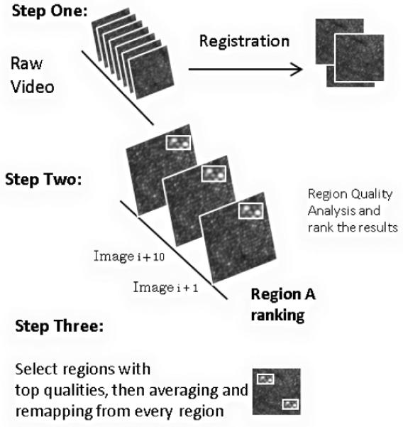
Schematic information flow for lucky averaging

To test this approach, cone photoreceptor images were acquired from different subjects and processed. The AOSLO system has been described previously [4]. The pixel clock was 30MHz, and the frame rate was 30Hz. The AO control loop operated at 15Hz. Each image was 800 by 520 pixels, corresponding to 2.79°×1.78° imaging field in the retina. Each image series consisted of approximately 100 frames acquired sequentially in ~3 second. Once aligned, a window of 9 by 7 pixels was created and swept across the image, pixel-by-pixel to compute an image quality metric. A window of this size represented 450 μs in time and about 70 μm² in space.

While any appropriate image quality metric can be used, for this paper we implemented two examples - a sharpness metric and a gray level co-occurrence matrix (GLCM). The sharpness metric has been used for incoherent imaging in astronomy and synthetic radar image reconstructions [5]. It represents a sum of a nonlinear point transformation of the image and is generally defined as

$$s={\Sigma }_{(x,y)}w(x,y)I{(x,y)}^{\beta }$$ (1)

where x,y are pixel coordinates, and β is the power of the pixel intensity, w(x,y) is the weight for each pixel, and I(x,y) is the pixel intensity.

In practice, we set β as 2, and w(x,y) as 1. Normalization is also considered, as [6] indicates. The metric is finally defined as,

$$S_{(x_0,y_0,index)}=\frac{{\Sigma }_{(x_0-\Delta x\le x\le x_0+\Delta x,y_0-\Delta y\le y\le y_0+\Delta y)}{I}_{index}{(x,y)}^2}{{\left(\Sigma (x_0-\Delta x\le x\le x_0+\Delta x,y_0-\Delta y\le y\le y_0+{\Delta }_y)I_{index}(x,y)\right)}^2}$$ (2)

where x, y are pixel coordinates, x₀ and y₀ represent the coordinates of central pixels of the sampling window. Δx and Δy represent half the sampling window width and height respectively. The index represents the frame index number of the analyzed image within the sequence

The second image metric is GLCM, measuring how often different combinations of gray levels co-occur in an image region [7], computed as in equation (3). For a given Δd which represents pixel separation between a pair of pixels, we compute GLCM_Δd by examining pixel pair along 8 different directions from 0 degree to 315 degree with 45 degree increment, where the element GLCM_Δd (i,j) represents the number of the pixel pair with gray level pair(i,j). The parameter d represents the two dimensional position vector of the pixel in the image. We typically normalize the GLCM by dividing the whole matrix with the sum of all elements in the matrix. Once a GLCM has been constructed, several types of statistical analysis can be performed. Local contrast is one of these measures, taking GLCM as contrast weights, computed as in equation (4), where α is the power of the gray level difference between a pixel pair, and β is the power of GLCM. In practice, for cone photoreceptor images, we calculated GLCM₃ or GLCM₄. α and β are set as 2 and 1 respectively.

$$GLC{M}_{\left(\Delta d\right)}(i,j)={\Sigma }_{d\le AnalyzedRegion}\{\begin{array}{cc}1,\hfill & ifI\left(d\right)=i,I(d+\Delta d)=j\hfill \\ 0,\hfill & otherwise;\hfill \end{array}\phantom{\}}$$ (3)

$$Contrast(\alpha ,\beta )={\Sigma }_i{\Sigma }_j{(i-j)}^{\alpha }GLCM{(i,j)}^{\beta }$$ (4)

The calculation result S(x₀, y_0, frame index) from equation (2) or equation (4) is then assigned to the central pixel (x₀,y₀). A quality metric S(x, y, frame index) is then generated for every pixel in the image sequence.

For either metric the final step is to set a threshold for including a pixel. That is, for a given pixel position(x,y), we can include (for instance) the 30%of the instances within the sequence when those pixel instances have the highest value of the image quality metric. The final image is then the average of those pixels. This is computationally fairly simple, taking about 3 minutes for 100 frames, using a 2.8 GHz PC with 8GB of memory and implemented in MATLAB.

Figure 2 and 3 compare results from the different averaging methods. Similar results were obtained on two other subjects. In single frame images, we observe noise and contrast variance across the image (Fig. 2a). The average image is less noisy(Fig. 2b) and in an enlargement more details can be observed due to the decreased noise(Fig. 3b). However, some cones are dim and some regions are still blurry. For the lucky-averaging (Fig. 2c, 2d and Fig. 3c, 3d), the contrast reduction is decreased. Cones are somewhat brighter and more distinct, suggesting local contrast and resolution improvement. To quantify the difference between lucky averaging and normal averaging, a power spectral analysis was performed. We calculated the power ratio, as a function of frequency between lucky averaging and standard averaging (Fig. 4). Thus, a ratio greater than one indicates a higher spectral power for lucky averaging at a given frequency. The average increase in powers between either lucky averaging imaging metric and standard averaging is 20% and the improvement extends all the way to the optical cut-off frequency which is about 0.4 cycles/pixels based on the system resolution 2.5?m [8] for this subject’s pupil size of 6 mm. Beyond the cut off frequency, the ratio fluctuates around one, indicating that the noise level is close between the two schemes. The two metrics used for lucky averaging produced similar improvements for these images, but because the scheme can be used with most local quality evaluation metrics the approach is general and can be tuned to optimize extraction of the most appropriate information.

Figure 2.

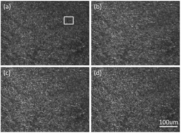
Image Comparison. Each image is 1.39° by 1.17° cropped from original frames. (a) a single-frame image (b) the image with normal averaging scheme, 20% frames are selected. (c) image after lucky averaging top 30% pixels from image sequence, with GLCM contrast metric (d) image after lucky averaging top 30% pixels from image sequence, with sharpness metric

Figure 3.

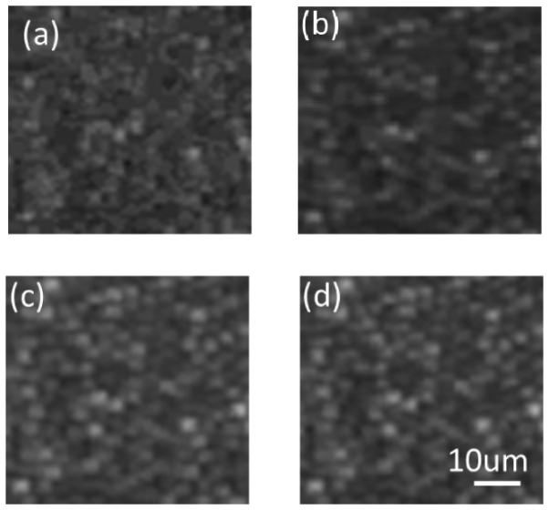
Enlarged regions location indicated in white in figure 2. Fig 3(a-d) correspond to the same region in figure 2(a-d).

Figure 4.

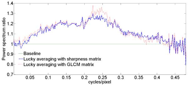
(color online)The spectral power ratio between lucky and conventional averaging. Dotted curve in red: ratio of Fig 3(c) to Fig 3(b); Dashed curve in blue: spectrum ratio of Fig 3(d) to Fig 3(b);

To investigate the role of the criterion for including pixels, we processed the same region in Fig. 3 with varied criteria to include the best 20%, 30% and 40% of pixels using GLCM method (Fig. 5). As expected, the improvement is largest with the lowest percentage criterion; however there is a limit, since as the criterion uses fewer samples, the impact of photon noise increases. Thus, the choice of criterion will be a balance between reducing random noise through averaging and improving contrast by picking the best “moments”. One simple solution to this tradeoff is to collect more data for the same region of interest. It is also possible to base the criterion on the information itself, optimizing S/N ratio.

Figure 5.

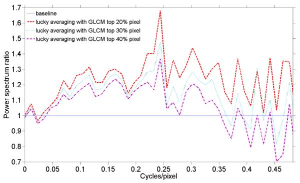
(color online) The spectral power ratios for different inclusion criteria; The baseline was based on conventional averaging. The dash-dot line in purple, the dotted line in light blue and the dashed line in red represent inclusion criteria for the best 20%, 30% and 40% of pixels respectively

In summary, “lucky averaging”, analogous to “lucky imaging”, has been applied to AOSLO image post processing. The image sequence is evaluated based on small regions instead of frames. The quality is enhanced by 20%, suggesting a better use of the data by this processing scheme. A larger dataset is necessary but collecting 3 or 4 seconds worth of data for each retinal region is realistic.