Biological Parametric Mapping Accounting for Random Regressors with Regression Calibration and Model II Regression

Abstract

Massively univariate regression and inference in the form of statistical parametric mapping have transformed the way in which multi-dimensional imaging data are studied. In functional and structural neuroimaging, the de facto standard “design matrix”-based general linear regression model and its multi-level cousins have enabled investigation of the biological basis of the human brain. With modern study designs, it is possible to acquire multi-modal three-dimensional assessments of the same individuals — e.g., structural, functional and quantitative magnetic resonance imaging, alongside functional and ligand binding maps with positron emission tomography. Largely, current statistical methods in the imaging community assume that the regressors are non-random. For more realistic multi-parametric assessment (e.g., voxel-wise modeling), distributional consideration of all observations is appropriate. Herein, we discuss two unified regression and inference approaches, model II regression and regression calibration, for use in massively univariate inference with imaging data. These methods use the design matrix paradigm and account for both random and non-random imaging regressors. We characterize these methods in simulation and illustrate their use on an empirical dataset. Both methods have been made readily available as a toolbox plug-in for the SPM software.

INTRODUCTION

The strong relationship between structure and biological function holds true from the macroscopic scale of multi-cellular organisms to the nano-scale of biomacromolecules. Experience informs the clinical researcher that such structure-function relationships must also exist in the brain and, when discovered and quantified, will be powerful informers for early disease detection, prevention, and our overall understanding of the brain. Brain imaging modalities, such as positron emission tomography (PET) and magnetic resonance imaging (MRI), are primary methods for investigating brain structure and function. Quantification of the structure function relationship using imaging data, however, has been challenging owing to the high-dimensional nature of the data and issues of multiple comparisons.

Statistical Parametric Mapping (SPM) enables exploration of relational hypotheses using the design matrix paradigm (i.e., “y = Xβ”) without a priori assumptions of regions of interest (ROIs) where the correlations would occur (Friston, Frith et al. 1990; Friston, Frith et al. 1991). SPM was initially limited to single modality regression with imaging data represented only in the regressand (i.e., only y varied voxel by voxel) until extensions (e.g., Biological Parametric Mapping, BPM) were developed to enable multi-modality regression (i.e., to allow X to vary voxel by voxel) (Casanova, Srikanth et al. 2007; Oakes, Fox et al. 2007) and provide for inference robust to artifacts (Yang, Beason-Held et al. 2011). These multi-modal methods rely on the traditional ordinary least squares (OLS) approach in which regressors are exactly known (i.e., conditional inference). OLS inference is not inverse consistent; interchanging the regressor and regressand images would yield different estimates of relationships (as reviewed by (Altman 1999)). Although conditional inference may be reasonable in SPM, where scalar regressors are likely to have significantly less variance than the regressand imaging data such an assumption is clearly violated when both regressors and regressand are observations from imaging data (as in BPM).

Regression analysis accounting for errors in regressors would greatly improve the credibility of the BPM model by reasonably considering the randomness of the imaging modality in both the regressors and the regressands. Empirically successful statistical methods accounting for random regressors have been developed including regression calibration (Carroll, Ruppert et al. 2006) and model II regression (York 1966; Ludbrook 2010). The specific contributions of this work are that, (1) we implement these methods (which are established and accepted in statistical community) in the context of neuroimaging, (2) we demonstrate that these approaches are compatible with the design matrix paradigm, contrast-based hypothesis testing, and multiple comparison correction frameworks, and (3) we evaluate application of these methods in simulations and an empirical illustration in the context of multi-modality image regression. Herein, we focus on multi-modality inference; possible extensions to temporal modeling are discussed but left as future work.

Notation

For consistency, we have adopted the following notation. Scalar quantities are represented by italic, lower case symbols (e.g., σ²). Vectors are represented by bold, italic, lower case symbols (e.g., y). Matrices are bold, upper case symbols (e.g., X). The symbol ~ is used to note “distributed as,” with $\mathcal{N}$ used to represent the multivariate Normal distribution. Subscripts are used to indicate context. For example, the subscript “obs” indicates the observed value of a random variable. Superscripts are used with matrices to index columns (i.e.,X⁽ⁱ⁾ is the vector corresponding to the i^th column of X) and with vectors to indicate entries (i.e., β⁽ⁱ⁾ is the i^th element of β). Braces (“{ }”) are used to indicate sets, while “:” is used to indicate vector concatenation and “’” indicates transpose. The hat (^) indicates an estimated value of a random variable.

Theory

Our aim is to explain the observed intensity from one imaging modality, y, with a set of regressors, X, of which at least one member is observed intensity from another imaging modality. We begin with a typical general linear model (GLM) and reformulate it to explicitly reflect the clinical imaging case of both random and non-random regressors. To begin, GLM is formulated as,

$${\mathit{y}}_{\mathit{obs}}=\mathit{y}+{\eta }_y,{\eta }_y\sim \mathcal{N}(0,{\sigma }_y^2\mathbf{I})$$ (1)

$$\mathit{y}=\mathbf{X}\beta +\epsilon ,\epsilon \sim \mathcal{N}(0,{\sigma }_{\epsilon }^2\mathbf{I})$$ (2)

where η_y is a parameterization of observational error in y, β is a vector of the fitted coefficients, ε is the regression error in the model fit, and I is the identity matrix. The observation error (η_y) and the equation (or model error) (ε) are assumed to be mutually independent.

Let us consider the columns of the design matrix, X, in two disjoint sets: fixed regressors whose values are considered to be exactly known, X_f, (i.e., the variance in observed values is much less than the variance of the regressand) and random regressors, X_r, whose observations have non-negligible variance (i.e., X=[X_r:X_f]). Note, β must be correspondingly partitioned into β_f and β_r (i.e.,β = [β_r:β_f]). In BPM, all regressors in the design matrix are treated as fixed regressors, but in fact, the image intensities in the design matrix are observed with measurement error. The use of traditional OLS yields a non-inverse consistent fit, as illustrated in Figure 1, due to the model that only considering measurement errors occur in y, but ignoring the errors in x. If the roles of x and y are exchanged, the estimated coefficients are altered (i.e., the errors are assumed to lie in x and the fit is not inverse consistent).

Figure 1.

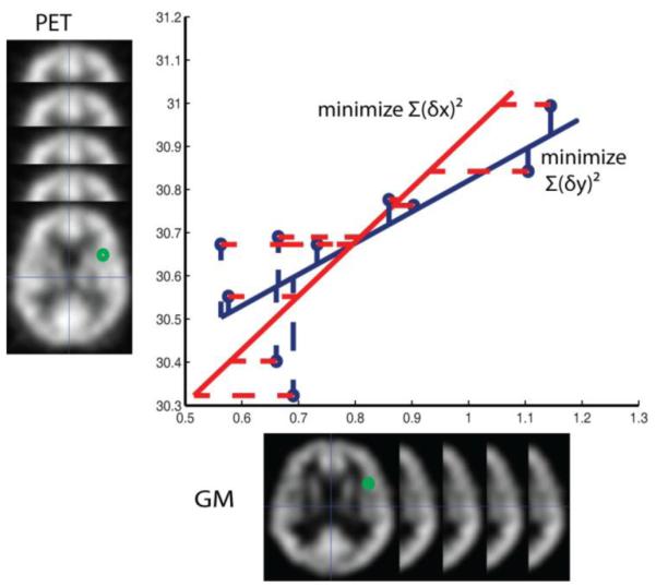
Optimal regression fitting depends on how distance is considered. In traditional OLS (blue: regress “x on y”), the sum of squared vertical distance is minimized (blue dash), while in the reciprocal problem with OLS (red: “y on x”), the sum of squared horizontal distance (red dash) is minimized. The resulting regression lines from the two approaches (solid blue and solid red respectively) disagree with each other. The estimation result depends on in which direction we minimize the distance such that a symmetric optimal model cannot be achieved.

In the more realistic regressor measurement error model, the X_r are not exactly known and instead are estimated from observations, X_r,obs, containing measurement error:

$${\mathbf{X}}_{r,\mathit{obs}}={\mathbf{X}}_r+{\eta }_x,{\eta }_x\sim \mathcal{N}(0,\mathrm{diag}({\sigma }_{x,r}^2\left)\right)$$ (3)

where η_x is zero-mean Gaussian distributed measurement error with variances ${\sigma }_{x,r}^2$. Note diag indicates a matrix with diagonal elements corresponding to the given vector. Herein, we will discuss two methods that, unlike ordinary least squares, can account for the regressor measurement error: regression calibration and model II regression.

Theory: Regression Calibration

Regression calibration is a simple, widely-applicable approach to measurement error analysis described in (Carroll, Ruppert et al. 2006). The random regressors, X_r, are observed multiple times to obtain replicated measurements, X_r,obs1, X_r,obs2,…X_r,obsd for d repeated measurements. To create an estimate of X_r, one could simply average the repeated measurements. However, regression calibration improves upon the average by accounting for the covariance between all regressors (including the fixed regressors). In short, the new estimated values for the random regressors, M_r, are obtained through approximation of E(X_r|X_f,{X_r,obsi}_i=1…d), where E indicates the expected value. Using the new approximation of X_r, a standard analysis on the estimated general linear model is performed,

$${\mathit{y}}_{\mathit{obs}}={\mathbf{M}}_r{\beta }_r+{\mathbf{X}}_f{\beta }_f+\epsilon +{\eta }_y.$$ (4)

For inference on the significance of β estimates, we used the residual bootstrap method as reviewed in (Carroll, Ruppert et al. 2006).

Theory: Model II Regression

In medical image analysis, especially in functional MRI, it is difficult or impossible to obtain replicated measurements for X. Additionally, replicated measurements are complicated by the increased resource requirements, increased cost of experimentation, and increased level of volunteer participation. To work within these constraints and avoid the need for replicated measurements, we consider model II regression. model II theory diverges from OLS through incorporation of the noise in random regressors (as in Eq. 3), and Eq. 2 becomes,

$$\mathit{y}={\mathbf{X}}_r{\beta }_r+{\mathbf{X}}_f{\beta }_f+{\eta }_y$$ (5)

Let z_i be a vector concatenating the observational errors in y⁽ⁱ⁾ and in ${\mathrm{X}}_{r,\mathit{obs}}^{\left(i\right)}$. Note that the observational errors, z_i, are errors across subjects and not conditional errors across an image. Given that each ${\mathrm{X}}_{r,\mathit{obs}}^{\left(i\right)}$ vector is observed from a unique experimental technique, the elements of z_i are independent and that the row vectors z_i are also independent across subjects. Therefore, the errors across z_i follow a multivariate normal distribution (Friston, Holmes et al. 1994):

$${\mathit{z}}_i=\left[{\mathit{y}}_{\mathit{obs}}^{\left(i\right)}-{\mathit{y}}^{\left(i\right)}:X_{r,\mathit{obs}}^{\left(i\right)}-{\mathbf{X}}_r^{\left(i\right)}\right]\sim \mathcal{N}(0,\Sigma ).$$ (6)

Under these assumptions (normal, independent, and identically distributed), the log-likelihood of the observed data, given the model in Eq. 5 and Eq. 6 is,

$$\ln P\left({\mathit{y}}_{\mathit{obs}},{\mathbf{X}}_{r,\mathit{obs}}\mid \beta ,\Sigma ,\mathit{y},{\mathbf{X}}_r\right)=\sum _{i=1}^n\ln \left(2{\pi }^{-n∕2}\left(\det {\left(\Sigma \right)}^{-1∕2}\right)\right)-\frac{1}{2}\sum _{i=1}^n\left({\mathit{z}}_i{\Sigma }^{-1}{\mathit{z}}_i^{\prime }\right)$$ (7)

where there are n subjects (rows of X).

Maximizing the log likelihood, Eq. 7, is equivalent to minimizing $s={\sum }_{i=1}^n\left(z_i{\Sigma }^{-1}{z}_i^{\prime }\right)$. With the assumption of independent observations, the covariance matrix, Σ, is diagonal with entries $[{\sigma }_y^2:{\sigma }_{x,r}^2]$. Hence, s can be re-expressed as,

$$s={\sigma }_y^{-2}{\Vert {\mathit{y}}_{\mathit{obs}}-\mathit{y}\Vert }_{L2}^2+\sum _{j=1}^q{\left({\sigma }_{x,r}^{\left(j\right)}\right)}^{-2}{\Vert {\mathbf{X}}_{r,\mathit{obs}}^{\left(j\right)}-{\mathbf{X}}_r^{\left(j\right)}\Vert }_{L2}^2$$ (8)

where there are q regressor random variables and the subscript L2 indicates the L² norm (i.e., square root of the sum of squares). Eq. 8 is minimized when its partial derivatives with respect to each dependent variable is zero. We first solve for each ${\mathrm{X}}_{r,\mathit{obs}}^{\left(i\right)}$ by differentiating s with respect to ${\mathrm{X}}_{r,\mathit{obs}}^{\left(i\right)}$, setting the result to zero, and using the linear model relation (Eq. 5). Some manipulation yields,

$$s=\frac{{\Vert {\mathit{y}}_{\mathit{obs}}-({\mathbf{X}}_{r,\mathit{obs}}{\beta }_r+{\mathbf{X}}_f{\beta }_f)\Vert }_{L2}^2}{{\sigma }_y^2+{\sigma }_{x,r}^{2\prime }{\beta }_r}$$ (9)

Eq. 9 is now independent of the unknown X_r and provides an intuitive form as the error in the numerator is balanced by the individual variances in the denominator and mirrors the more readily available multivariate case with non-random X and the univariate case that accounts for one random regressor (Press 2007). Eq. 9 is a function of two unknown vectors: β and σ.

Hence, the variance ratios need to be known in order to minimize s by solving β; otherwise the system of equations will be undetermined for σ (Carroll and Ruppert 1996). Note that only the relative variance between observations factors into s (as opposed to the absolute variances). If the ratios for $\frac{{\sigma }_{x,r}^2}{{\sigma }_y^2}$ are known (or can be reasonably estimated), then the optimization becomes well defined with an equal number of unknown to available equations. We employ numeric Nelder–Mead method to optimize with respect to β. If we add the further assumption that the ratio of the overall measurement error ratio across subjects is proportional to the ratio of the image noise variance, then we can estimate the measurement error ratio by estimating the ratio of image noise for each modality. We note that the maximum likelihood estimate of β are asymptotically normally distributed. As reviewed in (Penny, Friston et al. 2006), we can use the Fisher information to construct the asymptotic distribution of contrasts of the parameter estimates (i.e., c’$\widehat{\beta }$) and estimate t-values (and corresponding p-values) for inference.

A common theoretical problem with applications of model II regression is that it is tends to overestimate the influence of the error of the regressors (i.e., η_x and η_y) by ignoring the equation error (∊) (Carroll, Ruppert et al. 2006). Here, we partially address this problem by partitioning the total error in an arbitrary (but reasonably justified) manner according to the relative variances of each measurement (i.e., ${\sigma }_y^2$ versus ${\sigma }_{x,r}^2$). Hemodynamics and/or correlated error models could be addressed in this framework through estimation and pre-whitening as is typically done with restricted maximum likelihood approaches for fMRI time series (Friston, Glaser et al. 2002; Friston, Penny et al. 2002), but secondary noise modeling is beyond the scope of this initial work.

Methods and Results

Regression calibration and model II regression were implemented in MATLAB as an SPM Toolbox and integrated with a cluster processing environment as illustrated in Figure 2. Regression calibration and model II regression are incorporated as regression method choices in the BPM toolbox for the SPM software using Matlab (Mathworks, Natick, MA). These modified software and demonstration data corresponding to the simulation examples are released in open source at http://www.nitrc.org/projects/rbpm/.

Figure 2.

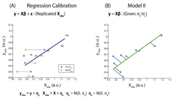
Regression calibration (A) and model II regression (B) address uncertainty in multiple variables. Regression calibration uses repeated measures to estimate variance in the regressors, while model II regression relies on an estimation of the relative variance between the regressors and regressands to minimize error.

Single Voxel Simulations

Regression Calibration vs OLS

For each of the following single voxel simulation scenarios, a simulated voxel with 50 observations (i.e., subjects) was studied using a model with one random regressor, one fixed regressor, and a single constant: y = x_rβ_r + x_fβ_f + β₁ + ε. In each of 500 Monte Carlo trials, regressors (x_r and x_f) were chosen randomly from the uniform distribution [0 1], β_T were chosen randomly from the uniform distribution [0 2], and errors were added to y and x_r from a normal distribution with variances ${\sigma }_y^2$ and ${\sigma }_{x,r}^2$ respectively. Two measurements for each x_r,(x_r,obs1,x_r,obs2) were simulated. OLS was performed using only the first measurement x_r,obs1. Regression calibration was evaluated compared to OLS with the relative root mean squared error (rRMSE) in β (β_rRMSE), defined over each Monte Carlo Simulation (sn) for regression calibration (RC) and OLS estimates relative to the true (T) parameters:

$${\beta }_{\mathit{rRMSE}}=\frac{\sqrt{{\Sigma }_{\mathit{sn}=1}^{500}{\left({\widehat{\beta }}_{\mathit{RC},\mathit{sn}}-{\beta }_{T,\mathit{sn}}\right)}^2}}{\sqrt{{\Sigma }_{\mathit{sn}=1}^{500}{\left({\widehat{\beta }}_{\mathit{OLS},\mathit{sn}}-{\beta }_{T,\mathit{sn}}\right)}^2}}$$ (10)

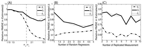
1. Regression calibration vs OLS response to σ_x,r:σ_y ratios (Figure 3A). Simulations were performed varying σ_x,r:σ_y. Regression calibration performs equally well as OLS with small σ_x,r:σ_y, but becomes advantageous as more relative error is introduced into x_r observations. This advantage is most notable in random regressor coefficient β_r.

2. Regression calibration vs OLS response to number of random regressors (Figure 3B). The above model was altered by including up to four additional random regressors with randomized coefficients. Over the model complexity range investigated, regression calibration has universally smaller errors in all estimated coefficients compared to OLS. Interestingly, the advantage of regression calibration over OLS for β_f and β₁ increased with increasing model complexity, while the advantage over OLS decreased for β_r.

3. Regression calibration sensitivity to the number of replicated measurements (Figure 3C). To assess the response of regression calibration to the number of replicated measurements, the number of random regressor measurements was increased from two to ten. For the increasing number of replicated measurements, the accuracy of regression calibration for β_r, β_f, and β₁, is improved slightly over OLS. We note that since the noise on the regressors was Gaussian in this simulation, regression calibration (which assumes a Gaussian error model) was able to accurately model the variance with limited numbers of observations.

Figure 3.

The rRMSE of regression calibration to OLS for each estimated coefficient (β_r,β_f,β₁) are plotted as a function of the ratio of the true standard deviations, σ_x,r:σ_y (A), the number of random regressors, ${\mathrm{X}}_r^{\left(j\right)}$ (B), and the number of replicated measurements (C). (Note, y-axis was visually optimized for each figure and are not common across A, B, and C.) With increasing σ_x,r:σ_y ratios, regression calibration has increased relative accuracy in β_r estimates compared to OLS. The common simulation shared in (A, B, C) is indicated by a gray line.

Model II Regression vs OLS

Model II regression was compared to OLS using a similar model as was used for comparisons with regression calibration. A simple model with one fixed and one random regressor was used y = x_rβ_r + x_fβ_f + β₁. For 50 observations, regressors (x_r and x_f) were chosen randomly from the uniform distribution [0 1], β_T were chosen randomly from the uniform distribution [0 2] and errors were added to y and x_r from a normal distribution with variances ${\sigma }_y^2$ and ${\sigma }_{x,r}^2$, respectively. Model II regression and OLS are performed on the same dataset. Relative performance of model II to OLS is quantified by the rRMSE in β (Eq. 10).

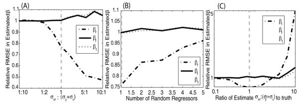
1. Model II vs OLS response to σ_x,r:σ_y ratios (Figure 4A). Simulations were performed varying σ_x,r:σ_y. The performance of model II regression and OLS are comparable for small σ_x,r:σ_y, but model II regression becomes more advantageous as more relative error is introduced into x_r,obs. The improvement is observed specifically on the random regressor coefficient β_r, whereas the constants not associated with random regressors, β₁ and β_f, remain with approximately equal accuracy in estimation between the two models.

2. Model II vs OLS response to number of random regressors (Figure 4B). The above model was altered by including up to four additional random regressors with randomized coefficients (randomly drawn from the uniform distribution [0 2]). Model II has smaller errors in the β_r estimates than OLS; however, model II becomes less advantageous with increases in the number of random regressors. Note that the number of observations was not increased to compensate for the increased model complexity; therefore less data per regressor is available with more regressors.

3. Model II sensitivity to the estimated ratio (Figure 4C). To assess the robustness of model II against varying levels of accuracy in the σ_x,r:σ_y ratio estimates, the estimated ratio of the variance was altered between 1/10th and 10 times its true value, which was set at one. Under the cases simulated here, model II is insensitive to the ratio mis-estimation range 0.5 to 2, and relatively insensitive over the range 0.1 to 3. At extremely incorrect ratio values, the β_r estimate rapidly loses accuracy. Based on this analysis we can apply model II regression using an estimated error ratio, with reasonable confidence in the methods’ tolerance to mis-estimation of variance ratios.

Figure 4.

The rRMSE of model II to OLS for each estimated coefficient (β_r,β_f,β1) are plotted as a function of the ratio of the true standard deviations, σ_x,r:σ_y (A), the number of random regressors, ${\mathrm{X}}_r^{\left(j\right)}$ (B) and the accuracy of the ratio estimate (C). (Note, y-axis were visually optimized for each figure and are not common across A, B, and C.) With increasing σ_x,r:σ_y ratios, model II regression has increased relative accuracy in β_r estimates compared to OLS with increasing σ_x,r:σ_y ratios. In (C), the estimated ratio of σ_x,r:σ_y was allowed to deviate from the simulated value,σ_x,r:σ_y = 1. The common simulation shared in (A, B, C) is indicated by a gray line.

Volumetric Imaging Simulation

To explore the performance of these methods on an imaging dataset, we simulated images of two modalities and regressed one modality on the other modality. The true regressor images are simulated from smoothed gray matter (GM) density images of 40 participants in the normal aging study of the Baltimore Longitudinal Study on Aging (BLSA) neuroimaging project consisting of 79×95×69 voxels with 0.94×0.94×1.5 mm resolution (Resnick, Goldszal et al. 2000). To create repeated measurements for regression calibration, we simulated two observed regressor images for each subject. OLS and model II were applied to the first set of measurements. To test the regression methods, a simple model with a single random regressor and constant was used, y = β_rx_r + β₁ + ε. Inside the caudate region: β_r = 1.5, inside the putamen: β_r = −0.6, and for all other brain regions: β_r = 0. The observed regressand images and the observed regressor images were generated by adding zero mean Gaussian noise across subjects and the standard deviation used for each voxel was chosen to maintain an SNR around 15 for each image (SNR is defined as the mean signal divided by the standard deviation of noise).

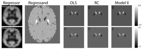
Figure 5 presents the simulated images, the ${\widehat{\beta }}_r$ from each method, and the t-map for the regressor images (the spatial map of the test statistic for the null hypothesis). For clarity, the number of replicated measurements used for regression calibration was two and the estimated and true ratio for σ_x,r:σ_y was one for model II regression. The simulation method was repeated 10 times to create 10 imaging datasets (each of the 10 imaging datasets contained 40 × 2 x_r images and 40 y images). The average false positive rate (FPR), average false negative rate (FNR), and the root mean square error are calculated using the uncorrected p-value < 0.001. The results are summarized in Table 1.

Figure 5.

Simulated imaging associations. The first column shows two noisy regressor images for one subject, the first measurement is used in OLS regression and model II regression while both of them are used in regression calibration. The second column shows the paired noisy regressand image. The estimated coefficient β map and the positive t-map are displayed in the upper right-hand row of and lower left-hand row respectively. The β and t-maps are shown for OLS, regression calibration (RC) and model II regression. The differences between the methods are difficult to appreciate in a visual comparison; please see Table 1 for a quantitative summary.

Table 1.

Comparison of methods based on simulated imaging data

	Outside (β=0)		Inside Caudate (β=1.5)		Inside Putamen (β=−0.6)
	FPR (%)	RMSE	FNR (%)	RMSE	FNR (%)	RMSE
OLS	0.1±0.008	0.05±0.0001	0	0.24±0.003	1.7±0.2	0.12 ±0.0015
RC	0.1± 0.006	0.06±0.008	0.04±0.05	0.11±0.002	1.5±0.2	0.08± 0.001
Model II	0.07± 0.006	0.06±0.002	0	0.13±0.004	0.2±0.09	0.09± 0.001

The significance is calculated according to an uncorrected p-value, p<0.001.

In this simple model, both OLS and regression calibration control the type I error rate as expected (FP, Table 1). Meanwhile, regression calibration and model II regression improve the true positive rate as compared to OLS regression (100-FNR, Table 1). For the root mean square error, when the true coefficient is zero (β_r = 0), the OLS method slightly outperforms the regression calibration and model II regression; when the relationship between x_r and y exists (β_r ≠ 0), both regression calibration and model II regression outperform OLS. Regression calibration is slightly superior to model II regression (but requires additional measurements).

Empirical demonstration of model II regression

Image-on-image regression offers a direct opportunity to study associations between differing spatially located factors. As an illustrative example, consider potential correlations between gray matter (GM) tissue density (a structural measure) and PET signal (a measure of functional activity). A first model would associate tissue presence with greater functional signal. An analysis of modulating factors for this relationship (such as disease condition, intervention, or task) could reveal anatomical correlates of functional reorganization and shed light on the applicability of the structural-functional hypothesis.

Following this approach, we perform regression analysis of the relationship between anatomical MRI GM images and functional PET images. We used a sub-cohort of 23 healthy participants (14 M/9 F, 60-85 y/o at baseline). Each subject was studied annually for eight years with a T1-weighted MRI sequence (1.5T, GE Medical Systems, SPGR, 0.9375×0.9375×1.5 mm, 256×256×124 mm field of view) and PET data (GE 4096+ scanner, 15 slices of 6.5mm thickness, 60s). The baseline scan was denoted as year 1 and the last scan was denoted as year 9. The data were preprocessed with SPM5 (http://www.fil.ion.ucl.ac.uk/spm/software/spm5). The structural scans were normalized to MNI-space, segmented and smoothed (12 mm Gaussian kernel) to obtain smooth GM density images. PET images were normalized, smoothed (12 mm Gaussian kernel) to MNI-space, and calibrated for global blood flow measurements to form cerebral blood for measurements and normalized to [0 1] scalar.

Regression was performed in both directions in order to quantify both structure→function and function→structure relationships. The “structure” data was constructed by concatenating all smoothed gray matter data for year 1 and year 9 and all subjects, and the “function” data was constructed by concatenating all corresponding, smoothed, calibrated PET images. Hence, the regression model used one random regressor and one single constant. Note that this analysis is simplified to illustrate the use of these methods; a traditional application would also include confounds (age, gender, pre-existing conditions, year of scan, etc.) and an analysis of time courses and interaction terms. An extended characterization of the BLSA data is ongoing and beyond the scope of this work demonstrating statistical methods.

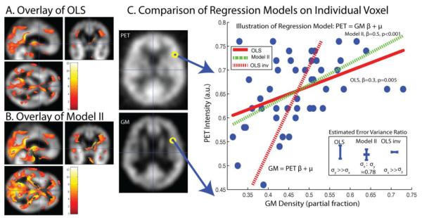
As is common in practice, only one measurement for each modality image is available and regression calibration cannot be applied. The model II σ_x,r:σ_y ratio is estimated following the method in (Rajan, Poot et al. 2010), with the window size for the method selected according to the image modality. The raw data and the resulting OLS and model II regression lines for a single voxel comparison are displayed in Figure 6. The model II regression model is symmetric, i.e., the mapping PET→GM is the inverse of the mapping GM → PET while OLS is not. The corresponding estimated variances for model II are also smaller than the corresponding estimated variances in OLS forward regression and OLS inverse regression.

Figure 6.

Model II and OLS multi-modality regression analysis. OLS (A) and Model II (B) lead to distinct patterns of significant differences (p<0.001, uncorrected) when applied to identical empirical datasets and association models. Inspection of single voxel: PET vs Grey Matter MRI (GM) illustrates the reasons for the different findings (C). The GLM model used for the forward mapping is y = x_rβ_r + β₁, where y represents PET image intensities and represents GM normalized image intensities. On the left-hand side of (C), example images of PET and GM are shown, along with the location of the single example voxel whose regression analysis is displayed in the right-hand plot. The individual data points (blue circles) were fit using OLS (red lines) and model II regression (green dashed line). Note that the inverse mapping for OLS (red dash) is not the same as the forward mapping (red solid line). The model II mapping was found to be reversible and can be represented by the same line. Resulting error bars and corresponding σ_x,r:σ_y value estimates are compared between OLS and model II in the lower right-hand insert.

Conclusions

Properly accounting for error is essential for valid parameter estimation and statistical inference. Herein, we have demonstrated that a consideration of observation variability is feasible within the confines of a design matrix paradigm. Furthermore, we can readily consider simultaneous treatment of parameters with measurement error alongside traditionally defined fixed parameters. Our formulation of “random observations” remains within the context of a “fixed effects” model as the β_r are deterministic parameters, as opposed to the classic “random effects” model where parameters are stochastic. These two approaches are complementary and could be combined for an appropriate experimental framework. Extension of the random regressor concept to time series, hierarchical, and other complex model designs is a fascinating area for continuing research.

We have observed substantial improvements in model fit using regression calibration and model II regression as opposed to OLS (Figure 3A, Figure 4A). While performance of regression calibration and model II were robust to increasing model complexity (Figure 3B, Figure 4B) and prior estimation of observation variability (applicable to model II only, Figure 4C), the improvements were not universal. When the OLS is appropriate (i.e., ${\sigma }_x^2⪡{\sigma }_y^2$), OLS performs comparable to regression calibration (Figure 3A) and for model II there was a slight increase in observed error relative to OLS (Figure 4A); however, as the relative variance in x_r increased, the OLS assumption of fixed regressors becomes increasingly violated and increased variance could be observed in the OLS estimates. We emphasize that the simulations neglect the many of nuances of empirical studies (e.g., correlations among regressors); these results should be viewed as guide to when alternative regression approaches should be evaluated as opposed to definitive evidence that a particular method is best suited.

On average, differences between the advanced statistical methods and OLS may be subtle as seen in the parameter estimates and statistical maps in Figures 5 and 6. As Table 1 highlights, OLS appears quite robust against false positives; however, this may come at the expensive of reduced power and accuracy. In practice, it is important to consider the impact of the inference approach on individual voxels, as local findings drive interpretation and consideration of the multiple sources of measurement error may lead to different parameters estimates and/or different significance values. Model II and regression calibration can be further adapted to accommodate diverse regression scenarios. For example, a non-parametric method would be more suitable when the distribution assumptions are unknown (Nichols and Holmes 2002) while robust regression methods could be applied in the case of outliers (Huber, Ronchetti et al. 1981; Diedrichsen and Shadmehr 2005; Yang, Beason-Held et al. 2011).

Important areas for further development of model II and regression calibration remain. For parametric regression, other error models besides Gaussian may be more appropriate for specific imaging modalities and warrant further consideration. For model II, interpreting the ratio of model variances is a subject of active consideration as one must consider the potential impact of both the imaging variability and model fit error in multiple dimensions. As discussed, we currently approximate this combined quantity as proportional to the imaging variability alone. Developing methods to relax this assumption would greatly aid in generalization of this approached.

Our presentation of model II regression herein is inverse consistent, provides a logical framework for exploring relationships in multi-modal image analysis, and can help model relative uncertainty in imaging methods. Regression calibration accounts for measurement error and has been shown to improve on OLS in massively-univariate imaging scenarios. The requirement of repeated measurements for regression calibration makes model II a more likely choice for imaging data where repeat scans are uncommon. These methods are readily available in open source as plug-ins for the SPM package. Sample datasets and program documentation are available with the program for download.

References

- Altman DG. Practical statistics for medical research. Chapman & Hall/CRC; Boca Raton, Fla.: 1999. [Google Scholar]
- Carroll R, Ruppert D. The Use and Misuse of Orthogonal Regression in Linear Errors-in-Variables Models. The American Statistician. 1996;50(1) [Google Scholar]
- Carroll RJ, Ruppert D, et al. Measurement error in nonlinear models: a modern perspective. CRC Press; 2006. [Google Scholar]
- Casanova R, Srikanth R, et al. Biological parametric mapping: a statistical toolbox for multimodality brain image analysis. NeuroImage. 2007;34(1):137–143. doi: 10.1016/j.neuroimage.2006.09.011. [DOI] [PMC free article] [PubMed] [Google Scholar]
- Diedrichsen J, Shadmehr R. Detecting and adjusting for artifacts in fMRI time series data. Neuroimage. 2005;27(3):624–634. doi: 10.1016/j.neuroimage.2005.04.039. [DOI] [PMC free article] [PubMed] [Google Scholar]
- Friston K, Frith C, et al. The relationship between global and local changes in PET scans. Journal of Cerebral Blood Flow & Metabolism. 1990;10(4):458–466. doi: 10.1038/jcbfm.1990.88. [DOI] [PubMed] [Google Scholar]
- Friston K, Holmes A, et al. Statistical parametric maps in functional imaging: a general linear approach. Human brain mapping. 1994;2(4):189–210. [Google Scholar]
- Friston KJ, Frith C, et al. Comparing functional (PET) images: the assessment of significant change. Journal of Cerebral Blood Flow & Metabolism. 1991;11(4):690–699. doi: 10.1038/jcbfm.1991.122. [DOI] [PubMed] [Google Scholar]
- Friston KJ, Glaser DE, et al. Classical and Bayesian inference in neuroimaging: applications. NeuroImage. 2002;16(2):484–512. doi: 10.1006/nimg.2002.1091. [DOI] [PubMed] [Google Scholar]
- Friston KJ, Penny W, et al. Classical and Bayesian inference in neuroimaging: theory. NeuroImage. 2002;16(2):465–483. doi: 10.1006/nimg.2002.1090. [DOI] [PubMed] [Google Scholar]
- Huber PJ, Ronchetti E, et al. Robust statistics. Wiley Online Library; 1981. [Google Scholar]
- Ludbrook J. Linear regression analysis for comparing two measurers or methods of measurement: But which regression? Clinical and Experimental Pharmacology and Physiology. 2010;37(7):692–699. doi: 10.1111/j.1440-1681.2010.05376.x. [DOI] [PubMed] [Google Scholar]
- Nichols TE, Holmes AP. Nonparametric permutation tests for functional neuroimaging: a primer with examples. Human brain mapping. 2002;15(1):1–25. doi: 10.1002/hbm.1058. [DOI] [PMC free article] [PubMed] [Google Scholar]
- Oakes TR, Fox AS, et al. Integrating VBM into the General Linear Model with voxelwise anatomical covariates. Neuroimage. 2007;34(2):500–508. doi: 10.1016/j.neuroimage.2006.10.007. [DOI] [PMC free article] [PubMed] [Google Scholar]
- Penny WD, Friston KJ, et al., editors. Statistical Parametric Mapping: The Analysis of Functional Brain Images. Academic Press; New York, NY: 2006. [Google Scholar]
- Press W. Numerical recipes: the art of scientific computing. Cambridge Univ Pr.; 2007. [Google Scholar]
- Rajan J, Poot D, et al. Noise measurement from magnitude MRI using local estimates of variance and skewness. Physics in Medicine and Biology. 2010;55:N441. doi: 10.1088/0031-9155/55/16/N02. [DOI] [PubMed] [Google Scholar]
- Resnick SM, Goldszal AF, et al. One-year age changes in MRI brain volumes in older adults. Cerebral Cortex. 2000;10(5):464. doi: 10.1093/cercor/10.5.464. [DOI] [PubMed] [Google Scholar]
- Yang X, Beason-Held L, et al. Biological parametric mapping with robust and non-parametric statistics. Neuroimage. 2011;57(2):423–430. doi: 10.1016/j.neuroimage.2011.04.046. [DOI] [PMC free article] [PubMed] [Google Scholar]
- York D. Least-squares fitting of a straight line: Canadian Jour. Ph. sics. 1966;44:1079–1086. [Google Scholar]
Associated Data
This section collects any data citations, data availability statements, or supplementary materials included in this article.