A quantitative structure–activity relationship (QSAR) study on glycan array data to determine the specificities of glycan-binding proteins

Abstract

Advances in glycan array technology have provided opportunities to automatically and systematically characterize the binding specificities of glycan-binding proteins. However, there is still a lack of robust methods for such analyses. In this study, we developed a novel quantitative structure–activity relationship (QSAR) method to analyze glycan array data. We first decomposed glycan chains into mono-, di-, tri- or tetrasaccharide subtrees. The bond information was incorporated into subtrees to help distinguish glycan chain structures. Then, we performed partial least-squares (PLS) regression on glycan array data using the subtrees as features. The application of QSAR to the glycan array data of different glycan-binding proteins demonstrated that PLS regression using subtree features can obtain higher R² values and a higher percentage of variance explained in glycan array intensities. Based on the regression coefficients of PLS, we were able to effectively identify subtrees that indicate the binding specificities of a glycan-binding protein. Our approach will facilitate the glycan-binding specificity analysis using the glycan array. A user-friendly web tool of the QSAR method is available at http://bci.clemson.edu/tools/glycan_array.

Introduction

Glycan-binding proteins play critical roles in many physiological and pathological processes (Varki 1999), such as inflammation and cancer (Dube and Bertozzi 2005; Fuster and Esko 2005; Lau and Dennis 2008), growth and development (Dennis et al. 1999; Perrimon and Bernfield 2000; Lin 2004) and microbial pathogenesis (Alkhalil et al. 2000; Liu et al. 2002; Stevens et al. 2006; Chandrasekaran et al. 2008). In order to understand the biology of glycan-binding proteins, it is essential to identify their glycan-binding specificities. Recently, the glycan array technology (Drickamer and Taylor 2002; Blixt et al. 2004; Taylor and Drickamer 2009; Wu et al. 2009) provided a high-throughput method to simultaneously measure the binding levels of a certain glycan-binding protein to a large number of glycan molecules. The newest version (V5.0) of the glycan array from the Consortium for Functional Glycomics (CFG; Blixt et al. 2004) contains 611 glycan chains. Currently, large amounts of glycan array data are freely available on the CFG website, and this number is still increasing. These glycan array data have opened up opportunities to discern the binding specificities for glycan-binding proteins.

The glycan array data usually are very complex, and simple visual inspections may not be able to identify the binding specificities of glycan-binding proteins. This poses a great challenge to extract binding specificities of glycan-binding proteins from glycan array data (Porter et al. 2010). Recently, Porter et al. (2010) proposed motif-based methods to discern the substructures that contribute to the binding intensities of the glycan array to a specific glycan-binding protein. Porter et al. manually generated a list of 63 motifs that are substructures of glycan chains identified previously by biological experiments. By comparing the enrichment of those motifs in high- and low-intensity data (intensity segregation) or by statistical testing between glycan data with a certain motif and those without a certain motif (motif segregation), Porter et al. (2010) were able to find motifs that represent binding specificities. However, such predefined motifs may not be sufficient to identify all glycan-binding specificities.

We have developed a novel quantitative structure–activity relationship (QSAR) method to analyze glycan array data. First, we automatically generated different size subtrees from glycan chains as our features. Then, we established the relationship between subtree features and glycan array data using partial least-squares (PLS) regression. We demonstrated our QSAR method on the glycan array data of different glycan-binding proteins. We were able to identify subtrees that represent the glycan-binding specificities of glycan-binding proteins using the regression coefficients of PLS regression. We also showed that the subtree features may be better representations of the glycan-binding specificity than the motifs defined by Porter et al. (2010) are. Furthermore, we developed a user-friendly web tool to facilitate the rapid and automatic analysis of glycan array data. A complete description of our results and methods is given in the sections below.

Results

Coding glycans using subtree features

Glycan chains consist of different kinds of saccharides, such as glucose (Glc), galactose (Gal), mannose (Man), fucose (Fuc), N-acetylglucosamine (GlcNAc) and N-acetylgalactosamine (GalNAc). The structure of a glycan chain can be represented as a rooted tree. Figure 1 shows an example glycan chain that consists of five different saccharides. The binding specificity of a glycan chain to glycan-binding protein usually relies only on its substructures (Chandrasekaran et al. 2008; Porter et al. 2010). In order to capture the structure characteristics of the glycan chain, we parsed the glycan tree into four sets of subtrees (Kuboyama et al. 2006; Yamanishi et al. 2007), each of which has mono-, di-, tri-, or tetrasaccharide subtrees, respectively. Figure 2 shows that the example glycan chain depicted in Figure 1 has been decomposed into five monosaccharide subtrees, five disaccharide subtrees, five trisaccharide subtrees and four tetrasaccharide subtrees, respectively. For each version of the glycan array from the CFG (Blixt et al. 2004), we generated four sets of subtrees for the glycan on the array, including mono-, di-, tri- and tetrasaccharide subtree sets. For example, the CFG glycan array version 2.0 contains 264 glycan chains. We obtained 112 monosaccharide subtrees, 280 disaccharide subtrees, 385 trisaccharide subtrees and 318 tetrasaccharide subtrees from those 264 glycan chains. The four sets of subtrees for the CFG glycan array version 2.0 are listed in Supplementary data, Tables SI–SIV.

Fig. 1.

An example of the glycan chain and its structure. The Sp denotes the spacer arm attached to array.

Fig. 2.

An example of decomposing the glycan chain in Figure 1 into different subtrees. The N indicates the number of saccharide in each subtree.

In order to represent better the substructural characteristics, we included also the bond information in the subtrees. For each saccharide, we included the positions of its bond connections in its representation. Different monosaccharide subtrees will be generated if the same saccharide has different bond connections. For example, we had five monosaccharide subtrees for Gal: (2, 3Galβ); (2, 3Galβ1); (2, 4Galβ1); (2Galβ) and (2Galβ1) from the glycan chains of CFG version 2.0 array. Furthermore, the disaccharides are also represented differently if the bonds between the same pair of saccharides are different. For example, we had two disaccharide subtrees between GlcNAc and Gal: (3,4GlcNAcβ1-3Galβ1) and (3,4GlcNAcβ1-4Galβ1). With the bond information, the subtrees extracted from glycan chains can help distinguish the glycan chains structurally to a certain extent.

After obtaining the subtrees, we used them as features to code the structures of glycan chains on the glycan array. This new coding system has an advantage over the motif-based approach in which the subtree features are more precise and more flexible. Many substructures potentially cannot be represented well in motif-based features since there have been only 63 defined motif features (Porter et al. 2010). On the other hand, the number of subtree features in our method can be much larger (e.g. 112 monosaccharide subtrees, 280 disaccharide subtrees, 385 trisaccharide subtrees and 318 tetrasaccharide subtrees for the CFG glycan array version 2.0). Our method requires more computation than the motif-based method, but this fact shall not be considered as a significant limitation of our method.

For each glycan chain in a certain version of the CFG glycan array, we coded one vector based on each set of mono-, di-, tri- or tetrasaccharide subtrees. The elements in each vector were 1 and 0. If a glycan chain contains a subtree, we coded the feature with 1; otherwise, we coded the feature with 0. Then, feature vectors were used for PLS regression study. A Java program was implemented to automatically parse the glycan chains into mono-, di-, tri- or tetrasaccharide subtrees, and then code the glycan chains with different subtrees.

PLS regression on glycan array data using different features

We first applied the PLS regression to the glycan array data of three plant lectins: Concanavalin A (ConA), Vicia villosa lectin (VVL) and wheat germ agglutinin (WGA), which were also studied by motif-based methods (Porter et al. 2010). The binding specificities of ConA and VVL are relatively simple (Supplementary data 1 and 2). A visual inspection may help to identify some common features from the data. For example, it is shown clearly from the data that ConA binds to the glycans that contain terminal GlcNAc (Supplementary data 1). On the other hand, the binding specificity of WGA is broad and cannot be determined easily by visual examination (Supplementary data 3). To understand how different substructures contribute to binding specificity, we performed PLS regression studies on the glycan array data of those three plant lectins using the mono-, di-, tri- and tetrasaccharide subtree features as well as the motif features of Porter et al. (2010). We first examined the percentage of variances of binding intensities that can be explained using PLS regression models. The percentage of variance explained measures the amount of variation in the given data that a regression model accounts for and it can be used to indicate how well the regression model is. The higher the percentage of variance explained is, the better the PLS regressions perform and the better the subtree features are. Figure 3 plots the percentage of variance explained in the binding intensities of three plant lectins against the number of latent variables (components) in PLS regression. The number of components is automatically determined by their contributions to the variance (see Methods section for more details). Thus, the number of components varied for PLS regressions using different features. Figure 3 shows that the PLS regression using disaccharide subtrees achieved the highest percentage of variance explained for all three glycan array data. The PLS regression using monosaccharide subtrees achieved high percentage of variance explained in the glycan array of ConA and the PLS regression using trisaccharide subtrees achieved high percentage of variance explained in the glycan array of WGA. The PLS regression using a tetrasaccharide subtree and motif features did not obtain high percentage of variance explained in all three glycan array data. Thus, the tetrasaccharide subtree and motif features cannot fully capture the intensity variations in those glycan array data. These results implied that the motif-based method may not have sufficient sensitivity to cover all binding specific substructures.

Fig. 3.

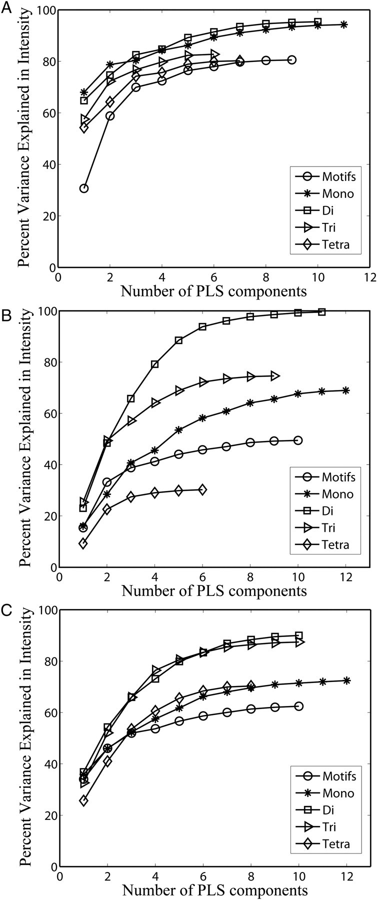
Plot of the percentage of variance explained in the binding intensities of the glycan array data of three plant lectins against the number of components in PLS. Four subtree features and the motif features of Porter et al. (2010) are used for PLS regression. (A) ConA, (B) VVL and (C) WGA.

Then, we calculated the R² statistics of PLS regressions. The R² is a statistical measurement indicating how well a regression approximates real data. The R² analysis (Table I) is consistent with these results of variance explained in the previous paragraph. For ConA, the PLS regressions with all five features can obtain an R² > 0.8. For VVL, only the PLS regression using disaccharide subtrees as features can obtain a significant high R² = 0.9955. For WGA, the PLS regression using both di- and trisaccharide subtrees can obtain high R² > 0.8. Those results confirmed that disaccharide subtrees are good features for characterizing the glycan array data of three plant lectins. We also tested the PLS regression using disaccharide subtrees on the glycan array data of more than 50 plant lectins (Supplementary data, Table SV). We obtained good results (R² > 0.8) on most of the glycan array data except two of them, which have good regression results using trisaccharide subtrees as features. To further examine the results of PLS regressions, we plotted the observed intensities against the fitted intensities calculated by PLS regression using disaccharide subtrees for all three plant lectins. As shown in Figure 4, there are good correlations between the observed intensities and fitted intensities for ConA, VVL and WGA. The dots in Figure 4C are distributed more widely than those in Figure 4A and B, which is consistent with relatively a low R² value obtained by the PLS regression on the glycan array data of WGA. Those plots implied that the disaccharide subtrees can represent the binding specificity of ConA, VVL and WGA well.

Table I.

The R² of PLS regressions on the glycan array data of different glycan-binding proteins using different features

	Motifs	Mono	Di	Tri	Tetra
ConA	0.8052	0.9428	0.9539	0.8276	0.8021
VVL	0.4943	0.6893	0.9955	0.7461	0.3024
WGA	0.6242	0.7132	0.9002	0.8742	0.7027
Peanut agglutinin	0.7774	0.5752	0.9603	0.9966	0.7619
Sambucus nigra lectin	0.6760	0.7871	0.9085	0.7431	0.6509
Dendritic cell-specific ICAM-3 grabbing non-integrin	0.4190	0.5490	0.9179	0.9533	0.8521
Sialic acid-binding immunoglobulin-like lectin 8	N/A	0.9882	0.9927	0.9969	0.9949
CSLEX1 (human CD15s antibody)	N/A	0.3954	0.6362	0.983	0.9952
Sialyl lewisx antibody-10	N/A	0.1374	0.5147	0.9463	0.9949

The highest values of R² are in bold.

Fig. 4.

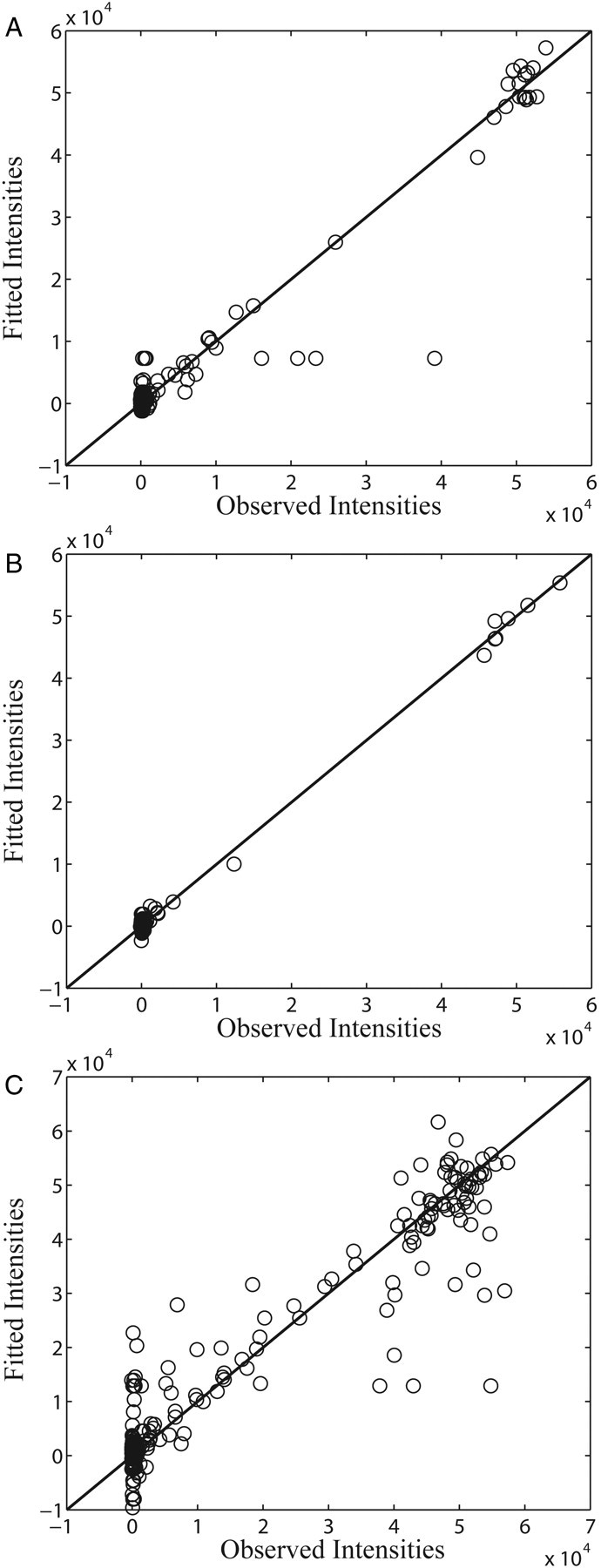
Plot of observed intensities against the fitted intensities calculated by PLS regression using disaccharide subtrees as features. The black lines indicate the line of y = x. (A) ConA, (B) VVL and (C) WGA.

Identification of significant structural features in glycans

We applied the PLS-β method (see Methods section for more details) to identify significant subtrees from the PLS regressions of glycan array data. Tables II–IV list the significant disaccharide subtrees binding to three plant lectins. A significant positive coefficient value indicates the corresponding subtrees have high binding intensities, whereas a negative coefficient value suggests the existence of the subtree feature will reduce the binding intensity. A negative co-efficient value can be achieved when two glycan chains contain the same subtree structure, one with high binding intensity and the other with low binding intensity. For ConA, we identified nine disaccharide subtrees, which cover all 19 glycan chains (Table II) with high binding intensities. Among these nine disaccharide subtrees, α-linked Man is involved in seven and four of these α-linked Mans locate at terminal. Both motif and intensity segregation methods (Porter et al. 2010) ranked the “terminal Manα” as a significant motif. The QSAR results showed internal α-linked Man may also contribute to the binding specificity of ConA as four of our significant disaccharides contained internal α-linked Man. The QSAR method identified that a disaccharide: 3,6Manβ1-4GlcNAcβ1, contributed to binding of 10 glycan chains in CFG glycan array version 2.0:

• 50 (Manα1-3(Manα1-6)Manβ1-4GlcNAcβ1-4GlcNAcβ-Gly)

• 51 (GlcNAcβ1-2Manα1-3(GlcNAcβ1-2Manα1-6)Manβ1-4GlcNAcβ1-4GlcNAcβ-Gly)

• 52 (Galβ1-4GlcNAcβ1-2Manα1-3(Galβ1-4GlcNAcβ1-2Manα1-6)Manβ1-4GlcNAcβ1-4GlcNAcβ-Gly)

• 53 (Neu5Acα2-6Galβ1-4GlcNAcβ1-2Manα1-3(Neu5A cα2-6Galβ1-4GlcNAcβ1-2Manα1-6)Manβ1-4GlcNAcβ1-4GlcNAcβ-Gly)

• 54 (Neu5Acα2-6Galβ1-4GlcNAcβ1-2Manα1-3(Neu5Ac α2-6Galβ1-4GlcNAcβ1-2Manα1-6)Manβ1-4GlcNAcβ1-4GlcNAcβ-Sp8)

• 192 (Manα1-6(Manα1-2Manα1-3)Manα1-6(Manα1-2Manα1-3)Manβ1-4GlcNAcβ1-4GlcNAcβ-Asn), 193 (Manα1-2Manα1-6(Manα1-3)Manα1-6(Manα1-2Manα1-2Manα1-3)Manβ1-4GlcNAcβ1-4GlcNAcβ-Asn)

• 194 (Manα1-2Manα1-2Manα1-3(Manα1-2Manα1-3(Man α1-2Manα1-6)Manα1-6)Manβ1-4GlcNAcβ1-4GlcNAcβ-Asn)

• 197 (Manα1-6(Manα1-3)Manα1-6(Manα1-2Manα1-3)Manβ1-4GlcNAcβ1-4GlcNAcβ-Asn)

• 198 (Manα1-6(Manα1-3)Manα1-6(Manα1-3)Manβ1-4GlcNAcβ1-4GlcNAcβ-Asn)

Table II.

The significant disaccharide subtrees binding specifically to ConA

Disaccharide	Regression coefficient	Glycan numbers
Man5-Asn	46,769.84	199
α-D-Man-Sp8	46,010.46	9
3,6Manα-Sp9	24,403.98	190, 195, 196
Glcα1-4Glcβ	20,758.13	177
3,6Manβ1-4GlcNAcβ1	18,295.47	50, 51, 52, 53, 54, 192, 193, 194, 197, 198
2Manα1-3Manα	17,959.44	189, 191
3Manα-Sp9	17,959.44	189, 191
Manα1-3,6Manα	16,141.64	195, 196
Manα1-3,6Manβ1	10,828.64	50, 198

The subtrees are ordered in descending of coefficients from up to bottom. The numbers of glycan chains including the significant disaccharide in CFG glycan array V2.0 are listed. The regression coefficients are obtained by PLS regression using disaccharide subtrees as features. The glycan numbers are the numbers of glycan chains in CFG glycan array V2.0.

Table IV.

The significant disaccharide subtrees binding specifically to WGA

Disaccharide	Regression coefficient	Glycan numbers
GalNAcα1-3Galβ	42,672.23	86
(6OSO3)GlcNAcβ-Sp8	38,904.61	47
GlcNAcβ1-4MDPLys	36,691.11	168
GalNAcβ1-3,4GlcNAcβ	35,613.5	91
GlcNAcβ1-3,6GlcNAcα	34,575.78	121, 159
β-GlcNAc-Sp0	33,127.88	21
GalNAcα1-2,3Galβ	32,604.2	84
GlcNAcβ1-6Galβ1	31,649.8	176
α-GalNAc-Sp8	31,345.39	10
β-GlcNAc-Sp8	30,441.15	22
GalNAcβ1-4GlcNAcβ	29,082.38	92, 93
GlcNAcα1-6Galβ1	27,593.5	157
2,3Galβ1-4GlcNAcβ	27,091.45	81, 82, 97, 141, 142
Galβ1-4GlcNAcβ	26,658.48	152, 153
2Galβ1-4GlcNAcβ1	26,061.04	60, 70
GlcNAcβ1-3Galβ1	24,471.77	163, 164, 165, 166, 167
Fucα1-4GlcNAcβ	−24,945.3	77
Galα1-4GlcNAcβ	−25,069.7	112
(6OSO3)Galβ1-4GlcNAcβ	−25,093.5	44
KDNa2-3Galβ1	−25,176.4	187, 188

The subtrees are ordered in descending of coefficients from up to bottom. The numbers of glycan chains including the significant disaccharide in CFG glycan array V2.0 are listed. The regression coefficients are obtained by PLS regression using disaccharide subtrees as features. The glycan numbers are the numbers of glycan chains in CFG glycan array V2.0.

This disaccharide is a subset of both “N-glycan high Man” and “N-Glycan complex” that are identified as significant motifs by both motif and intensity segregation methods (Porter et al. 2010). The “N-glycan high Man” motif is defined by Porter et al. (2010) as “a glycan chain with a Manα1-3(Manα1-6(Manα1-3)Manα1-6)Manβ1-4GlcNAcβ1-4GlcNAcβ base” and the “N-glycan complex” is defined as “a glycan chain with a GlcNAcβ1-2Manα1-3(GlcNAcβ1-2Manα1-6)Manβ1-4GlcNAcβ1-4GlcNAcβ base” In CFG glycan array version 2.0, the “N-glycan high Man” motif exists in five glycan chains: 192, 193, 194, 197 and 198 and the “N-glycan complex” motif also exists in five glycan chains: 51, 52, 53, 54 and 201 (Porter et al. 2010). The glycan chain 201 (Neu5Acα2-3(Galβ1-3GalNAcβ1-4)Galβ1-4Glcβ-Sp0) does not contain the disaccharide 3,6Manβ1-4GlcNAcβ1 and its binding intensity with ConA is low. We then performed similar motif segregation study to compare the disaccharide 3,6Manβ1-4GlcNAcβ1 with the “N-glycan high Man” and “N-glycan complex” motifs. We used the two-tail unpaired t-test. The P-values are 2.45E−21 for the “N-glycan high Man” and 1.18E−15 for the “N-glycan complex” without counting glycan chain 201. On the other hand, the P-value for 3,6Manβ1-4GlcNAcβ1 is 4.61E−33. Thus, the disaccharide 3,6Manβ1-4GlcNAcβ1 may be a better representation of the binding specificity of those 10 glycan chains. We also identified a significant disaccharide, Glcα1-4Glcβ, which corresponds to the terminal Glc motifs identified by motif-based methods (Porter et al. 2010). Furthermore, the listing of glycan chains that contain the significant disaccharide in Table II shows that some of those significant disaccharides are dependent of each other. For example, 2Manα1-3Manα and 3Manα-Sp9 both exist in glycan chains 189 (Manα1-2Manα1-2Manα1-3Manα-Sp9) and 191 (Manα1 -2Manα1-3Manα-Sp9). We may be able to merge them as a trisaccharide: 2Manα1-3Manα-Sp9.

For VVL, we identified six disaccharide subtrees with significant positive regression coefficients (Table III), which included all seven glycan chains with high binding intensities. All six disaccharides involved terminal β-linked GalNAcβ or terminal α-linked GalNAcα. Previously, terminal β-linked GalNAcβ was ranked high by both motif and intensity segregation methods, and terminal α-linked GalNAcα was only ranked high by the intensity segregation method (Porter et al. 2010). In the CFG glycan array version 2.0, there are 10 glycan chains that have terminal α-linked GalNAcα and only two have high binding intensity with VVL. Moreover, there are 13 glycan chains that have terminal β-linked GalNAcβ in the CFG glycan array version 2.0 and five of them have high binding intensity with VVL. Thus, using only terminal α- and β-GalNAcs to determine the binding specificity of VVL may be insufficient. When the terminal α- and β-GalNAcs are not attached directly to a spacer in the glycan array, our QSAR results implied that the saccharides attaching to terminal α- and β-linked GalNAcs affect the binding specificity to VVL. For example, in number 86 (GalNAcα1-3Galβ–Sp8) glycan chains of the CFG glycan array version 2.0, a terminal GalNAcα attached to a Gal with an α1-3 link and then attached to the spacer. This glycan chain has high binding intensity. However, when the Gal is also attached with a Fuc, the glycan chain (number 84 (GalNAcα1-3(Fucα1-2)Galβ–Sp8) of the CFG glycan array version 2.0) loses its binding specificity. The QSAR method even showed that the GalNAcα1-2,3Galβ has a significant negative coefficient (Table III). Similarly, a terminal GalNAc attached to a Gal with β1-3 linkage leads to high binding intensity (Supplemental data 2) as in number 89 (GalNAcβ1-3(Fucα1-2)Galβ-Sp8) and number 90 (GalNAcβ1-3Galα1-4Gal β1-4GlcNAcβ-Sp0) glycan chains of the CFG glycan array version 2.0. However, a terminal GalNAc attached to Gal with β1-4 linkage does not lead to high binding intensity (Supplemental data 2) as in five glycan chains of the CFG glycan array version 2.0:

• 203 (NeuAca2-8NeuAca2-8NeuAca2-8NeuAca2-3(GalN Acb1-4)Galb1-4Glcb-Sp0)

• 204 (Neu5Aca2-8Neu5Aca2-8Neu5Aca2-3(GalNAcb1-4)Galb1-4Glcb-Sp0)

• 206 (Neu5Aca2-8Neu5Acα2-3(GalNAcβ1-4)Galβ1-4Gl cβ–Sp0)

• 209 (Neu5Aca2-3(GalNAcb1-4)Galb1-4GlcNAcb-Sp0)

• 210 (Neu5Aca2-3(GalNAcb1-4)Galb1-4GlcNAcb-Sp8)

Table III.

The significant disaccharide subtrees binding specifically to VVL

Disaccharide	Regression coefficient	Glycan numbers
GalNAcα1-3Galβ	47,501.78	86
GalNAcβ1-4GlcNAcβ	46,390.05	92, 93
a-GalNAc-Sp8	44,524.76	10
b-GalNAc-Sp8	44,432.05	20
GalNAcβ1-2,3Galβ	36,068.33	89
GalNAcβ1-3Galα1	20,391.86	90
Galα1-2,3Galβ	−14,522	99
GalNAcα1-2,3Galβ	−14,717.1	84

The subtrees are ordered in descending of coefficients from up to bottom. The numbers of glycan chains including the significant disaccharide in CFG glycan array V2.0 are listed. The regression coefficients are obtained by PLS regression using disaccharide subtrees as features. The glycan numbers are the numbers of glycan chains in CFG glycan array V2.0.

Our results suggested that the binding specificity of VVL needs to be determined more carefully by considering the saccharides attached to the terminal GalNAc and how they are attached. This is consistent with the variance explained and R² results of the PLS regression study as the PLS regression using disaccharide subtrees as features gets much higher performance. Our results also suggested that visual inspection may not be able to identify the true binding specificities even for simple glycan array data. Furthermore, as shown in Table III, each glycan chain contains only one significant disaccharide, which suggests that all significant disaccharides binding to VVL are independent.

For WGA, we identified 16 disaccharide subtrees with significant positive regression coefficients and four disaccharide subtrees with a significant negative regression coefficient (Table IV). The 16 significant disaccharides exist in 28 glycan chains of the CFG glycan array version 2.0, which all have high binding intensity with WGA. All 16 significant disaccharides of WGA are independent as each glycan chain contains only one significant disaccharide. There are three kinds of glycan in those 16 disaccharides: Gal, GlcNAc and GalNAc. Those 16 disaccharides cover the “terminal Lactosamine”, “internal Lactosamine”, “terminal GlcNAcβ”, “Branching” and “terminal GalNAcα” motifs identified by motif and intensity segregation methods (Porter et al. 2010). However, one highly ranked motif, “terminal Neu5Acα2-3Gal”, identified by motif and intensity segregation methods is missing. We then carefully examined the glycan array data of WGA. There are 37 glycan chains in CFG glycan array version 2.0 containing the “Terminal Neu5Acα2-3Gal” motif. The binding intensities of those 37 glycan chains to WGA are very broad, from −73 to 50,264. It is likely that the disaccharide subtree, “terminal Neu5Acα2-3Gal”, may not discern the binding specificity of those 37 glycan chains completely. We then used the tri- and tetrasaccharide subtrees as features for the PLS regression. We were able to find one significant trisaccharide (Neu5Acα2-3Galβ1-3GlcNAcβ) and four significant tetrasaccharides (Neu5Acα2-3Galβ1-3GlcNAcβ-Sp8, Neu5Acα2-3Galβ1-4(6OSO3)GlcNAcβ-Sp8, Neu5Acα2-3Galβ1-4GlcNAcβ-Sp0, Neu5Acα2-3Galβ1-4GlcNAcβ-Sp8) that contain terminal Neu5Acα2-3Gal. The results implied that the terminal Neu5Acα2-3Gal may need to attach to a GlcNAc to make the binding to WGA more specific.

Evaluation of QSAR model on other glycan-binding proteins

To further demonstrate the effectiveness of the QSAR method, we tested it on glycan array data (Supplementary data 4, 5, 6, 7, 8 and 9) of six glycan-binding proteins with known motifs: two plant lectins (peanut agglutinin and Sambucus nigra lectin), two animal lectins (dendritic cell-specific ICAM-3 grabbing non-integrin and sialic acid-binding immunoglobulin-like lectin 8) and two antibodies [CSLEX1 (human CD15s antibody) and Sialyl Lewis^x antibody (CD15s)-10]. For all six glycan-binding proteins, the PLS regression obtained high R² > 0.9 (Table I). The PLS-β method also identified known binding motifs. The detail descriptions of the analyses are available in Supplementary notes.

A web tool for analyzing glycan array data

To facilitate the utilization of our method by biologists to analyze their own glycan array data, we developed a web tool called, Glycan Array QSAR Tool, and hosted it at http://bci.clemson.edu/tools/glycan_array. Our tool employs client/server architecture. It has a client web interface as shown in Supplementary data, Figure S1. The users first need to choose three parameters: the array version, subtree features and z-score for selecting significant subtrees. They then need to paste a one-column binding intensities of the glycan array. After clicking the “Submit” button, the parameters and data are transferred to the server. A Matlab program on the server side will perform the PLS regression and generate significant subtrees. The server will then generate a results page and send back to client. As shown in Supplementary data, Figure S2, the results page contains a summary section of input parameters and the R² value; a table of the significant subtrees, their regression coefficients and glycan chains containing each feature; a figure that plots the percentage of variance explained against the number of PLS components and a figure that plots the observed intensities against fitted intensities. The user will be able to download results and figures from the results page.

Discussion

The application of the glycan array is impeded currently by the lack of automatic and systematic methods to extract useful information (Porter et al. 2010). In this study, we proposed a novel QSAR method to address this need. We first automatically decomposed the glycan chains into subtrees. Then, we applied PLS regression to the glycan array data using subtrees as features. Based on PLS regression, we were able to identify significant subtrees that contribute to binding. We demonstrated our methods on the glycan array data of multiple glycan-binding proteins. Moreover, the substructure features are generated automatically. We also developed a user-friendly web tool that can facilitate the rapid and automatic analysis of glycan array data.

Compared with predefined motifs, automatic decomposition of glycan chains into substructures provides much broader features for selecting binding specificity. For example, in the glycan array data of VVL, terminal α-linked GalNAc exists in glycan chains with both high and low binding intensities. Simply using terminal α-linked GalNAc as a feature to determine the binding specificity is insufficient. Actually, the motif segregation methods did not rank terminal α-linked GalNAc high. Meanwhile, by using disaccharide subtrees as features, our QSAR method successfully identified binding specific disaccharides that include terminal α-linked GalNAc. Our results implied that the saccharide attached to terminal α-linked GalNAc also determined the binding specificity of VVL. Furthermore, the bindings of glycan chains to proteins are complex. Fixed features, like predefined motifs, may not be able to identify real binding specificity. For example, the QSAR method identified that a disaccharide: 3,6Manβ1-4GlcNAcβ1, contributed to binding of ConA. This disaccharide is a subset of both “N-glycan high Man” and “N-glycan complex” motifs. Further analysis showed that the 3,6Manβ1-4GlcNAcβ1 has a lower P-value based on motif segregation. Thus, the 3,6Manβ1-4GlcNAcβ1 may be the real contributor to the binding specificity of ConA. Further experiments are needed to confirm the conclusion. But the QSAR method showed the potential to determine more representative binding specificities.

Both motif and intensity segregation methods need to separate the glycan data into two groups and then select the significant motif based on statistical tests on the intensities of the two groups. For intensity segregation, a threshold is needed to determine high and low intensities, which will bring uncertainty to the results (Porter et al. 2010). Meanwhile, as the number of glycan chains containing a certain motif is low, the motif segregation suffers from unbalanced data in the two groups (Porter et al. 2010). Our QSAR method overcomes the uncertainty and bias as it does not need to separate the glycan data into two groups as motif and intensity segregation methods.

Currently, we performed the PLS regression using different size subtrees separately. Our current approach fixed the size of substructures to represent binding specificity. However, glycan-binding proteins may bind to different size subtrees in glycan chains. For example, we showed that some disaccharides of ConA are correlated and may be merged to trisaccharide subtrees. In the future, we will further develop the QSAR methods using all subtrees under a certain size as features. However, directly using all subtrees will lead to overfitting as features overlap. We are currently exploring feature selection methods to remove overlapped features. Then, the PLS regression will be performed on selected features.

In conclusion, our QSAR method provides a new tool for efficient analysis of glycan array data. Our method is general and can be applied to different types of the glycan array of different glycan-binding proteins. Our method should prompt the utilization of the glycan array and help understand the biology of glycan-binding proteins.

Materials and methods

Data source

The structures of glycan chains were obtained from the CFG (Blixt et al. 2004) website (www.functionalglycomics.org). The glycan array data of lectins and antibodies were also downloaded from the CFG website. Supplementary data and Table S V list all data that we analyzed.

PLS regression

The PLS regression has been widely used to model the relationship between responses and predictor variables (Wold et al. 2001). For example, responses are the properties of chemical samples and predicator variables are the composition of chemicals. In our study, the response is the binding intensity of glycan chains to glycan-binding proteins and the predictor variables are the subtrees extracted from glycan chains. Unlike general multiple linear regression, the PLS regression can handle strong collinear data and the data in which number of predictors is larger than the number of observations. The PLS build the relationship between response and predictors through a few latent variables constructed from predictors. The number of latent variables is much smaller than that of the original predictors. Let vector y (n × 1) denote the single response; matrix X (n × p) denote the n observations of p predictors and matrix T (n × h) denote n values of the h latent variables. The latent variables are linear combinations of the original predictors:

(1)

where matrix W (p × h) is the weights. Then, the response and observations of predictors can be expressed using T as follows (Wold et al. 2001):

(2)

(3)

where matrix P (h × p) is the is called loadings (the regression coefficients of latent variables T for observations) and matrix C (h × 1) is the regression coefficients of T for responses. The matrix E (n × p) and vector f (n × 1) are the random errors of X and y. The PLS regression decomposes the X and y simultaneously to find a set of latent variables that explain the covariance between X and y as much as possible (Wold et al. 2001).

The PLS regression was performed using the plsregress function in Matlab. The plsregress function takes three parameters: X, y and the number of components. It is important to determine the number of components in PLS regression. We employed the following procedure to select the number of components. We first ran the PLS regression using a large number of components, e.g. 50. The plsregress returned the percentage of variance explained in response for each PLS component. Then, we counted the number of components that contribute to variance explained beyond a threshold. This number was our new number of components. In our study, we set the threshold to be 0.5% of variance explained. We then ran PLS regression again using the new number of components.

The R² of PLS regression is calculated using the formula: . The SS_err is the sum of squares of fit errors: , where f′ (n × 1) is the regression errors. And the SS_total is the total sum of squares: , where is the mean of y.

Selection of significant substructures

The PLS regression has established the relation between the response y and original predictors X as a multiple regression model:

(4)

where vector f′ (n × 1) denote the regression errors and matrix B (p × 1) denote the PLS regression coefficients and can be calculated by:

(5)

Then, the significant predictors can be selected based on the values of regression coefficients from PLS regression, which is called the PLS-β method (Chong and Jun 2005).

To select the significant subtrees using regression coefficients, we modeled the distribution of regression coefficients as a Gaussian distribution. The plots of the regression coefficient distribution obtained from PLS regression on three plant lectins showed that approximating the coefficient distribution as Gaussian distributions is reasonable (Supplementary data, Figures S3–S5). Then, we determined the significant regression coefficients based on z-score: , where u is the average of regression coefficients and σ is the standard deviation of regression coefficients. We first calculated the z-score value for each coefficient. We selected the subtrees whose regression coefficients with z-score larger than a threshold. The higher the z-score, the less number of subtrees are selected.

Supplementary data

Supplementary data for this article is available online at http://glycob.oxfordjournals.org/.

Funding

This research was supported in part by the Institute for Modeling and Simulation Applications at Clemson University and by the NSF funding 0960586 to F.L. X.-F.W. was supported by NSF-EPS-0903787 and RC1AI086830.

Conflict of interest

None declared.

Abbreviations

CFG, Consortium for Functional Glycomics; ConA, concanavalin A; Fuc, fucose; Gal, galactose; GalNAc, N-acetylgalactosamine; Glc, glucose; GlcNAc, N-acetylglucosamine; Man, mannose; PLS, partial least squares; QSAR, quantitative structure–activity relationship; VVL, Vicia villosa lectin; WGA, wheat germ agglutinin.

References

- Alkhalil A, Achur RN, Valiyaveettil M, Ockenhouse CF, Gowda DC. Structural requirements for the adherence of plasmodium falciparum-infected erythrocytes to chondroitin sulfate proteoglycans of human placenta. J Biol Chem. 2000;275:40357–40364. doi: 10.1074/jbc.M006399200. doi:10.1074/jbc.M006399200. [DOI] [PubMed] [Google Scholar]
- Blixt O, Head S, Mondala T, Scanlan C, Huflejt ME, Alvarez R, Bryan MC, Fazio F, Calarese D, Stevens J. Printed covalent glycan array for ligand profiling of diverse glycan binding proteins. Proc Natl Acad Sci USA. 2004;101:17033. doi: 10.1073/pnas.0407902101. doi:10.1073/pnas.0407902101. [DOI] [PMC free article] [PubMed] [Google Scholar]
- Chandrasekaran A, Srinivasan A, Raman R, Viswanathan K, Raguram S, Tumpey TM, Sasisekharan V, Sasisekharan R. Glycan topology determines human adaptation of avian H5N1 virus hemagglutinin. Nat Biotechnol. 2008;26:107–113. doi: 10.1038/nbt1375. doi:10.1038/nbt1375. [DOI] [PubMed] [Google Scholar]
- Chong IG, Jun CH. Performance of some variable selection methods when multicollinearity is present. Chemometr Intell Lab Syst. 2005;78:103–112. doi:10.1016/j.chemolab.2004.12.011. [Google Scholar]
- Dennis JW, Granovsky M, Warren CE. Protein glycosylation in development and disease. BioEssays. 1999;21:412–421. doi: 10.1002/(SICI)1521-1878(199905)21:5<412::AID-BIES8>3.0.CO;2-5. doi:10.1002/(SICI)1521-1878(199905)21:5<412::AID-BIES8>3.0.CO;2-5. [DOI] [PubMed] [Google Scholar]
- Drickamer K, Taylor ME. Glycan arrays for functional glycomics. Genome Biol. 2002;3:1034. doi: 10.1186/gb-2002-3-12-reviews1034. [DOI] [PMC free article] [PubMed] [Google Scholar]
- Dube DH, Bertozzi CR. Glycans in cancer and inflammation—potential for therapeutics and diagnostics. Nat Rev Drug Discov. 2005;4:477–488. doi: 10.1038/nrd1751. doi:10.1038/nrd1751. [DOI] [PubMed] [Google Scholar]
- Fuster MM, Esko JD. The sweet and sour of cancer: Glycans as novel therapeutic targets. Nat Rev Cancer. 2005;5:526–542. doi: 10.1038/nrc1649. doi:10.1038/nrc1649. [DOI] [PubMed] [Google Scholar]
- Kuboyama T, Hirata K, Aoki-Kinoshita KF, Kashima H, Yasuda H. A gram distribution kernel applied to glycan classification and motif extraction. Genome Inform Ser. 2006;17:25. [PubMed] [Google Scholar]
- Lau KS, Dennis JW. N-Glycans in cancer progression. Glycobiology. 2008;18:750–760. doi: 10.1093/glycob/cwn071. doi:10.1093/glycob/cwn071. [DOI] [PubMed] [Google Scholar]
- Lin X. Functions of heparan sulfate proteoglycans in cell signaling during development. Development. 2004;131:6009–6021. doi: 10.1242/dev.01522. doi:10.1242/dev.01522. [DOI] [PubMed] [Google Scholar]
- Liu J, Shriver Z, Pope RM, Thorp SC, Duncan MB, Copeland RJ, Raska CS, Yoshida K, Eisenberg RJ, Cohen G, et al. Characterization of a heparan sulfate octasaccharide that binds to herpes simplex virus type 1 glycoprotein D. J Biol Chem. 2002;277:33456–33467. doi: 10.1074/jbc.M202034200. doi:10.1074/jbc.M202034200. [DOI] [PubMed] [Google Scholar]
- Perrimon N, Bernfield M. Specificities of heparan sulphate proteoglycans in developmental processes. Nature. 2000;404:725–728. doi: 10.1038/35008000. doi:10.1038/35008000. [DOI] [PubMed] [Google Scholar]
- Porter A, Yue T, Heeringa L, Day S, Suh E, Haab BB. A motif-based analysis of glycan array data to determine the specificities of glycan-binding proteins. Glycobiology. 2010;20:369. doi: 10.1093/glycob/cwp187. doi:10.1093/glycob/cwp187. [DOI] [PMC free article] [PubMed] [Google Scholar]
- Stevens J, Blixt O, Glaser L, Taubenberger JK, Palese P, Paulson JC, Wilson IA. Glycan microarray analysis of the hemagglutinins from modern and pandemic influenza viruses reveals different receptor specificities. J Mol Biol. 2006;355:1143–1155. doi: 10.1016/j.jmb.2005.11.002. doi:10.1016/j.jmb.2005.11.002. [DOI] [PubMed] [Google Scholar]
- Taylor ME, Drickamer K. Structural insights into what glycan arrays tell us about how glycan-binding proteins interact with their ligands. Glycobiology. 2009;19:1155. doi: 10.1093/glycob/cwp076. doi:10.1093/glycob/cwp076. [DOI] [PMC free article] [PubMed] [Google Scholar]
- Varki A, et al. Essentials of Glycobiology. Cold Spring Harbor Laboratory Press; 1999. Cold Spring Harbor, New York, USA. [PubMed] [Google Scholar]
- Wold S, Sjöström M, Eriksson L. PLS-regression: A basic tool of chemometrics. Chemometrics Intell Lab Syst. 2001;58:109–130. doi:10.1016/S0169-7439(01)00155-1. [Google Scholar]
- Wu CY, Liang PH, Wong CH. New development of glycan arrays. Org Biomol Chem. 2009;7:2247–2254. doi: 10.1039/b902510n. doi:10.1039/b902510n. [DOI] [PubMed] [Google Scholar]
- Yamanishi Y, Bach F, Vert JP. Glycan classification with tree kernels. Bioinformatics. 2007;23:1211. doi: 10.1093/bioinformatics/btm090. doi:10.1093/bioinformatics/btm090. [DOI] [PubMed] [Google Scholar]
Associated Data
This section collects any data citations, data availability statements, or supplementary materials included in this article.