The future of acquisition speed, coverage, sensitivity, and resolution

Abstract

Two decades of technology development has continually improved the image quality, spatial-temporal resolution, and sensitivity of the fMRI acquisition. In this article, I assess our current acquisition needs, briefly examine the technological breakthroughs that have benefited fMRI in the past, and look at some promising technologies that are currently under development to try to envision what the fMRI acquisition protocol of the future might look like.

1. Introduction

To paraphrase Yogi Berra; predictions are difficult to make, especially about the future. Therefore, my strategy is to firstly focus on our immediate un-met needs in the fMRI acquisition. In order to see how the fMRI acquisition of the future might satisfy these needs it is useful to look to extensions of the technological breakthroughs of the past that have proven useful to fMRI. To this end, the usual suspects are rounded up; higher field strength, increased gradient performance, improved pulse sequences and highly parallel detection. Additionally, technologies not currently in routine use in fMRI are examined such as parallel transmit, nonlinear encoding fields, matrix shim coils, motion detectors, and ultra-fast 3D acquisition methods. Thus the format of the review takes the shape of a “wish-list” followed by discussion of the technologies poised to fulfill these wishes.

Armed with knowledge of our current acquisition needs, I to try to guess what the fMRI acquisition protocol of the future might look like. But, predicting truly new breakthroughs is impossible: if I had any really new ideas, I would be writing a patent application rather than this review! Nonetheless, there are clear directions for improvements in well-discussed technologies as well as recent advances that await integration into the mainstream. Some acquisition challenges are well within our community’s current capabilities to implement but require difficult-to-fund and academically unrewarded engineering effort. Finally, these suggestions are personal opinions based on incomplete knowledge of what is important in the functional imaging experiment; others will reasonably come to different conclusions.

On a personal note, my start in MRI and ultimately fMRI began with a poor prediction about MR technology. As a condensed matter physicist looking for a postdoctoral position in 1991, I recall mentioning my interest in pursuing MRI research to an esteemed old-school NMR physicist from Oxford who was spending a sabbatical year in the Berkeley Physics department. His response was unequivocal and harsh; all of the creative work in MRI methodology was finished and only polishing and insignificant maintenance duties remained; altogether not a suitable field for a young physicist with ambition.

Fortunately, this creative scientist who contributed much to early NMR instrumentation (including a clever cw spectrometer design), could not have been more wrong. I now like to imagine that, exactly simultaneous with my colleague’s dire pronouncement, the roots of the BOLD mechanism were being elucidated in Bell Labs and the first human functional CBV studies of Belliveau were being performed in Boston, and the MR manufacturers were taking notice of the potential benefit of expanding the fast resonant gradient technology being pursued by small companies such as Advanced-NMR (formerly of Andover MA). A continual stream of announcements that the period of innovation in MRI is over still persists. Fortunately, they have so far proved premature.

Nonetheless, one can be too early (and too ill-prepared) to try an innovative new direction. While this commemorative issue is no-doubt filled with the accounts of the first successful human functional MR experiments done at MGH, Minnesota and the Medical College of Wisconsin, it is worth learning from a much less well-known (and less successful) attempt almost 3 decades earlier. Likely, the first functional MR experiment was planned at Berkeley by Hahn and Hartmann in the early 1960s.(Hahn 1990) They attempted to detect changes in an unlocalized FID from the head due to physiological and emotional modulations. Among other things, they planned to record FID changes during periods of “intense thought.” (Hahn) They built a low-field pre-polarized system where excitation was achieved by non-adiabatically switching the main field to zero. Measurement was to be done in a much weaker but homogeneous readout field (they lacked a strong homogeneous field that could accommodate the head). They then attempted to detect the FID from the brain in the low field. Unfortunately, the relatively low T₂ in vivo made the non-adiabatic field-switch challenging and they called off their experiments without detecting an FID.

In addition to working with challenging technology that needed to be built from scratch, they probably also suffered from a lack of motivation and expertise in biological investigations. While no one doubts the ability of these two men to produce intense thought, one hopes they would have sought input from a neuro-physiologist or neuroscientist if they had gotten their apparatus running! Even so, lacking a localized signal, the detection of changes in brain activation would have been challenging. Nonetheless, had they observed a change in T₂ or T₂* in even something as mundane as a breath-hold experiment, it might have accelerated the field of in vivo biological NMR. Unfortunately, their thoughts fell victim to the publication bias of reporting only successful experiments; others might have been motivated and even persevered after reading of their efforts. A related early, unpublished but often discussed, brain MR experiment was reportedly done by the eminent atomic physicist and early nuclear spin researcher, Norman Ramsey together with Edward Purcell. In the 1950’s they tried the converse of functional imaging using the Harvard cyclotron magnet. (Hahn 1990) They tried to detect mental changes caused by inverting or saturating the nuclear spin population in the brain. Their negative result might have been the first MR safety study, but it went unpublished.

2. Unmet needs in fMRI acquisition

2.1 Spatial Resolution

The desire to have high spatial resolution is not necessarily driven by the need to better localize activation within cortical regions, although this is certainly important for some studies. The spatial resolution should be isotropic since the folded cortex has no dominant orientation. Additionally, it seems reasonable to request that the isotropic resolution should be high enough to resolve the cerebral cortex. For typical cortex (3mm thick) this requires an isotropic spatial resolution of ~1.5mm. For the thinnest cortex; about 1mm. Standard current protocols fall short of this goal. Finally, improved image resolution improves the localization of the neuronal activation by allowing the analysis to focus on voxels which avoid the pial surface and its larger veins. (Polimeni et al. 2010)

There are several reasons to try to increase spatial resolution beyond the desire to better localize activation. Namely; 1) the reduction of thru-plane dephasing dropouts, 2) reduced dilution with unactivated tissue (cortex, WM or CSF), 3) the reduction of variance in the time series from CSF in the voxel, 4) the reduction of the physiological noise (which scales with the signal strength in the voxel), 5) improving the biological point-spread function (PSF) of BOLD by eliminating partial volume effects with draining veins. Thus, improving the spatial resolution actually mitigates some problems. It often surprises people that the resolution of the fMRI experiment can be pushed beyond what you would expect looking at the individual images, and that increasing resolution can actually improve the CNR of the BOLD experiment. Although we can currently perform 1mm spatial resolution single-shot imaging, it is not routine because it pushes our ability to complete the kspace encoding within the T₂^* decay time and lowers the SNR of the acquisition. Thus improved single shot encoding efficiency and improved over-all sensitivity becomes a clear target for the future. Considering the methodologies available (outlined in section 3), an estimate for the standard resolution of the future seems likely to be 2mm and 1.5mm isotropic voxels at 3T and 7T respectively.

Finally, it is also important to remember that the nominal resolution (FOV/matrix size) always under-estimates the voxel size. In EPI, the T₂^* decay causes a multiplicative filtering kernel in the phase encode direction of k-space. For full-kspace acquisitions, the effect on the voxel size is modest if the EPI readout length is less than T₂*. In this case the exponential decay boosts high-kspace data-points in the first part of the readout and attenuates them in the latter half, providing little net blurring (when the readout length is equal to T₂* or less). (Buxton 2009) In contrast, partial Fourier acquisitions do not record the early high-kspace time-points. In this case, the exponential decay provides a kspace filter which can significantly increase the voxel size beyond the nominal resolution.

2.1.1 Through-plane dephasing

The three different encoding directions in 2D echoplanar imaging (slice, readout and phase encoding) interact with local susceptibility gradients to produce unique effects on BOLD sensitivity.(Deichmann et al. 2002) Signal loss from both in-plane and thru-plane dephasing can occur, although thru-plane typically dominates. Avoiding a thick slice dimension has the immediate benefit of reducing signal loss due to dephasing from through-plane susceptibility gradients. (Lai et al. 1998) This effect is illustrated in Fig. 1, which shows a 1mm, in-plane resolution axial EPI acquired at 7T with a 3mm thick slice and again with a 1.5mm thick slice. The latter has considerably less thru-plane signal loss above the frontal and temporal sinuses. Reducing the voxel size in the readout direction has also been shown to help reduce dropouts when the susceptibility gradient is in the readout direction. (Weiskopf et al. 2007)

Fig. 1.

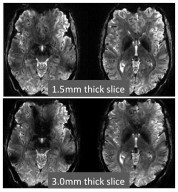
Comparison of a 1.5mm thick slice and a 3.0mm slice acquired at 7T using a single shot gradient echo EPI sequence (TE=25ms) with 1mm in-plane resolution. The through-plane dephasing produced by the susceptibility gradients is significantly reduced with thinner slices. Data courtesy of Christina Triantafyllou of MIT and MGH.

2.1.2 Partial volume reduction

High spatial resolution can help isolate the signal from gray matter. This reduces partial volume dilution with WM and CSF and also helps prevent partial volume contamination from unactivated cortex on the other side of a gyral fold. Reducing the partial volume effects has the simple benefit of increasing the BOLD Contrast to Noise Ratio (CNR) by avoiding dilution with unresponsive tissue (WM and CSF).

It is not possible to fit a 3mm voxel into most of the cortical ribbon without some dilution. Bringing the standard fMRI acquisition to 2mm isotropic at least allows for some voxels that are uncontaminated with WM or CSF. Figure 2 shows a partial volume analysis for ~5000 1mm isotropic voxels contacting 10 different cortical depth contours in area visual area V1. Note that even at high spatial resolution significant partial volume effects are present.

Fig. 2.

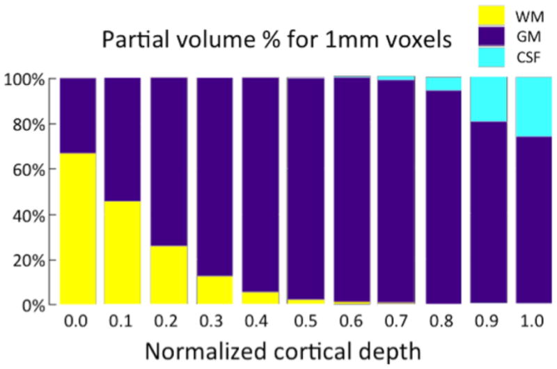
Partial volume analysis for ~5000 1mm isotropic voxels contacting 10 different cortical depth contours in area visual area V1. Note that even at 1mm spatial resolution, significant partial volume effects are present. Figure courtesy of Jon Polimeni of MGH.

2.1.3 Reducing CSF contamination

Beyond simple dilution with non-responsive material, the presence of CSF in the voxel is a source of noise contamination. This is due to the fact that CSF contains the highest level of nuisance fluctuations in in the fMRI time-series of the three basic compartments in the brain. (Bianciardi et al. 2009) Figure 3 shows a map of the standard deviation in the time series (physiological noise map) for a 1.5mm × 1.5mm × 3mm 3T acquisition. At high spatial resolution, these noise maps are essentially CSF maps, and increased ability to isolate the analyzed voxels to within the cortex can decrease the noise (by avoiding high variance CSF in the voxel.)

Fig. 3.

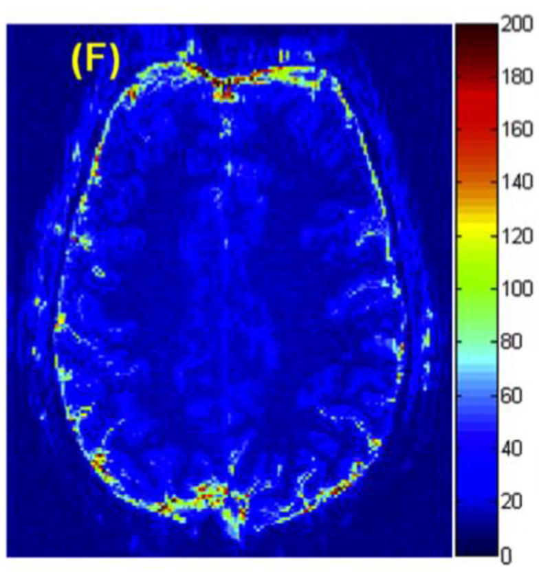
A map of the standard deviation in the time series (thermal + physiological noise map) for a 1.5mm × 1.5mm × 3mm 3T acquisition. At high spatial resolution, The dominance of the CSF fluctuations can be appreciated. This suggests that sufficient spatial resolution to limit the analyzed voxels to within the cortex can increase the BOLD CNR through increasing the signal change (by reducing dilution with unactivated tissue) and decreasing the noise (by avoiding high variance CSF in the voxel.) Figure courtesy of Christina Triantafyllou of MIT and MGH.

2.1.4 Reduction of physiological noise

The time-series SNR maps (each voxel’s signal mean divided by its time-series SD) of low resolution fMRI time-series are almost always physiological noise dominated. (Kruger et al. 2001; Triantafyllou et al. 2009; Hutton et al. 2011; Triantafyllou et al. 2011) These nuisance fluctuations behave differently from thermal noise as the voxel volume is changed at acquisition.(Triantafyllou et al. 2005) At a fixed readout bandwidth, thermal noise is an independent additive baseline to the BOLD signal changes that remains constant in amplitude as the voxel volume is changed. However, the physiological noise amplitude scales with the signal strength and thus with the voxel volume. (Kruger and Glover 2001) Thus, we find ourselves in the interesting situation where decreasing the signal (e.g. by reducing the voxel volume), also lowers the noise in the time-series. Since both signal and time-series noise decrease with voxel size, the result is a constant CNR as the resolution is increased. Thus, for physiological noise dominated acquisitions CNR will only increase if the improved resolution results in a reduction of partial volume dilution with un-activated tissue.

An alternative “glass-half-full” view suggests that strategies which reduce signal levels or add image noise (such as SENSE or GRAPPA) will not reduce BOLD CNR as much as might be imagined from looking at the degradation in SNR in the images themselves. In these cases a relatively large reduction in image SNR can be present with only a modest decrease in tSNR. For example, the time-series SNR is not as devastated by decreasing the voxel volume as the image SNR.(Triantafyllou et al. 2005) Additionally, for physiological noise dominated acquisitions, the g-factor noise introduced by parallel imaging effects the image SNR but is not as harmful to temporal SNR as the g-factor map suggests. (de Zwart et al. 2002) It can become beneficial to acquire physiological noise dominated data at a higher spatial resolution than needed for true resolution purposes and then spatially smooth the images. (Lowe et al. 1997; Triantafyllou et al. 2006) This is not a beneficial strategy for thermal noise dominated Fourier images.

2.1.5 Reducing pial vein contamination

Polimeni et al was able to show that the biological Point Spread Function (PSF) of an activation in V1 could be improved by limiting the analysis to voxels which did not directly contact the pial surface, using 1mm isotropic resolution at 7T with sufficient mitigation of susceptibility distortions to allow a precision alignment to the cortical surface. (Polimeni et al. 2010) Thus, “vein avoidance” by analyzing only the mid to deeper layers of the cortex offers a method to improve the biological PSF of BOLD activation and better localize activation. This comes at some cost in sensitivity since the pial signal (and its veins) gives the strongest BOLD effect in gradient echo acquisitions. (Zhao et al. 2004; Zhao et al. 2006) It is also important to note that the extra-vascular BOLD signal extends beyond the veins themselves. This, together with the presence of numerous diving venules, makes it impossible to fully avoid the delocalized effect of the veins by simply ignoring the pial layer. The Spin Echo acquisition offers an alternative method for large vein avoidance. (Boxerman et al. 1995; Lee et al. 1999) This will not be reviewed here since it is the topic of a separate paper in this issue. (Norris 2011)

2.2 Whole brain coverage

The brain requires about 120mm of coverage in the Superior to Inferior directions (~80 1.5mm axial slices) including the cerebellum. For coronal acquisition, 175mm of coverage is needed (~117 1.5mm slices), and for sagittal slices about 140mm of coverage is needed. A typical state-of-the-art scanner using modest acceleration can acquire 18x 3mm resolution slices per second of TR time. At higher resolution this drops (15 at 2mm, 13 at 1.5mm and 11 at 1mm). Thus, the TR times are currently longer than that desired for temporal resolution even for 3mm in-plane resolution (see 2.3 for estimates of desired TR times). Unfortunately, the need to image at a TE that optimizes BOLD contrast means that in-plane acceleration with parallel imaging only marginally improves this problem. Future acquisitions will have to accelerate in the slice direction to significantly impact this problem (prospects for this are discussed below).

2.3 Temporal Resolution

A few years ago, the goal of sub-second whole-brain acquisitions seemed unachievable, especially if spatial resolution is also improved. Recent advances in parallel imaging which focus on obtaining multiple slices simultaneous in time (discussed below) are poised to substantially narrow this gap.

The whole brain acquisition of the future should have adequate temporal resolutions to Nyquist sample the highest frequencies present in the Hemodynamic Response Function (HRF). For typically hemodynamic impulse responses, characterized by a FMHM of 4s(de Zwart et al. 2005), this would require a TR of about 2s. To characterize onset-times, which range from 0.59s to 1.27s in the rat (Silva et al. 2002) an even faster acquisition is needed. Sufficient temporal resolution to Nyquist sample nuisance fluctuations which follow the respiratory and cardiac cycle require a TR of about 0.5s or higher. Figure 4 shows the frequency spectrum of an fMRI time-series which was acquired with a highly accelerated (R=4×4) 64×64×56 matrix single-shot Echo Volume Imaging (EVI) sequence with a TR of 120ms. Note also that the primary nuisance fluctuations (physiological noise) is in a spectral region overlapping with that expected from the stimulus, so we can not expect huge gains from removing only the fluctuations at the respiratory and cardiac frequencies. However, the shorter TR insures that fluctuations from these cycles do not alias into the band of (low) frequencies containing the BOLD response and important resting state fluctuations.

Fig. 4.

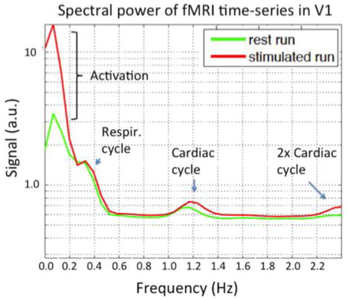
Spectral power in the visual cortex of a high temporal resolution dataset (TR=120ms) acquired with single shot EVI. The 3T data used a 32ch coil to achieve a R= 4×4 fold accelerated EVI trajectory with 6/8 partial Fourier acquisition of a 64×64×56 matrix over a 220mm FOV. Thus, of the 64×56=3584 lines that would need to be acquired, only 168 lines were acquired. The high temporal resolution allows the signal modulations at the frequencies of the respiratory, cardiac and second harmonic of the cardiac cycle to be seen. By Nyquist sampling at sufficient speed, these nuisance fluctuations can be removed by simple low-pass filtering. Figure courtesy of Thomas Witzel, MGH.

2.4 Image Distortion

Single shot echoplanar imaging suffers from local image distortions in the vicinity of susceptibility gradients. The magnitude of these distortions is proportional to the rate of transversal of kspace. Since EPI traverses the phase encode direction, k_y, more slowly than the readout direction the distortion is considerably larger in the y direction. Several readout parameters effect the displacement of the imaging voxel resulting from an off-resonance shift ΔB₀ from a susceptibility gradient. The most directly relevant parameter is the echospacing (esp). Esp is defined as half the period of the readout waveform and is the time between samples of k_y = 0 points in a fully sampled EPI trajectory. Typical echospacings used on a Siemens Tim Trio whole-body scanner are 0.47ms, 0.69ms 0.76ms, and 1.04ms for 3mm, 2mm, 1.5mm and 1mm isotropic resolutions respectively. When accelerated by a factor of R_y using parallel imaging, the parameter relevant to kspace velocity and thus distortion is the effective echospacing; esp_eff = esp/R_y. Related, but less useful parameters for characterizing distortion include the total EPI readout length (T_read) and the number of phase encode lines; N_y. These do not necessarily reflect distortion since it is possible to reduce the readout time without reducing the rate of traversal of kspace, for example by using partial Fourier acquisition.

The bandwidth across the final reconstructed image FOV_y, (after SENSE or GRAPPA) is 1/esp_eff. Thus, a frequency shift of Δv = 1/esp_eff would shift a voxel by an entire FOV. Perhaps the most relevant metric is the distortion in millimeters for a unit ΔB₀ shift. This metric is:

$$\left(\mathit{distortion}[mm]/\mathrm{\Delta }{B}_0\right)=\frac{\gamma }{2\pi }{\mathit{esp}}_{\mathit{eff}}•{\mathit{FOV}}_y[mm]=\frac{\gamma }{2\pi }\frac{\mathit{esp}•{\mathit{FOV}}_y[mm]}{R_y}.$$ Eq. 1

By this distortion metric, the acquisition of the future must decrease distortions through either reducing esp (faster, stronger gradients), increasing R_y (larger parallel imaging acceleration factors), or reducing the phase encode FOV (zoomed imaging).

2.5 Motion Mitigation

Motion of the head during the fMRI acquisition is an important issue, especially for uncooperative subject populations such as young children and certain patient populations such as those with Alzheimers disease or Autism. Ideally, the scanner should independently track the rigid body motion of the head in real-time and continuously update the acquisition coordinate system appropriately. Such a scheme goes beyond eliminating the need for retrospective motion correction by removing significant variance in the fMRI time-series (from movement induced spin-history effects.) Prospective motion correction has been implemented using the images in the time-series themselves to detect motion (Thesen et al. 2000), but the resulting feedback time of several seconds is too slow to correct the effects of many motions. What is needed is an independent system to measure the 6 motion parameters with high sensitivity and temporal resolution. There are many candidate sensors available using optical video tracking devices or magnetic field probes which can measure position using the scanners gradient fields. A common issue to all external tracking devices is finding a subject-friendly way to attach the fiducial to the skull. The most workable method is attachment to the upper teeth. Attachment to the skin is problematic in that movements of the facial muscles might cause the system to adjust the image coordinate system when no brain motion is present. While the fast external system is perhaps ideal, many simpler developments in engineering the RF array coil to better immobilize the head would also improve many acquisitions.

3. Prospective technologies for improved fMRI acquisition

3.1 Higher field strength

The benefit of acquiring BOLD functional imaging data at higher field strength is often summarized as improved sensitivity to subtle activation and improved spatial specificity to the site of neuronal activation. The physical and biological mechanisms behind this are complex, but the empirical data support these broad claims and has driven the steady increase in the field strength of scanners used for these experiments as well as a continuous investigation of techniques to maximize sensitivity and spatial specificity.

Contrast to Noise Ratio (CNR) is the signal intensity difference (ΔS) between the activated and non-activated state divided by the noise standard deviation of the time-series (σ_total). As such, it is the most important metric of fMRI detection since it provides a measure of the smallest activations that can be detected and determines the statistical importance of a stronger or weaker activation in a population. The improvement in BOLD Contrast to Noise Ratio (CNR) at higher field strength is best understood by examining the factors comprising CNR. Starting with its definition: CNR = ΔS/σ_total, CNR can be rewritten in a useful way by multiplying by S/S and using the definition of the time-series Signal to Noise Ratio (tSNR = S/σ_total). Then: CNR = tSNR (ΔS/S). This expression alone is informative in that it clearly shows the importance of tSNR in the fMRI experiment (as well as that of the % signal change, ΔS/S).

It is helpful to further explore the factors behind ΔS/S. S can be written from the resting state signal present at the echo-time TE; S = S₀ exp(−TE/T_2rest^*). Then ΔS is the difference between the signal in the activated and baseline state;

$$\mathrm{\Delta }\text{S}={\text{S}}_{0}exp(-\text{TE}/{{\text{T}}_{2\text{rest}}}^{\ast })-{\text{S}}_{0}exp(-\text{TE}/{{\text{T}}_{2\text{active}}}^{\ast })$$

Dividing by S gives; ΔS/S = 1 − exp(−TE(1/T_2rest^* − 1/T_2active^*)). We can express the difference in relaxation times in terms of a difference in relaxation rates, ΔR₂*, where R = 1/T₂^*. Then:

$$\mathrm{\Delta }\text{S}/\text{S}=1-exp(-\text{TE}\mathrm{\Delta }{{\text{R}}_2}^{\ast })\approx -\text{TE}\mathrm{\Delta }{{\text{R}}_2}^{\ast }.$$

Here we have assumed small activation changes (ΔR₂*≪ 1), replacing the exponential exp(−TE ΔR₂*) in ΔS/S by the first two terms of its power series expansion providing Substituting this back into CNR = tSNR (ΔS/S) gives:

$$\text{CNR}=-\text{tSNR}\text{TE}\mathrm{\Delta }{{\text{R}}_2}^{\ast }$$ Eq. 2

In this view, only three factors contribute to the BOLD acquisition CNR; tSNR, TE and ΔR₂*. The tSNR is not much changed when the field strength is pressed beyond 3T unless relatively high resolution acquisitions are used where thermal noise dominates over physiological noise sources. (Triantafyllou et al. 2005) In this case, tSNR increases linearly with B₀. Typically TE is set to the local T₂* value or a bit lower as a good approximation of the TE which optimizes BOLD CNR. Setting TE=1/R₂^* gives CNR = −tSNR (ΔR₂*/R₂*). That leaves ΔR₂*/R₂* as the only parameter by which BOLD CNR can benefit in conventional physiological noise dominated acquisitions at higher field. Note ΔR₂*/R₂* derives from the biological response of the tissue and is field dependent, but not dependent on other acquisition sequence choices (except, of course that TE is set to T₂^* for the tissue). Also note that since ΔS/S is equal to ΔR₂*/R₂*, percent signal change too is mainly dependent on biological factors interacting with the static magnetic field.

Equation 2 shows that most acquisition parameters such as coil choice, parallel imaging acceleration, and voxel size affect BOLD CNR through tSNR. Fortunately this is very easy to measure from the experimental data and should be carefully monitored in every run. Note also that the percent signal change only depends on the biological response when TE is properly set. A classic beginner’s error is to use ΔS/S in the comparison of head coils or other acquisition parameters to which it is not expected to be sensitive.

Several studies have confirmed what is expected from dephasing around magnetized cylinders, namely that ΔR₂* and (R₂*/ΔR₂*) increase with field strength. (Turner et al. 1993; Bandettini et al. 1994; Gati et al. 1997) (Yacoub et al. 2001; Cohen et al. 2009) For example, Gati et al. report ΔR₂*/R₂* = 0.014, 0.022, and 0.35 for the tissue component at 0.5T, 1.5T and 4T and Yacoub and colleagues measurement of gray matter ΔR₂* and T₂^* give ΔR₂*/R₂* = 0.034, 0.048 at 4T and 7T respectively when TE=T₂^*.

While 7T has established itself for high resolution functional imaging based on the “double win” of increased tSNR and ΔR₂*/R₂*, it has yet to establish itself for applications which do not fully demand high resolution acquisitions (e.g. many cognitive neuroscience experiments) where it offers only the “single win” of increased ΔR₂*/R₂*. Nuisances of moving to higher field strength include increased cost, increased susceptibility gradients (and therefore image distortion in EPI), and biological effects on the subject like dizziness and vertigo.

3.2 Improved gradients

Much of the image quality improvements gained in single shot imaging over the last 20 years can be attributed to the four-fold increase in gradient strength that has occurred over this period. Both slew-rate and gradient strength are important to minimize the esp of the EPI readout and thus the image distortion of Eq. 1. Relative to the current state-of-the-art whole body gradient (G_max = 40mT/m and slew rate = 200 T/m/s), standard resolution EPI (3mm) would benefit mainly from increased slew rate. High resolution (1mm) benefits from both increased G_max and slew rate. Peripheral nerve stimulation is one of the primary issues blocking further gradient improvements from further reducing the EPI echospacing. (Schenck 2000; Schenck 2005) Simply driving the standard gradient set with more current and voltage would produce shorter readouts but cause painful peripheral nerve stimulation. For example, the Human Connectome Project in our laboratory uses a G_max = 300mT/m human gradient set capable of slewing at 200T/m/s. While extremely helpful for diffusion encoding, such high gradient strengths used at full slew rate for the EPI readout is not practical due to stimulation concerns. A move toward smaller, head-sized linear regions helps somewhat in reducing peripheral nerve stimulation in whole body gradients. Head gradients can slew even faster without nerve stimulation since their fields do not extend into the shoulders. They have achieved impressive results (reducing esp by nearly a factor of 2 in 3mm imaging). Unfortunately, head gradients have provide limited space for RF arrays and stimulation equipment.

New ideas for gradient encoding are also emerging. These involve moving beyond the Fourier encoding basis provided by spatially linear encoding fields (gradients). While this direction was examined in the past for local gradients (Patz et al. 1999), they are currently being re-examined as an array of multiple independently driven coils for their potential to avoid the limits imposed by stimulation. (Hennig et al. 2008) Additionally, encoding field arrays are being examined to potentially find a non-Fourier basis set which maximally complements the spatial patterns in the RF array (used to encode in parallel imaging.) (Stockmann et al. 2010) While uncovering some interesting imaging physics, the jury is still out about the overall utility of this direction.

3.3 Highly parallel imaging

Advances in RF technology, have proved a valuable and cost-effective way to improve sensitivity and encoding capabilities of fMRI. In its beginning years, whole brain fMRI was performed with a single-channel volume birdcage coil. The introduction of the MR phased array in 1990 showed the sensitivity benefit of receiving the MR signal with multiple smaller coils. (Roemer et al. 1990) The second breakthrough was methods to replace gradient encoding with the spatial information present in the detected signal pattern; the SENSE (Pruessmann et al. 1999) and SMASH (Sodickson et al. 1997) (and ultimately GRAPPA (Griswold et al. 2002)) methods. Acquiring only every other or every third kspace line in the EPI readout shortens the readout, reducing T₂^* blurring and more importantly increasing the rate of traversal of kspace. This kspace velocity increase has made parallel acquisition our primary tool for reducing susceptibility induced distortions (see Eq. 1).

Increased reliance on the array as a primary device for image encoding will likely lead to considerably higher numbers of detectors than would be contemplated from sensitivity arguments alone. In this scenario, the role of the MR detector array begins to more resemble the electroencephalography (EEG) or magnetoencephalography (MEG) detector where all of the spatial information is derived from the detector geometry. So far, brain arrays have been tested with 32, 64 and 96 channels. (Wiggins et al. 2006; Wiggins et al. 2009; Keil et al. 2012) These results (and simulations(Wiesinger et al. 2004; Wiesinger et al. 2005)) show that as channels are added, the SNR in unaccelerated imaging in the brain center approaches an asymptotic limit. The increased SNR above 32ch is primarily peripheral. For accelerated imaging, however, the highly-aliased brain center receives the brunt of the g-factor noise amplification, and this noise amplification is lowered in larger arrays. In this way, the highly parallel array can significantly benefit sensitivity in the image center. Simulation and practical issues suggest that this benefit will also eventually reach an asymptote.(Wiesinger et al. 2004; Wiesinger et al. 2005) Figure 5 shows these effects in the comparison of a 32ch and a 64ch brain array constructed on an identical former. In the un-accelerated scan, the benefit of the 64 channel is a factor of 1.05, 1.1 and 1.7 fold SNR improvement for the brain center, deep cortex, and peripheral cortex respectively. However, for the R=4 accelerated scan, the SNR improvement of the 64ch array was 1.26x in the brain center and 1.8x in the periphery.

Fig. 5.

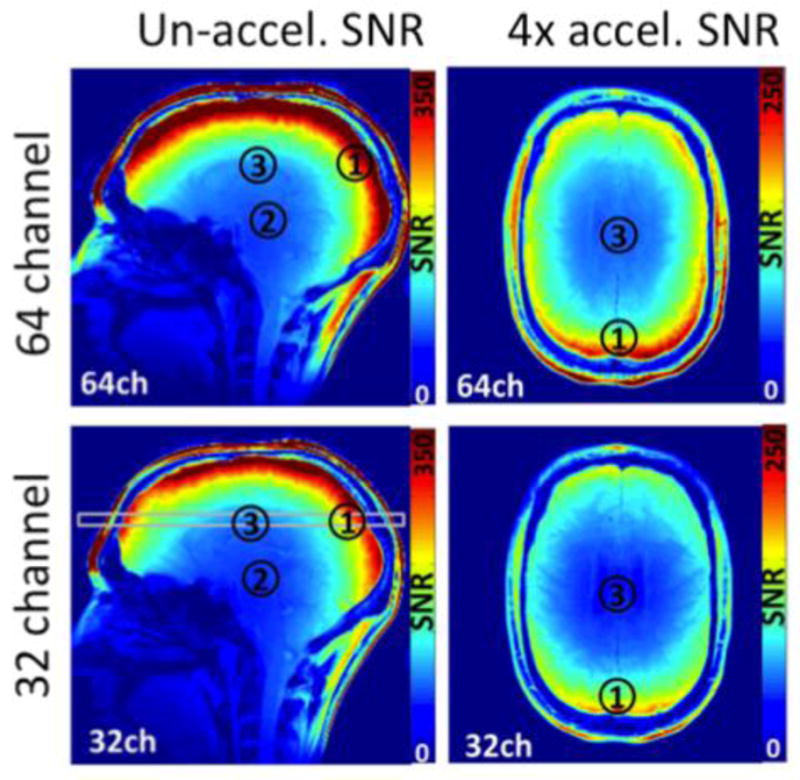
SNR comparison between a 32ch and 64ch brain array built on matched close-fitting shells. The gain from the 2 fold increase in channels for unacclerated imaging is only in the periphery for un-accelerated imaging. For accelerated imaging, the center of the brain also benefits. In the un-accelerated scan, the benefit of the 64 channel is a factor of 1.05, 1.1 and 1.7 fold SNR improvement for the brain center, more superior central, and periphery. For the R=4 accelerated scan, the SNR improvement of the 64ch array was 1.26x in the brain center and 1.8x in the periphery. Figure courtesy of Boris Keil, MGH.

Highly parallel array coils and accelerated imaging cause some problems as well as the benefits discussed above. The most problematic issue is the increased sensitivity to motion. Part of the problem arises from the use of reference data or coil sensitivity maps taken at the beginning of the scan. Movement then leads to changing levels of residual aliasing in the time-series. A second issue derives from the spatially varying signal levels present in an array coil image. Even after perfect rigid-body alignment (motion correction), the signal time-course in a given brain structure will be modulated by the motion of that structure through the steep sensitivity gradient. Motion correction (prospective or retrospective) brings brain structures into alignment across the time-series but does not alter their intensity changes incurred from moving through the coil profiles of the fixed-position coils. This effect can be partially removed by regression of the residuals of the motion parameters; a step that has been shown to be very successful in removing nuisance variance in ultra-high field array coil data. (Hutton et al. 2011) An improved strategy might be to model and remove the expected nuisance intensity changes using the motion parameters and the coil sensitivity map.

3.4 Shimming

Improving shimming for fMRI is another promising area for improving the fMRI acquisition. Driven partially by the need to reduce EPI distortion, second order shimming has become standard in state-of-the-art clinical scanners. The benefits of higher order spherical harmonic coils has been examined (Kim et al. 2002) as well as the benefit of dynamically adjusting the linear (Morrell et al. 1997) and higher order terms.(de Graaf et al. 2003) (Koch et al. 2006; Juchem et al. 2010; Sengupta et al. 2011) (Hillenbrand et al. 2005) Passive shim materials(Juchem et al. 2006; Yang et al. 2011) (Koch et al. 2006) (Hillenbrand et al. 2005) or multicoil shims(Juchem et al. 2011) provide alternative approaches to correcting spatial patterns above 3^rd order. These approaches are achieving impressive results in prototype form, and hopefully will make the transition to clinical scanners.

3.5 Sequences; Echo-volume and Simultaneous MultiSlice (SMS) acquisitions

A key insight into improving the encoding efficiency in fMRI is gained by noting the inefficiency of sampling with a TR significantly longer than T₁. In this case the magnetization of the sampled slice sits un-used and fully relaxed waiting for the other slices to be sampled. A better strategy is to excite and encode multiple slices simultaneously and then readout these slices simultaneously. This is achieved in either a true 3D approach such as Echo Volume Imaging (EVI) or a pseudo-volume strategy where multiple slices are excited and read-out simultaneously and unaliased with parallel imaging. The latter, was originally described by Larkman et al. a decade ago (Larkman et al. 2001) as the separation of signals from “slices simultaneously excited.” Recent implementations(Feinberg et al. 2010; Moeller et al. 2010) and an EPI specific improvement(Setsompop et al. 2011) have been referred to as Multi-Band (MB) imaging and Simultaneous Multi-Slice (SMS) respectively.

Both EVI and SMS methods rely heavily on parallel imaging to encode the spatial data. EVI incurs the standard SNR penalty of g √R, while SMS incurs only the g-factor penalty. This is because the SMS method does not leave out data samples. (Larkman et al. 2001) Instead a modulated RF pulse excites 2 or more slices simultaneously and the aliased slices are disentangled using parallel imaging methods such as slice-SENSE(Larkman et al. 2001) or slice-GRAPPA(Blaimer et al. 2006) (Setsompop et al. 2011). Thus the image SNR is reduced by the g factor, but not by a factor of √R.

Figures 6 and 7 shows an acquisition acquired with state-of-the-art EVI and SMS. While the EVI is impressive (acquiring the whole brain in a TR of 120ms), the SMS method with a R_slice factor of 6 retains very high image quality and is capable of fulfilling most of our temporal resolutions needs (TR<1s for 2mm EPI).

Fig. 6.

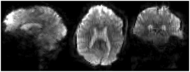
Single shot, whole-brain 3T Echo Volume Imaging (EVI) brain volume. This single shot volume image, shown in axial, coronal and sagittal planes was acquired in single shot allowing whole-brain acquisitions with a temporal resolution of 120ms. The matrix was 64×64×56 wutg a 24cm FOV, resulting in 3.4mm nominal spatial resolution. The duration of the GRAPPA accelerated, 6/8 partial Fourier trajectory was 77.3ms resulting in some spatial blurring. The effective echospacing in the slowest phase encode direction was 1.38ms resulting in relatively high (compared to 2D EPI) distortions. Image courtesy of Thomas Witzel, MGH.

Fig. 7.

Simultaneous-MultiSlice (SMS) EPI acquisition, 1mm isotropic resolution taken at 7T using 3 slices simultaneously excited and R=2 in-plane GRAPPA, 120 slices acquired with a TR = 2.88s. The acquisition used in-plane CAIPIRINHIA style shifts between the slices of FOV/3. Without the R_slice = 3 slice acceleration, the minimum TR would have been 8.64s and unable to capture the relevant bandwidth for resting-state studies. Image courtesy of Kawin Setsompop, MGH.

3.6 Parallel Transmit

Parallel transmission (pTx) uses multiple excitation coils driven by independent RF pulse waveforms to allow individual control over the spatially separate transmit fields with temporally distinct RF pulse waveforms. This creates spatial degrees of freedom that allow the spatial information in the array to be exploited in the excitation process. For fMRI, the most pressing applications are to achieve a uniform excitation flip-angle pattern in the head at 7T and to allow the excitation of user-defined shaped excitation for zoomed imaging (imaging a specific region with a reduced FOV.) The flip-angle variations across the head are not severe for 90° excitations in 7T gradient echo fMRI. For example, deviations of ±20° from the target flip-angle result in only a 6% change in intensity. None-the-less, where the B₁⁺ field cancellation is severe, such as the inferior temporal lobes, the loss in SNR can be as much as a factor of 2. Parallel transmission at 7T using 8 transmit coils and a 3D volume kspace pattern for excitation can successfully mitigate this problem. (Setsompop et al. 2008) More intensive kspace trajectories have been used to carve out anatomy specific regions(Katscher et al. 2006), a scheme which allows the FOV of the EPI to be reduced (“zoomed” EPI (Pfeuffer et al. 2002)) and therefore achieve reduced susceptibility distortions. Finally, Stenger’s group has introduced a novel pTx method to reduce susceptibility dropouts from through-plane dephasing in specific areas, such as the orbital-frontal cortex. (Deng et al. 2009) This scheme time-shifts the slice selective excitations for the coils exciting the problem area. This is equivalent to applying a z-shim rephrasing lobe to this region.

It seems likely that parallel transmit will become widely implemented despite its technical difficulties (especially in SAR monitoring) due to its clinical utility in body imaging at 3T. But its impact on fMRI will be largely focused on acquisitions at 7T and above.

4. Conclusions

The last 2 decades of improvements in fMRI acquisition have been impressive. “Acquisition engineering” has left the field with considerable gains in sensitivity from advanced RF array designs and higher field strengths to considerably cleaner, faster, less distorted single-shot imaging with improved gradients and parallel imaging acceleration. None-the-less, future needs in image quality and spatial and temporal resolution are still considerable. Luckily, a long list of technologies are at different stages of development and offer considerable promise for future improvements. They attack the problem at the acquisition hardware level through the “coils” of MRI; gradient, shim, transmit and receive. They also address our problems through acquisition and reconstruction software (e.g. EVI and SMS), and time-series postprocessing such as variance removal of motion induced and biological effects (vein and CSF avoidance). While progress will appear slow, and developments initially only benefits a single laboratory, successful acquisition developments will ultimately impact all practitioners and their impact on the field temporally integrates over time.

Highlights.

The goal of this paper is to get an advanced look at the capabilities of the fMRI acquisition methods of the near future. The unmet needs of the fMRI acquisition are described along with a number of acquisition technologies currently under development.

References

- Bandettini PA, Wong EC, Jesmanowicz A, Prost R, Cox RW, Hinks RS, Hyde JS. MRI of human brain activation at 0.5 T, 1.5 T and 3.0 T: comparisons of ΔR2*, and functional contrast to noise ratio. Proceedings of the second annual meeting of the Society of Magentic Resonance in Medicine; San Francisco. 1994. [Google Scholar]
- Bianciardi M, Fukunaga M, van Gelderen P, Horovitz SG, de Zwart JA, Shmueli K, Duyn JH. Sources of functional magnetic resonance imaging signal fluctuations in the human brain at rest: a 7 T study. Magnetic resonance imaging. 2009;27(8):1019–1029. doi: 10.1016/j.mri.2009.02.004. [DOI] [PMC free article] [PubMed] [Google Scholar]
- Blaimer M, Breuer FA, Seiberlich N, Mueller MF, Heidemann RM, Jellus V, Wiggins G, Wald LL, Griswold MA, Jakob PM. Accelerated volumetric MRI with a SENSE/GRAPPA combination. J Magn Reson Imaging. 2006;24(2):444–450. doi: 10.1002/jmri.20632. [DOI] [PubMed] [Google Scholar]
- Boxerman JL, Hamberg LM, Rosen BR, Weisskoff RM. MR contrast due to intravascular magnetic susceptibility perturbations. Magnetic resonance in medicine: official journal of the Society of Magnetic Resonance in Medicine/Society of Magnetic Resonance in Medicine. 1995;34(4):555–566. doi: 10.1002/mrm.1910340412. [DOI] [PubMed] [Google Scholar]
- Buxton RB. Introduction to Functional Magnetic Resonance Imaging, Principles and Techniques. 2. Cambridge: Cambridge University Press; 2009. pp. 262–265. [Google Scholar]
- Cohen ER, O’Neill JM, Joffres M, Upshur RE, Mills E. Reporting of informed consent, standard of care and post-trial obligations in global randomized intervention trials: a systematic survey of registered trials. Developing world bioethics. 2009;9(2):74–80. doi: 10.1111/j.1471-8847.2008.00233.x. [DOI] [PubMed] [Google Scholar]
- de Graaf RA, Brown PB, McIntyre S, Rothman DL, Nixon TW. Dynamic shim updating (DSU) for multislice signal acquisition. Magnetic resonance in medicine: official journal of the Society of Magnetic Resonance in Medicine/Society of Magnetic Resonance in Medicine. 2003;49(3):409–416. doi: 10.1002/mrm.10404. [DOI] [PubMed] [Google Scholar]
- de Zwart JA, Silva AC, van Gelderen P, Kellman P, Fukunaga M, Chu R, Koretsky AP, Frank JA, Duyn JH. Temporal dynamics of the BOLD fMRI impulse response. NeuroImage. 2005;24(3):667–677. doi: 10.1016/j.neuroimage.2004.09.013. [DOI] [PubMed] [Google Scholar]
- de Zwart JA, van Gelderen P, Kellman P, Duyn JH. Application of sensitivity-encoded echo-planar imaging for blood oxygen level-dependent functional brain imaging. Magnetic resonance in medicine: official journal of the Society of Magnetic Resonance in Medicine/Society of Magnetic Resonance in Medicine. 2002;48(6):1011–1020. doi: 10.1002/mrm.10303. [DOI] [PubMed] [Google Scholar]
- Deichmann R, Josephs O, Hutton C, Corfield DR, Turner R. Compensation of susceptibility-induced BOLD sensitivity losses in echo-planar fMRI imaging. NeuroImage. 2002;15(1):120–135. doi: 10.1006/nimg.2001.0985. [DOI] [PubMed] [Google Scholar]
- Deng W, Yang C, Alagappan V, Wald LL, Boada FE, Stenger VA. Simultaneous z-shim method for reducing susceptibility artifacts with multiple transmitters. Magnetic resonance in medicine: official journal of the Society of Magnetic Resonance in Medicine/Society of Magnetic Resonance in Medicine. 2009;61(2):255–259. doi: 10.1002/mrm.21870. [DOI] [PMC free article] [PubMed] [Google Scholar]
- Feinberg DA, Moeller S, Smith SM, Auerbach E, Ramanna S, Glasser MF, Miller KL, Ugurbil K, Yacoub E. Multiplexed echo planar imaging for sub-second whole brain FMRI and fast diffusion imaging. PLoS ONE. 2010;5(12):e15710. doi: 10.1371/journal.pone.0015710. [DOI] [PMC free article] [PubMed] [Google Scholar]
- Gati JS, Menon RS, Ugurbil K, Rutt BK. Experimental determination of the BOLD field strength dependence in vessels and tissue. Magnetic resonance in medicine: official journal of the Society of Magnetic Resonance in Medicine/Society of Magnetic Resonance in Medicine. 1997;38(2):296–302. doi: 10.1002/mrm.1910380220. [DOI] [PubMed] [Google Scholar]
- Griswold MA, Jakob PM, Heidemann RM, Nittka M, Jellus V, Wang J, Kiefer B, Haase A. Generalized autocalibrating partially parallel acquisitions (GRAPPA) Magnetic resonance in medicine: official journal of the Society of Magnetic Resonance in Medicine/Society of Magnetic Resonance in Medicine. 2002;47(6):1202–1210. doi: 10.1002/mrm.10171. [DOI] [PubMed] [Google Scholar]
- Hahn ELLL. Wald [Google Scholar]
- Hahn EL. NMR and MRI in Retrospect. Philosophical Transactions of the Royal Society of London: Physical Sciences and Engineering. 1990;333(1632):403–411. [Google Scholar]
- Hennig J, Welz AM, Schultz G, Korvink J, Liu Z, Speck O, Zaitsev M. Parallel imaging in non-bijective, curvilinear magnetic eld gradients: a concept stud. Magn ResonMater Phys. 2008;2008(21):5–14. doi: 10.1007/s10334-008-0105-7. [DOI] [PMC free article] [PubMed] [Google Scholar]
- Hillenbrand DF, Lo KM, Punchard WFB, Resse TG, Starewicz P. High-Order MR Shimming: a Simulation Study of the Effectiveness of Competing Methods, Using an Established Susceptibility Model of the Human Head. Applied Magnetic Resonance. 2005;29:39–64. [Google Scholar]
- Hutton C, Josephs O, Stadler J, Featherstone E, Reid A, Speck O, Bernarding J, Weiskopf N. The impact of physiological noise correction on fMRI at 7T. NeuroImage. 2011;57(1):101–112. doi: 10.1016/j.neuroimage.2011.04.018. [DOI] [PMC free article] [PubMed] [Google Scholar]
- Juchem C, Muller-Bierl B, Schick F, Logothetis NK, Pfeuffer J. Combined passive and active shimming for in vivo MR spectroscopy at high magnetic fields. Journal of magnetic resonance. 2006;183(2):278–289. doi: 10.1016/j.jmr.2006.09.002. [DOI] [PubMed] [Google Scholar]
- Juchem C, Nixon TW, Diduch P, Rothman DL, Starewicz P, de Graaf RA. Dynamic Shimming of the Human Brain at 7 Tesla. Concepts in magnetic resonance Part B, Magnetic resonance engineering. 2010;37B(3):116–128. doi: 10.1002/cmr.b.20169. [DOI] [PMC free article] [PubMed] [Google Scholar]
- Juchem C, Nixon TW, McIntyre S, Boer VO, Rothman DL, de Graaf RA. Dynamic multi-coil shimming of the human brain at 7T. Journal of magnetic resonance. 2011;212(2):280–288. doi: 10.1016/j.jmr.2011.07.005. [DOI] [PMC free article] [PubMed] [Google Scholar]
- Katscher U, Bornert P. Parallel RF transmission in MRI. NMR in biomedicine. 2006;19(3):393–400. doi: 10.1002/nbm.1049. [DOI] [PubMed] [Google Scholar]
- Keil B, Blau JN, Biber S, Hamm M, Wald LL. A 64-channel brain array coil for 3T imaging. Submitted: Proceedings of the ISMRM; Melbourne Australia. 2012. [Google Scholar]
- Kim DH, Adalsteinsson E, Glover GH, Spielman DM. Regularized higher-order in vivo shimming. Magnetic resonance in medicine: official journal of the Society of Magnetic Resonance in Medicine/Society of Magnetic Resonance in Medicine. 2002;48(4):715–722. doi: 10.1002/mrm.10267. [DOI] [PubMed] [Google Scholar]
- Koch KM, Brown PB, Rothman DL, de Graaf RA. Sample-specific diamagnetic and paramagnetic passive shimming. Journal of magnetic resonance. 2006;182(1):66–74. doi: 10.1016/j.jmr.2006.06.013. [DOI] [PubMed] [Google Scholar]
- Koch KM, McIntyre S, Nixon TW, Rothman DL, de Graaf RA. Dynamic shim updating on the human brain. Journal of magnetic resonance. 2006;180(2):286–296. doi: 10.1016/j.jmr.2006.03.007. [DOI] [PubMed] [Google Scholar]
- Kruger G, Glover GH. Physiological noise in oxygenation-sensitive magnetic resonance imaging. Magnetic resonance in medicine: official journal of the Society of Magnetic Resonance in Medicine/Society of Magnetic Resonance in Medicine. 2001;46(4):631–637. doi: 10.1002/mrm.1240. [DOI] [PubMed] [Google Scholar]
- Lai S, Glover GH. Three-dimensional spiral fMRI technique: a comparison with 2D spiral acquisition. Magnetic resonance in medicine: official journal of the Society of Magnetic Resonance in Medicine/Society of Magnetic Resonance in Medicine. 1998;39(1):68–78. doi: 10.1002/mrm.1910390112. [DOI] [PubMed] [Google Scholar]
- Larkman DJ, Hajnal JV, Herlihy AH, Coutts GA, Young IR, Ehnholm G. Use of multicoil arrays for separation of signal from multiple slices simultaneously excited. J Magn Reson Imaging. 2001;13(2):313–317. doi: 10.1002/1522-2586(200102)13:2<313::aid-jmri1045>3.0.co;2-w. [DOI] [PubMed] [Google Scholar]
- Lee SP, Silva AC, Ugurbil K, Kim SG. Diffusion-weighted spin-echo fMRI at 9.4 T: microvascular/tissue contribution to BOLD signal changes. Magnetic resonance in medicine: official journal of the Society of Magnetic Resonance in Medicine/Society of Magnetic Resonance in Medicine. 1999;42(5):919–928. doi: 10.1002/(sici)1522-2594(199911)42:5<919::aid-mrm12>3.0.co;2-8. [DOI] [PubMed] [Google Scholar]
- Lowe MJ, Sorenson JA. Spatially filtering functional magnetic resonance imaging data. Magnetic resonance in medicine: official journal of the Society of Magnetic Resonance in Medicine/Society of Magnetic Resonance in Medicine. 1997;37(5):723–729. doi: 10.1002/mrm.1910370514. [DOI] [PubMed] [Google Scholar]
- Moeller S, Yacoub E, Olman CA, Auerbach E, Strupp J, Harel N, Ugurbil K. Multiband multislice GE-EPI at 7 tesla, with 16-fold acceleration using partial parallel imaging with application to high spatial and temporal whole-brain fMRI. Magnetic resonance in medicine: official journal of the Society of Magnetic Resonance in Medicine/Society of Magnetic Resonance in Medicine. 2010;63(5):1144–1153. doi: 10.1002/mrm.22361. [DOI] [PMC free article] [PubMed] [Google Scholar]
- Morrell G, Spielman D. Dynamic shimming for multi-slice magnetic resonance imaging. Magnetic resonance in medicine: official journal of the Society of Magnetic Resonance in Medicine/Society of Magnetic Resonance in Medicine. 1997;38(3):477–483. doi: 10.1002/mrm.1910380316. [DOI] [PubMed] [Google Scholar]
- Norris DG. Spin-Echo fMRI: the poor relation? NeuroImage. 2011 doi: 10.1016/j.neuroimage.2012.01.003. current issue. [DOI] [PubMed] [Google Scholar]
- Patz S, Hrovat MI, Pulyer YM, Rybicki FY. Novel encoding technology for ultrafast MRI in a limited spatial region. Int J Imaging Syst Technol. 1999;10:216–224. [Google Scholar]
- Pfeuffer J, van de Moortele PF, Yacoub E, Shmuel A, Adriany G, Andersen P, Merkle H, Garwood M, Ugurbil K, Hu X. Zoomed functional imaging in the human brain at 7 Tesla with simultaneous high spatial and high temporal resolution. Neuroimage. 2002;17(1):272–286. doi: 10.1006/nimg.2002.1103. [DOI] [PubMed] [Google Scholar]
- Polimeni JR, Fischl B, Greve DN, Wald LL. Laminar analysis of 7T BOLD using an imposed spatial activation pattern in human V1. NeuroImage. 2010;52(4):1334–1346. doi: 10.1016/j.neuroimage.2010.05.005. [DOI] [PMC free article] [PubMed] [Google Scholar]
- Pruessmann KP, Weiger M, Scheidegger MB, Boesiger P. SENSE: sensitivity encoding for fast MRI. Magn Reson Med. 1999;42(5):952–962. [PubMed] [Google Scholar]
- Roemer PB, Edelstein WA, Hayes CE, Souza SP, Mueller OM. The NMR phased array. Magn Reson Med. 1990;16(2):192–225. doi: 10.1002/mrm.1910160203. [DOI] [PubMed] [Google Scholar]
- Schenck JF. Safety of strong, static magnetic fields. Journal of magnetic resonance imaging: JMRI. 2000;12(1):2–19. doi: 10.1002/1522-2586(200007)12:1<2::aid-jmri2>3.0.co;2-v. [DOI] [PubMed] [Google Scholar]
- Schenck JF. Physical interactions of static magnetic fields with living tissues. Progress in biophysics and molecular biology. 2005;87(2–3):185–204. doi: 10.1016/j.pbiomolbio.2004.08.009. [DOI] [PubMed] [Google Scholar]
- Sengupta S, Welch EB, Zhao Y, Foxall D, Starewicz P, Anderson AW, Gore JC, Avison MJ. Dynamic B0 shimming at 7 T. Magnetic resonance imaging. 2011;29(4):483–496. doi: 10.1016/j.mri.2011.01.002. [DOI] [PMC free article] [PubMed] [Google Scholar]
- Setsompop K, Alagappan V, Gagoski B, Witzel T, Polimeni J, Potthast A, Hebrank F, Fontius U, Schmitt F, Wald LL, Adalsteinsson E. Slice-selective RF pulses for in vivo B1+ inhomogeneity mitigation at 7 tesla using parallel RF excitation with a 16-element coil. Magnetic resonance in medicine: official journal of the Society of Magnetic Resonance in Medicine/Society of Magnetic Resonance in Medicine. 2008;60(6):1422–1432. doi: 10.1002/mrm.21739. [DOI] [PMC free article] [PubMed] [Google Scholar]
- Setsompop K, Gagoski BA, Polimeni JR, Witzel T, Wedeen VJ, Wald LL. Blipped-controlled aliasing in parallel imaging for simultaneous multislice echo planer imaging with reduced g-factor penalty. Magnetic resonance in medicine: official journal of the Society of Magnetic Resonance in Medicine/Society of Magnetic Resonance in Medicine. 2011 doi: 10.1002/mrm.23097. [DOI] [PMC free article] [PubMed] [Google Scholar]
- Silva AC, Koretsky AP. Laminar specificity of functional MRI onset times during somatosensory stimulation in rat. Proceedings of the National Academy of Sciences of the United States of America. 2002;99(23):15182–15187. doi: 10.1073/pnas.222561899. [DOI] [PMC free article] [PubMed] [Google Scholar]
- Sodickson DK, Manning WJ. Simultaneous acquisition of spatial harmonics (SMASH): fast imaging with radiofrequency coil arrays. Magnetic resonance in medicine: official journal of the Society of Magnetic Resonance in Medicine/Society of Magnetic Resonance in Medicine. 1997;38(4):591–603. doi: 10.1002/mrm.1910380414. [DOI] [PubMed] [Google Scholar]
- Stockmann JP, Ciris PA, Galiana G, Tam L, Constable RT. O-space imaging: Highly efficient parallel imaging using second-order nonlinear fields as encoding gradients with no phase encoding. Magnetic resonance in medicine: official journal of the Society of Magnetic Resonance in Medicine/Society of Magnetic Resonance in Medicine. 2010;64(2):447–456. doi: 10.1002/mrm.22425. [DOI] [PMC free article] [PubMed] [Google Scholar]
- Thesen S, Heid O, Mueller E, Schad LR. Prospective acquisition correction for head motion with image-based tracking for real-time fMRI. Magnetic resonance in medicine: official journal of the Society of Magnetic Resonance in Medicine/Society of Magnetic Resonance in Medicine. 2000;44(3):457–465. doi: 10.1002/1522-2594(200009)44:3<457::aid-mrm17>3.0.co;2-r. [DOI] [PubMed] [Google Scholar]
- Triantafyllou C, Hoge RD, Krueger G, Wiggins CJ, Potthast A, Wiggins GC, Wald LL. Comparison of physiological noise at 1.5 T, 3 T and 7 T and optimization of fMRI acquisition parameters. Neuroimage. 2005;26(1):243–250. doi: 10.1016/j.neuroimage.2005.01.007. [DOI] [PubMed] [Google Scholar]
- Triantafyllou C, Hoge RD, Wald LL. Effect of spatial smoothing on physiological noise in high-resolution fMRI. Neuroimage. 2006;32(2):551–557. doi: 10.1016/j.neuroimage.2006.04.182. [DOI] [PubMed] [Google Scholar]
- Triantafyllou C, Polimeni J, Elschot M, Wald L. Physiological Noise in Gradient Echo and Spin Echo EPI at 3T and 7T. Proceedings 17th Scientific Meeting, International Society for Magnetic Resonance in Medicine; Honolulu . 2009. [Google Scholar]
- Triantafyllou C, Polimeni JR, Wald LL. Physiological noise and signal-to-noise ratio in fMRI with multi-channel array coils. NeuroImage. 2011;55(2):597–606. doi: 10.1016/j.neuroimage.2010.11.084. [DOI] [PMC free article] [PubMed] [Google Scholar]
- Turner R, Jezzard P, Wen H, Kwong KK, Le Bihan D, Zeffiro T, Balaban RS. Functional mapping of the human visual cortex at 4 and 1.5 tesla using deoxygenation contrast EPI. Magnetic resonance in medicine: official journal of the Society of Magnetic Resonance in Medicine/Society of Magnetic Resonance in Medicine. 1993;29(2):277–279. doi: 10.1002/mrm.1910290221. [DOI] [PubMed] [Google Scholar]
- Weiskopf N, Hutton C, Josephs O, Turner R, Deichmann R. Optimized EPI for fMRI studies of the orbitofrontal cortex: compensation of susceptibility-induced gradients in the readout direction. Magma. 2007;20(1):39–49. doi: 10.1007/s10334-006-0067-6. [DOI] [PMC free article] [PubMed] [Google Scholar]
- Wiesinger F, Boesiger P, Pruessmann KP. Electrodynamics and ultimate SNR in parallel MR imaging. Magn Reson Med. 2004;52(2):376–390. doi: 10.1002/mrm.20183. [DOI] [PubMed] [Google Scholar]
- Wiesinger F, DeZanche N, Pruessmann KP. Approaching Ultimate SNR with Finite Coil Arrays. ISMRM 13th Annual Scientific Meeting, presentation; Miami FL. 2005. p. 672. [Google Scholar]
- Wiggins GC, Polimeni JR, Potthast A, Schmitt M, Alagappan V, Wald LL. 96-Channel receive-only head coil for 3 Tesla: design optimization and evaluation. Magnetic resonance in medicine: official journal of the Society of Magnetic Resonance in Medicine/Society of Magnetic Resonance in Medicine. 2009;62(3):754–762. doi: 10.1002/mrm.22028. [DOI] [PMC free article] [PubMed] [Google Scholar]
- Wiggins GC, Triantafyllou C, Potthast A, Reykowski A, Nittka M, Wald LL. 32-channel 3 Tesla receive-only phased-array head coil with soccer-ball element geometry. Magnetic resonance in medicine: official journal of the Society of Magnetic Resonance in Medicine/Society of Magnetic Resonance in Medicine. 2006;56(1):216–223. doi: 10.1002/mrm.20925. [DOI] [PubMed] [Google Scholar]
- Yacoub E, Shmuel A, Pfeuffer J, Van De Moortele PF, Adriany G, Andersen P, Vaughan JT, Merkle H, Ugurbil K, Hu X. Imaging brain function in humans at 7 Tesla. Magnetic resonance in medicine: official journal of the Society of Magnetic Resonance in Medicine/Society of Magnetic Resonance in Medicine. 2001;45(4):588–594. doi: 10.1002/mrm.1080. [DOI] [PubMed] [Google Scholar]
- Yang S, Kim H, Ghim MO, Lee BU, Kim DH. Local in vivo shimming using adaptive passive shim positioning. Magnetic resonance imaging. 2011;29(3):401–407. doi: 10.1016/j.mri.2010.10.004. [DOI] [PubMed] [Google Scholar]
- Zhao F, Wang P, Hendrich K, Ugurbil K, Kim SG. Cortical layer-dependent BOLD and CBV responses measured by spin-echo and gradient-echo fMRI: insights into hemodynamic regulation. NeuroImage. 2006;30(4):1149–1160. doi: 10.1016/j.neuroimage.2005.11.013. [DOI] [PubMed] [Google Scholar]
- Zhao F, Wang P, Kim SG. Cortical depth-dependent gradient-echo and spin-echo BOLD fMRI at 9.4T. Magnetic resonance in medicine: official journal of the Society of Magnetic Resonance in Medicine/Society of Magnetic Resonance in Medicine. 2004;51(3):518–524. doi: 10.1002/mrm.10720. [DOI] [PubMed] [Google Scholar]