Research methodology in dentistry: Part II — The relevance of statistics in research

Abstract

The lifeline of original research depends on adept statistical analysis. However, there have been reports of statistical misconduct in studies that could arise from the inadequate understanding of the fundamental of statistics. There have been several reports on this across medical and dental literature. This article aims at encouraging the reader to approach statistics from its logic rather than its theoretical perspective. The article also provides information on statistical misuse in the Journal of Conservative Dentistry between the years 2008 and 2011

“Certain systematic methods of scientific thinking may produce much more rapid results from others” — Platt.[1]

INTRODUCTION

Original research is the gateway to discover hidden knowledge. We do this by stating a hypothesis, testing it, and then deciding whether or not we can reject the hypothesis. During the quest of this hidden knowledge, it is often impossible to explore the entire expanse of the universe to quote facts. Hence, a representative sample of the general universe is used for experimenting in this scientific quest. These discoveries are based on the interpretation of the results of our experiments. More often than not, these interpretations can change our perceptions on the existing practices and lay the foundation for a paradigm shift. For example, the laws of root canal orifice location, by Krasner and Rankow,[2] have revolutionized the method by which we search for canals during root canal treatment. In this ‘inference from experiments,’ statistics plays a vital part. It is important to note that the differences tested for, can be ascertained by the use of appropriate statistical methods. Unfortunately, as researchers, we tend to employ statistics to obtain ‘P-values’ and ignore the principles involved in the same. Even strong justifications in methodologies and discussion can fail if the statistical analysis is inappropriate. The entire exercise of proving or disproving hypothesis is dependent on the statistical methods employed, and as researchers, we need to have a clear understanding of these methods. It not only helps in communicating with the statistician, but also completes the team in bringing out meaningful inferences.

This article aims at simplifying statistics, with particular emphasis on the basic statistical methods used for in-vitro and clinical studies, commonly undertaken by dental researchers. It does not aim to address statistical theory or to scare one with formulas. This is an attempt to explain the scope of statistics in dental research and to clarify the need to understand the assumptions underlying the statistical tests. The readers may note that it is beyond the scope of this article to address this subject in an exhaustive or explicit manner.

The first step is to define the problem. Given below is a report of statistical methods applied in the Journal of Conservative Dentistry: This report will illustrate why and how statistics must be understood properly in order that it be used correctly.

This report is an attempt to bring to light and create awareness about the optimal use of statistical methods, thereby trying to eliminate the misuse of the same in the field of research.

Misuse of statistics is dangerous, although it is a common phenomenon.[3] With increased availability of statistical software, it is easy to misuse statistical methods, particularly if the user is not aware of the assumptions that need to be satisfied before a particular statistical method is used for analysis.

In order to quantify this misuse, the original research articles published in JCD from 2008 to 2011 were reviewed. Totally there were 134 original research articles published. These were reviewed manually for their statistical content [Table 1]. Among these, 125 articles used statistics for their study and six did not need the use of statistics.

Table 1.

Statistical content reviewed

Among the 125 articles, three articles reported the sample size calculation, sampling method, and the normality test, respectively. All the three articles that reported the normality test were in the year 2011. Table 2 depicts the use of statistics in various articles. Seventy-eight percent and 18% of the articles reported a P-value and confidence interval, respectively.

Table 2.

Year wise usage of statistical methods in the articles

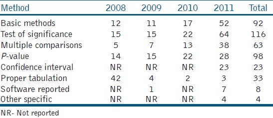
The use of statistics was more in the year 2011, as compared to the previous years. Sixty three (50%) articles used the Analysis of Variance (ANOVA) out of which 47 (74%) articles used multiple comparison tests. The most common mistake in these articles was that 82.8% had not reported the test statistic value and degrees of freedom, and only 17.2% had tabulated the results properly. There was a greater improvement in tabulation and reporting of the confidence intervals in 2011. For multiple comparisons, different tests were used [Table 3] but 10 articles wrongly used the student t-test.

Table 3.

Distribution of proper usage of multiple comparison tests

It should be clear from the above-mentioned findings that using statistics without understanding the principles and the assumptions underlying the tests is a recipe for disaster.

DATA AND ITS REPRESENTATION

The result of any experiment or study is usually documented in numbers. These numbers are nothing but the values recorded for each sample, which talk about the behavior of that sample. As this behavior may differ from sample to sample it is called a variable. The value taken by a variable (shear bond strength, colony count, microleakage) is called data.[4] This data can broadly be classified into Continuous data (Quantitative) and Categorical data (Qualitative) [Table 4]. The most common numerical data dealt with in endodontic literature is continuous data. This data simply means that measurements are made on a scale. There is a possibility of fractions and can often be noted in decimal points. This kind of data is usually summarized as mean ± standard deviation. Categorical data usually divide the samples / specimens / variables into different categories. There can be two or more categories depending on what is measured [Table 4]. This kind of data is usually summarized as frequency (e.g., 3 out of 10 samples had a microleakage score of 4) or percentage (e.g., 30% of the samples had a microleakage score of 4).[4,5] The characteristic is that if the data point is in one class, it cannot be in any other.

Table 4.

Types of data

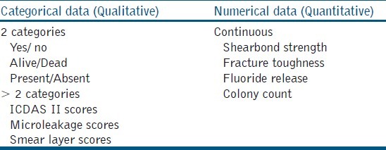
Representation of data is usually done in the form of tables and graphs. Such a representation allows the reader to comprehend the entire essence of the study in one view. Hence, it is imperative to have a complete representation of the variables recorded in a succinct manner. A well-constructed tabular representation allows the reader to understand the results without referring to the text. The following are the essential parts of a table:[4,5]

1. The title should answer the following questions: What does the data present (Mean ± Standard deviation (SD) of shear bond strength), what is the source of the data, the period to which it relates, and the classification used.

2. The unit of measurement of each characteristic presented in the table has to be shown. If only one parameter is measured then this could be included in the title. If there is more than one characteristic, it has to be represented in the corresponding column.

3. The mean and standard deviation or standard error is representative of continuous data. These values are to be represented by not more than one decimal place over the raw data. (e.g., the mean shear bond strength is 7.4 ± 1.2)

4. Categorical data such as disease present or absent is better represented in actual numbers if the sample size is small. It must be noted that half equals 50% and so does 50 / 100. If there are more than two categories, then the groups are described in rows and the categories in columns [Table 5]. It is often noted in endodontic literature that scores are expressed in mean ± SD; which is inappropriate. It must be noted that the statistical methods will differ for averages when compared to those used for percentages.

5. When converting actual numbers of categorical data to percentages; it should be represented to not more than one decimal place.

6. The groups are always represented in rows and it is better to mention the names (Preferably proprietary name) of the groups rather than noting them as group I, group II, and so on [Table 5].

7. P-values are always greater than 0. The computer generated p-values such as P = 0.000, must be written as P < 0.01. It is also a good practice to give the exact P-values that are given by the software. Values such as P = 0.0029 can be rounded off to P = 0.003. When represented in the table, they must be denoted with symbols in degrees of significance, in the footer at the end of the table. Not significant values must also be represented as exact numbers, such as P = 0.2 and not as P = NS.

Table 5.

Microleakage score for three different bonding agents^#

Table 5 depicts the microleakage score for three different bonding agents. Graphical representation of data is a visual method to provide information on quantitative data, which gives a quick comprehension of the facts. It may be furnished as bar diagrams, pie charts, or line diagrams.[4] However, presenting the same information in tables and graphs is not necessary.

MEASURES OF CENTRAL TENDENCY AND DISPERSION

When we collect data pertaining to the study, first-hand documentation is often a set of numbers collected in random order. This is referred to as raw data. The description of the raw data is summarized using values that identify the common value (measures of central tendency) and the amount of scatter (measures of dispersion) of the data. The measure of central tendency is the most representative or typical value for a group.[4] This is given by the mean, median, or mode.

Mean is the arithmetic average of the values of a group. It is affected by extreme values of the group. The mean values have an important effect when the number of samples / observation is more. The median is given by the value of the variable that falls in the central position after arranging the values of a group in ascending or descending order. If there are even numbers of samples / observations in a group, then the median is given by the average of the central two values. The median is usually not affected by the extreme values. The count of a particular observation that occurs more than that of other observations is called a mode. The mean and median are more often used than modes.[4] The computed mean does not usually represent the mean of the samples in a group, but rather a representative mean of the samples of this type.[6] for example, if we aim to determine the shear bond strength of a new bonding agent, then we choose an appropriate methodology to test it; like consider in a class V cavity restoration. The calculated mean shear bond strength 6.3 MPa for a bonding agent is not the bond strength of this bonding agent, but it is the bond strength in this particular scenario. The bond strength may differ with difference in methodology. It is important to note that the mean of the sample is not representative of the property exhibited by the product. Hence, the mean or median alone is not adequate to understand the behavior of the samples in a data set / group. It is important to know the variance of the samples, as much as it is important to know the central value of a data set [Figure 1].

Figure 1.

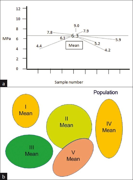
(a) Illustration of shear bond strength values (MPa) of eight samples from a reference population, showing SD, and (b) Repeating the same methodology in different sample sets of the same population, showing SE

There are two types of variance that are used in conjunction with the mean: Variance from the mean and variance of the mean, typically known as Standard deviation and Standard error, respectively.[6] These two terms are most often misunderstood in medical statistics.[7] To simplify; the deviation of individual variables from the mean and from each other is given by Standard Deviation (SD). When SD is expressed as a function of the mean, it completes the information for that data set / group. Mean ± SD is expressed only for continuous data.

To understand standard error, consider this hypothetical situation. If the above-mentioned experiment is repeated with a different set of samples, it cannot be guaranteed that the mean shear bond strength would be exactly 6.3 MPa. The new experiment can yield a mean value of around 6.3 MPa. It can be 6.1 or 6. The measure by which the computed mean would vary if the experiments were repeated is given by the standard error (SE). SD is part of the descriptive statistics, while SE is a part of the inferential statistics. SE is directly affected by the sample size. Hence, for experiments conducted with a smaller sample size, it is preferable to provide Mean ± SE. If the SE is high, then the inference is that the mean obtained with the current study can vary drastically under similar testing conditions with other samples from the same population. SE is a better measure for understanding material science.

NORMAL DISTRIBUTION

This term is often misunderstood as an ideal situation that results of a study should demonstrate. Normal distribution is often erroneously used synonymously with the quality of the study. However, that is not the case for all the hypotheses that need to be tested statistically. To understand normal distribution better, consider a hypothetical experiment where the antimicrobial efficacy of calcium hydroxide medicament against Enterococcus fecalis, in 40 root dentin specimens, is studied, and the colony count is being tabulated. The raw data would be noted as show in Table 6. In order to understand the distribution of this data set, Table 6 could be converted into a frequency (number of specimens in the distribution table, which describes the number of specimens for different ranges of colony forming units [Table 7]. The same is represented in graphs [Figures 2a], which give the frequency of distribution and probability density of distribution, [Figure 2b] respectively.[8] When the density of distribution follows a unimodal, symmetrical, and bell-shaped distribution, it is called normal distribution. This type of distribution is purely affected by the number of observations in each frequency / class interval, which in turn is affected by the sample size. There could be conditions where the distribution could be bi-modal or asymmetric, and such distributions are said to follow Non-normal Distributions. The data is said to be skewed when an otherwise normal distribution has a long tail to the right or the left.

Table 6.

Raw data of colony forming units of E.feacalis following treatment with calcium hydroxide^*

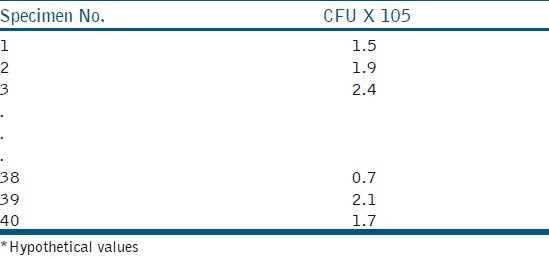
Table 7.

Frequency distribution for data in Table 6

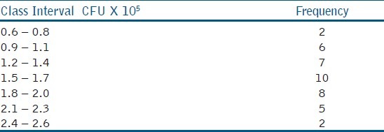
Figure 2.

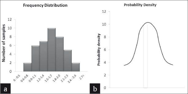
CFU of E.feacalis following treatment with calcium hydroxide described as (a) Frequency distribution and (b) probability density of distribution

Normally distributed data give us the information about the sample mean and SD. If we observe the table, it can be noted that the maximum number of observations is 1.5 – 1.7 × 10⁵, thus indicating the position of the mean (m). The center of this distribution gives the sample mean and on either side of the mean is the dispersion of the remaining values, that is, the SD (σ). For normally distributed data, 95% of the observation will be accommodated between the limits m ±1.96σ and 99% of the observations within m ±2.576σ [Figure 3]. When conducting a study, there is a chance for error and we cannot argue the results with 100% authority. Hence, the allowable error is assumed to be 5% and we tend to summarize the credibility of the results within a 95 % probability. This 5% error by chance gets divided on either side of this bell-shaped curve, beyond m ±1.96σ.

Figure 3.

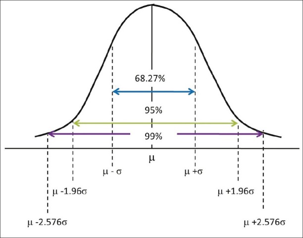
Normal distribution

When the data do not follow normal distribution, then the data can be transformed by taking a logarithm or simply using the statistical methods to test the non-normal data.[8] It is important to note here that the use of the mean along with its SD can be used for statistical analysis only if the sample size is large enough to have a ‘normal distribution’. Normal distribution may serve as a better predictor when the results of a study are to be generalized to the entire population, for example, the longevity of class V composite restoration in treating non-carious cervical lesions (NCCL). However, statistical inference from non-normal data is not obsolete, especially when the results contribute to the understanding of a part of a material or mechanism, and where generalizability to the entire population is not considered; for example, flexural strength of a microfilled composite resin. Here the flexural strength is a part of the mechanical properties, which can indirectly influence the clinical outcome. Hence, if the research question is to test the clinical performance of microfilled composite resin in NCCL, then phase I of the study would be to test the mechanical properties of different composite resins where the sample size is less critical. Phase II of this study would be to narrow down to two to three composite resins from phase I and test them in a clinical trial, where sample size becomes mandatory.

HYPOTHESIS TESTING

How to derive meaningful research questions has been discussed in part I of this review series.[9] Once we have the research question, a hypothesis has to be generated. Statistical tools are so formulated that they disprove a hypothesis rather than prove it. Hence, a study is started by assuming a null hypothesis and later trying to disprove the null hypothesis. Statistical inference consists of two components: Summary statistics and hypothesis testing or inferential statistics.[10] Summary statistics is given by the mean, SD, SE, normal distribution, demographic comparisons, and so on. Disproving the null hypothesis falls under hypothesis testing. Consider an experiment testing the fluoride release of glass ionomer cement (GIC) versus a compomer.

• Research question: Is there a difference in fluoride release between the Compomer and Glass ionomer cement?

• Null Hypothesis: There is no difference in fluoride release between the Compomer and Glass ionomer cement

• Alternate Hypothesis: There is a difference in fluoride release between the Compomer and Glass ionomer cement

We aim to test the fluoride release in a selected sample and this sample is only a representation of the bigger population or the truth. Hence, before testing the hypothesis we need to take a step back and analyze the key components that go into hypothesis testing. As mentioned earlier, any experiment is bound by a set of errors. Let us understand these errors with the help of a decision table [Figure 4]. If the null hypothesis is true and our research finding is also the same, then there is no dilemma. A similar situation exists when both the null hypothesis and research findings appear to be false. If the null hypothesis in actuality is false, that is, the fluoride release is not the same, but our research finding erroneously concludes that the null hypothesis is true, then this type of error is called type II error or b error. This means we can use either GIC or compomer as restorative materials, and the fluoride release is the same. This error is not a serious error and the probability of committing such an error is usually set at, 20 % of the time. If the null hypothesis in actuality is true, that is, the fluoride release is the same, but our research finding erroneously concludes that the null hypothesis is false, then this type of error is called type I error or a error. This means that according to our study, one is more superior to the other, and hence, we will not recommend the material with lesser fluoride release as a restorative material. This is a grave error, as this is a departure from the truth. However, we cannot obviate this error, because we are testing only a representative sample. Hence, this error has to be kept as low as possible and not above 5%. For in-vitro studies, all the testing parameters are under the operator's control, hence this error can be kept as low as 1%. These errors and certain other parameters are to be considered before commencing the study.

Figure 4.

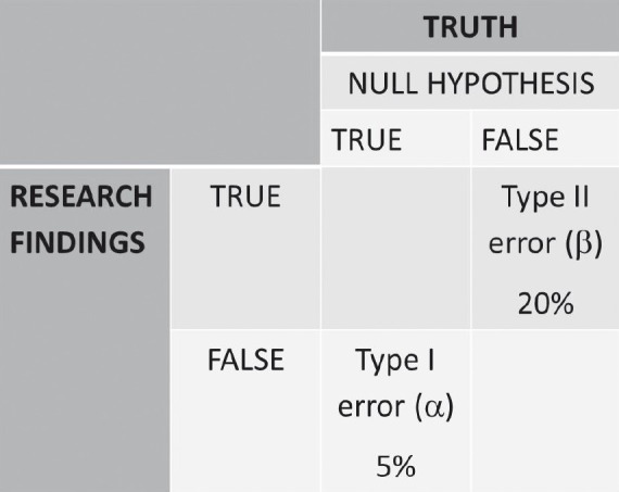
Decision table in understanding errors associated with experimental study

Having understood this, let us presume to have completed the experiment considering all the parameters that would affect the outcome of the study. Assuming that the data sets of both the GIC and compomer follow a normal distribution, their representation would be similar to Figure 5a. If the distributions do not overlap [Figure 5b] then the inference is direct that both groups are different. If the distributions of both groups grossly overlap [Figure 5c], again the inference is direct that the groups are similar. These are hypothetical situations [Figures 5b and c] and experiments do not follow this trend. The dilemma arises when the distributions overlap on a very minimal scale [Figure 5d]. In statistical hypothesis testing what is measured is, if the overlap occurs on the tail end of distributions comprising of < 5% of the observations of both groups, then the groups are declared to be significantly different. The overlap of distributions is considered to have occurred by chance and this overlap of chance has already been accounted for while calculating the sample size as an a error. This forms the basis of setting the P-value or the probability value at < 5% or popularly termed as P < 0.05.

Figure 5a.

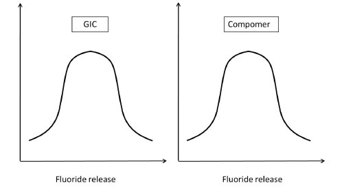
Fluoride release of GIC and Compomer

Figure 5b.

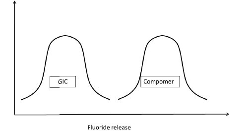
Fluoride release of GIC and Compomer Comparison of Fluoride release of GIC and Compomer

Figure 5c.

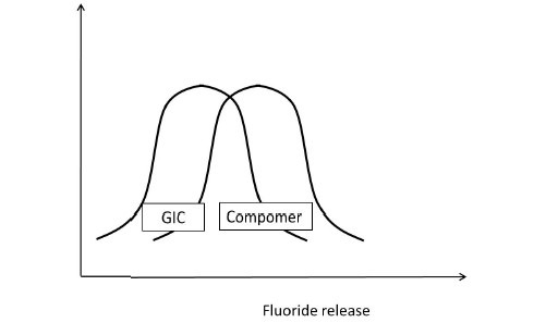
Comparison of Fluoride release of GIC and Compomer

Figure 5d.

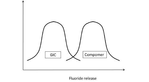
Comparison of Fluoride release of GIC and Compomer

However, statistical significance is not the benchmark to derive conclusions in a study. Clinical significance is not always synonymous with statistical significance and the judgment lies in the cognitive deduction of the facts with knowledge and clinical expertise.

SAMPLE SIZE

In statistics, we usually compare two groups or samples. Even when we study only one sample, our aim is to state whether this sample is similar to or different from the population from which it is drawn. A sample is a group of people selected from a larger group of people. What do we study? We have seen that there are several types of research questions, and each of these is based on a unique hypothesis. Thus, the estimate we get from the study for each kind of question is a unique kind of estimate; examples are: Difference in means, proportions, odds or risk ratios, prevalence or incidence, and so on. It is intuitive that the number of people we need to see in order to get ‘believable’ estimates for each of these is different. This is the basis of sample size calculation.

In order to calculate a sample size, we need to know the following: What is the level of alpha error and beta error that we are prepared to accept? That is, to what extent are we prepared to accept that our result could be a chance finding? That this chance has to be minimal is intuitive. Conventionally, people accept 5% for type 1 error and 20% for type 2 error. Second, What is the present level of or rate of occurrence of the event we are interested in? That is, what is the cure rate without the new intervention? Third, What is the extent to which we want to modify this? That is, what is the clinically meaningful difference? Needless to say, the investigator has to specify this. Then the number of subjects that need to be studied can be calculated using different formulas.

Different questions have to be answered by different study designs. The data collected can be continuous or categorical. Thus, the method of calculating sample size will differ with each study design and will be discussed in detail while addressing those designs.

STATISTICAL METHODS

Reflecting on the review of articles that were evaluated for statistical methods, the Kruskal Wallis test or ANOVA for comparing two groups was used in seven articles, which is not correct. In the year 2011, advanced statistical method survival analyses were found in three articles. About 10 articles reported in the abstract, but it was not found in the full article and eight articles reported the P-value, but not the statistical methods.

The choice of the comparison procedure will depend on the exact situation and it is more important to keep a strict control over the groupwise error rate and to have greater statistical power [Figure 6a and b]. When there are equal sample sizes in the groups and when population variances are similar, then the Bonferroni test could be used for a smaller number of comparisons (< 5) and in case of more than five (> 5), it is preferred to use the Tukey test, as both have good power and control over the Type I error rate. When the sample sizes and population variances differ between groups, it is proven that the Games-Howell and Dunett's tests give the accurate result, and SPSS provides all these test options. When multiple t tests are used for comparison then there is no attempt to control the Type I error. Before using ANOVA and multiple comparison tests, the Kolmogrov-Smirnov Test (Test for normality) and Levene test (Homogeneity of Variances), it should be reported in the article. Hence, it is always advised to have a prior consultation with a statistician to match the data, analysis, and conclusions.

Figure 6.

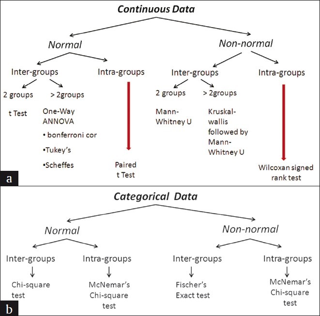
Statistical Methods. (a) Continuous Data (b) Categorical Data

CONCLUSION

The results section of a study is the lifeline of any original research. It is the responsibility of the investigators to understand this section in order to bring out a meaningful inference. Statistics is the only method available to deduce this inference. Hence, our understanding of the statistical methods plays a pivotal role in claiming authority of the inference of our study.

REFERENCES

- 1.Platt JR. Strong inference. Science. 1964;146:347–53. doi: 10.1126/science.146.3642.347. [DOI] [PubMed] [Google Scholar]
- 2.Krasner, Rankow Anatomy of the pulp-chamber floor. J Endod. 2004;30:5–16. doi: 10.1097/00004770-200401000-00002. [DOI] [PubMed] [Google Scholar]
- 3.Vähänikkilä H, Nieminen P, Miettunen J, Larmas M. Use of statistical methods in dental research: Comparison of four dental journals during a 10-year period. Acta Odontol Scand. 2009;67:206–11. doi: 10.1080/00016350902837922. [DOI] [PubMed] [Google Scholar]
- 4.Jayaseelan L, Kavitha ML. Types and presentation of data, normality, variance and confidence interval. Peadiatr Today. 2001;4:407–13. [Google Scholar]
- 5.Altman DG, Bland JM. Presentation of numerical data. Br Med J. 1996;312:572. doi: 10.1136/bmj.312.7030.572. [DOI] [PMC free article] [PubMed] [Google Scholar]
- 6.Altman DG, Bland JM. Statistical notes: Standard deviations and standard errors. Br Med J. 2005;331:903. doi: 10.1136/bmj.331.7521.903. [DOI] [PMC free article] [PubMed] [Google Scholar]
- 7.Nagele P. Misuse of standard error of the mean (SEM) when reporting variability of a sample. A critical evaluation of four anaesthesia journals. Br J Anaesthesiol. 2003;90:514–6. doi: 10.1093/bja/aeg087. [DOI] [PubMed] [Google Scholar]
- 8.Altman DG, Bland MJ. The normal distribution. Br Med J. 1995;310:298. doi: 10.1136/bmj.310.6975.298. [DOI] [PMC free article] [PubMed] [Google Scholar]
- 9.Krithikadatta J. Research methodology in dentistry. Part I – The essentials and relevance of research. J Conserv Dent. 2011;15:5–11. doi: 10.4103/0972-0707.92598. [DOI] [PMC free article] [PubMed] [Google Scholar]
- 10.Zou KH, Fielding JR, Silverman SG, Tempany CM. Hypothesis testing I: Proportions. Radiology. 2003;226:609–13. doi: 10.1148/radiol.2263011500. [DOI] [PubMed] [Google Scholar]