

Abstract
The monkey’s auditory cortex includes a core region on the supratemporal plane (STP) made up of the tonotopically organized areas A1, R, and RT, together with a surrounding belt and a lateral parabelt region. The functional studies that yielded the tonotopic maps and corroborated the anatomical division into core, belt, and parabelt typically used low-amplitude pure tones that were often restricted to threshold-level intensities. Here we used functional magnetic resonance imaging in awake rhesus monkeys to determine whether, and if so how, the tonotopic maps and the pattern of activation in core, belt, and parabelt are affected by systematic changes in sound intensity. Blood oxygenation level-dependent (BOLD) responses to groups of low- and high-frequency pure tones 3-4 octaves apart were measured at multiple sound intensity levels. The results revealed tonotopic maps in the auditory core that reversed at the putative areal boundaries between A1 and R and between R and RT. Although these reversals of the tonotopic representations were present at all intensity levels, the lateral spread of activation depended on sound amplitude, with increasing recruitment of the adjacent belt areas as the intensities increased. Tonotopic organization along the STP was also evident in frequency-specific deactivation (i.e. “negative BOLD”), an effect that was intensity-specific as well. Regions of positive and negative BOLD were spatially interleaved, possibly reflecting lateral inhibition of high frequency areas during activation of adjacent low frequency areas, and vice versa. These results, which demonstrate the strong influence of tonal amplitude on activation levels, identify sound intensity as an important adjunct parameter for mapping the functional architecture of auditory cortex.
Introduction
Tonotopic representation is a salient organizing principle of mammalian auditory cortex. In the macaque monkey, neurons on the supratemporal plane (STP) respond to auditory tones, with many of them displaying clear preferences for a narrow range of stimulation frequencies. Most notably, the core region receiving direct input from the ventral division of the medial geniculate nucleus shows a strong tonotopic organization, as demonstrated by numerous single unit studies. Within the core, neurons have preferred or characteristic frequencies (CF), which progress along the caudorostral axis. Reversals in this progression serve as a basis for dividing the auditory core into distinct functional subdivisions (A1, R, and RT), each of which represents a full complement of low to high frequencies (Merzenich and Brugge, 1973); (Morel et al., 1993); (Recanzone et al., 2000); (Kaas and Hackett, 2000)). The auditory core sends projections to a surrounding belt of second order areas, which send projections, in turn, to a large laterally adjacent, higher order parabelt region on the lateral surface of the superior temporal cortex. A recent functional magnetic resonance imaging (fMRI) study in monkeys (Petkov et al., 2006) that applied tonotopic mapping succeeded in demonstrating several of these subdivisions simultaneously.
Auditory mapping has traditionally relied on measuring the responses of single neurons to the presentation of threshold-level tones, with a given neuron’s CF defined as the frequency requiring the lowest sound intensity level to elicit a response. Given the standard of mapping with low intensity stimuli, the relationship of tonotopic maps to normal auditory processing is unclear, as CF maps do not indicate the acoustic frequencies that neurons will respond to if the stimuli are presented at suprathreshold intensities. Might tonotopic maps measured with fMRI change as a function of sound intensity? Might different stimulus intensities serve as a means of identifying the spatial boundaries between auditory subfields?
To explore these questions, we performed fMRI in awake macaque monkeys while systematically varying sound levels of the tonal stimuli. Human fMRI studies have reported that increasing sound levels result in a spread of activation over the auditory cortex (Jäncke et al., 1998); (Hart et al., 2003). However, spatial resolution in most previous studies was not high enough to allow identification of auditory subdivisions, and the basis of this spread is therefore unclear. Other, higher resolution studies showing tonotopic maps in humans have not varied the sound level (Formisano et al., 2003). In the present study, mapping was conducted using mixed tone stimuli in two different frequency ranges, presented at three distinct sound intensity levels through calibrated headphones. We observed dissociable effects of frequency and intensity in the spatial pattern of activation, suggesting that fMRI intensity tuning, together with frequency tuning, might serve as a basis for functionally dividing auditory subareas.
Materials and Methods
Subjects
The subjects were two rhesus monkeys (Macaca mulatta), a female (M1) weighing 4.8 kg, and a male (M2) weighing 8.5 kg. Three hemispheres were studied — left and right hemispheres separately in M1, and the left hemisphere in M2. All procedures were carried out in accordance with the Institute of Laboratory Animal Resources Guide for the Care and Use of Laboratory Animals and were approved by the Animal Care and Use Committee of the National Institute of Mental Health.
The monkeys’ hearing ability between 892 and 7996 Hz as well as middle ear function of both monkeys were tested on multiple occasions by audiologists using distortion product otoacoustic emission (DPOAE). To determine optimal settings and MR parameters, we presented pure tones at different frequencies to the right ear of M1 during ~30 scanning sessions. The audiological results showed normal function before and after both the optimization sessions and full data acquisition.
Training
The animals were first acclimated to a monkey chair and then trained in a mock-MRI setup in which they performed a visual fixation task for about 2 hours/day. During this training a recording of the MR gradient noise was played continuously in the background. The monkeys then underwent a period of acclimation to the scanner during which they received repeated MR scans with auditory stimulus presentations. Fixation training was suspended at this time so that their eyes could be carefully monitored with an infrared eye-camera in order to assess their reactions to the stimuli and overall behavioral state. Once they adapted to this environment, they typically sat quietly but tended to do so with eyes closed despite the gradient noise; also, importantly, they showed no particular response to the presentation of the pure tones, regardless of the changes in acoustic frequency and intensity. Therefore, in order to reduce the opportunity for postural- and eye-movement artifact, we chose to use passive listening without fixation during the formal sessions in which fMRI data were acquired for later analysis.
Sound presentation
Sounds were presented from a Windows PC using Adobe Audition, amplified with a power amplifier (Gemini P07), and delivered from an electrostatic ear-speaker (STAX SR-003) mounted on an ear mold that was custom made for each monkey (Starkey Eden Prairie, MN). The speaker was placed on the ear contralateral to the hemisphere being studied, while the other ear was occluded with a silicone earplug (Insta-Putty, Insta-Mold Products, Inc., Oaks, PA).
Acoustic calibration
Prior to each session, acoustic calibration was performed in the ear canal with a sound-level meter (Larson Davis model 800B) and a preamplifier (Larson Davis PRM 826B) with a probe microphone (Bruel & Kjaer type 4182) inserted in a vent drilled through the ear mold. Calibration was performed using root mean square (RMS) matched pure tones interspaced every 1/3 octave. The frequency response of the ear speaker was flattened (+/− 6 dB, A-weighting) at each of 6 pure tones (0.6-7 kHz) by a graphic equalizer (Yamaha Q2031B). For higher tones between 10 and 14 kHz, calibration was performed using a 10 kHz pure tone.
Stimuli
Two sets of four pure tones several octaves apart were presented separately in interleaved runs of acquisition. For the left hemisphere of M1, the first hemisphere studied, the two sets of tones were separated by a 4-octave interval, with the low frequencies ranging from 0.6 to 0.9 kHz, and the high frequencies, from 10 to14 kHz. Because analysis of the results indicated there was sufficient spatial resolution in the scans to differentiate a narrower interval between the two set of tones, the interval for the next two hemispheres studied (M1 right and M2 left) was reduced to three octaves, with the low-frequency range as before but with the high frequency range reduced to 5-7 kHz. Each tone had a duration of 200 msec (rise and fall time, 10 msec each) interspaced by 50 msec of silence. A single run lasted 864 sec to collect 432 MRI time points. Each set of four tones was presented in 24-sec blocks at 3 different sound levels — 70, 80, and 90 dB SPL (except for the high pure tones used to study the left hemisphere of M1, which were presented at 70, 75, and 80 dB SPL). Each run contained 18 blocks of sound stimulation (6 blocks at each of the 3 sound levels) separated by 24-sec interblock silent periods. Runs with low tones and high tones were repeated three times each in one session, and each session lasted 2-3 hours, including preparation scans.
MRI equipment and data acquisition
Functional images were acquired in a 4.7T Bruker vertical scanner. Volumes with 7-9 slices were acquired with a single-shot EPI sequence (TE/TR, 25/2000 msec; field of view (FOV), 128 × 96 mm; matrix size, 128 × 66; slice thickness, 1.5mm; flip angle, 75 degrees). Custom-made transmitter/receiver surface coils with diameters of 30 mm (for M1) and 50 mm (for M2) were located above and contralateral to the ear to which the sound was presented. Anatomical scans were obtained with a MDEFT sequence (TE/TR, 13.9/4.55 msec; FOV, 128 × 112 mm; matrix size, 256 × 224). For each hemisphere studied, care was taken to reproduce the same slice configuration in every fMRI session. This was facilitated by the fact that the angle of the headpost in relation to the headpost holder was fixed, and the height of the oblique axial slices could be matched across sessions by reference to blood vessels on the STP. To obtain a rough measure of the quality of the MR signal, the signal to noise ratio (SNR) of the first run in a session was calculated for each day’s session by dividing the mean signal strength on the STP by the mean standard deviation value of the voxels in the background. The SNR range (mean) for the three hemispheres was as follows. M1 right: 218-307 (275), M1 left: 193-361 (300), M2 left: 143-175 (164). The lower SNR in M2 than in M1 is likely due at least in part to M2’s larger size (see Subjects); i.e. his larger temporalis muscle required a larger diameter surface coil (see above), resulting in the lower SNR.
fMRI data analysis
After volume acquisition, timepoints with outliers (approximately 20% of all timepoints) were detected by visual inspection guided by the AFNI (http://afni.nimh.nih.gov/afni/) program ’3dToutcount’ and removed from the analysis. Acquired volumes were volume registered to an average volume of a first run, and then normalized to the mean MRI signal. Data from 4 sessions (3 runs each) were aligned using the AFNI program ’3dTagalign’, concatenated, and subjected to multiple linear regression analysis. Voxels outside the brain were masked out. Regressors were created by convolving a boxcar design matrix with a gamma function. Twelve motion profiles derived from volume registration were incorporated into a general linear model as regressors of no interest. No spatial smoothing was applied. The EPI and anatomical scans were aligned using the AFNI program ’3dTagalign’. To obtain a ’collapsed map’, a maximum projection of the t-map was taken across 4 slices each for high and low frequency tones (HFT and LFT, respectively), then separate colors were assigned to HFT and LFT (red and green, respectively), and finally the two different frequency maps were overlaid. Using the AFNI program ’AlphaSim’, we applied small volume correction for multiple comparisons with Monte Carlo simulations. The spatial correlation of the input data and an uncorrected p value threshold of 0.0001 (t = 3.89) determined the minimum cluster size of 3 voxels to achieve a corrected p value of < 0.05. The number of voxels on the STP that fulfilled this criterion was counted for each intensity and each tone. In thresholded maps, threshold was accordingly set at t = 3.89. The mean percent signal change from the baseline for each of 5 regions of interest (ROI) was calculated based on the GLM analysis in M1’s right hemisphere and for each of 4 ROIs in M1’s left hemisphere. The ROI was defined as clusters of contiguous voxels with absolute t-value exceeding the threshold of 3.89 for at least one intensity level (Fig. 6c).
Figure 6.

The percent signal change in response to HFT for each ROI in M1 right hemisphere and M1 left hemisphere. a) Percent signal change was monotonically modulated in proportion to sound intensities in ROI 1-4 but not in ROI 5. b) Monotonic percent signal change was seen in ROI 1 and 3 but not in 2 and 4. c) d) ‘collapsed map’ of ROIs in M1 right and M1 left, respectively. Based on the tonotopic representation, ROIs 1/2 include AI, 2/3 include R, 3/4 include RT, and 4/5 include unknown rostral area.
Results
Functional data were collected in oblique axial slices parallel to the STP throughout the study (Fig. 1a). Low frequency tone (LFT) and high frequency tone (HFT) stimuli elicited alternating zones of positive and negative activation relative to baseline, as can be seen in the raw activation maps (t-maps) from one hemisphere (Fig. 1b). Focusing first on the positive activation, we observed interleaved regions of high and low frequency maximal responsiveness, spanning roughly 2 cm in the rostrocaudal direction. Fig. 2 shows this activation pattern for each of the three hemispheres tested. Based on the tonotopic transitions, approximate subdivisions of the auditory core (A1, R, and RT) were estimated; these match previous descriptions of the tonotopic organization of macaque STP (Merzenich and Brugge, 1973; Petkov et al., 2006).
Figure 1.

Orientation of oblique axial brain slices and raw activation. a) The configuration of slices parallel to the lateral sulcus used in this study. b) Unthresholded activation map (t-map) on the STP of the right hemisphere of M1 at 80dB. Activation clusters (positive BOLD) are shown in dark red, and deactivation clusters (negative BOLD), in dark blue. Abbreviations: LFT, low frequency tones; HFT, high frequency tones. Scale bar, 10 mm. In each slice, caudal is downward and medial is to the left.
Figure 2.

Maximum projection map of the tonotopic representations in each hemisphere — M1 right, M1 left, and M2 left. Maps were derived from positive BOLD responses at 80 dB (M1 left, HFT at 75dB) collapsed across 4 slices through the depth of the STP and thresholded at t = 3.89. Areas activated by high and low frequency tones are shown in red and green, respectively; overlap between the two in M1 right is shown in yellow. The long dotted arc on each collapsed slice marks the lateral edge of the STP, and the short dotted arc marks the circular sulcus, which forms the medial edge of rostral STP. Positions of A1, R, and RT were estimated based on mirror reversals of the tonotopic representations: high to low in A1, low to high in R, and high to low again in RT. Abbreviations: H, high frequency tones; L, low frequency tones. Scale bar, 5 mm.
The maps in Figs. 1 and 2 were collected with sound intensity levels of 80 dB. Notably, the scanner noise associated with continual fMRI sampling did not pose an obstacle for evaluating tonotopic maps in the brain. We next asked whether the structure of these maps had been influenced by the sound pressure level at which the tones were delivered. The raw maps in Fig. 3 (M1 right hemisphere) and S Fig. 1 (M1 left and M2 left) show that the spatial pattern of activation was strongly influenced by the sound intensity level, with each of the test levels well above the monkey’s hearing threshold. First, in terms of the number of activated voxels (threshold = t > 3.89), the highest intensity tones showed wider activation by a factor of more than 3:1 (Fig. 4). The overall spatial extent of activation was largest for 90 dB stimuli compared to 80 and 70 dB for both high and low frequency stimulation. Second, changes were observed among voxels modulated in both directions (i.e. positive and negative BOLD). Note that the negative BOLD modulation was consistently seen in both hemispheres of M1 (Fig. 3 and S Fig. 1a). Its spatial alternation with the positive BOLD resembled that of the areal tonotopy itself, with some areas that showed positive BOLD in response to high tones showing negative BOLD in response to low tones, and vice versa (Fig. 5). As to the modulation of the positive BOLD, the analysis in Fig. 6 revealed monotonic responses to sound intensity except that the rostralmost aspect showed nonmonotonic responses. The effect of sound intensity on negative BOLD modulation varied between hemispheres (Fig. 3, Fig. 6).
Figure 3.

Unthresholded t-map at each sound intensity in M1 right hemisphere. Note increasing spread of activation at the higher stimulus intensities.
Figure 4.

The numbers of voxels that survived the threshold of t > 3.89 and cluster size larger than 3 for each tone and sound level. A, M1 right hemisphere; B, M1 left hemisphere; C, M2 left hemisphere; HFT, high frequency tones; LFT, low frequency tones.
Figure 5.

Three perpendicularly oriented views of the thresholded map (t > 3.89) of M1’s right hemisphere in response to 80 dB HFT and LFT overlaid on a high-resolution anatomical scan of this hemisphere. Oblique axial sections (a, e), sagittal sections (b, f), and oblique coronal sections (c, d). Horizontal green lines in (a) and (e) indicate location of coronal sections 1-6. Vertical green lines in (a) and (e) indicate location of sagittal sections. Note that areas activated by high tones tend to be deactivated by low tones, and vice versa. Scale bar, 5 mm.
The maps in Fig. 7 show the effect of sound intensity level on the tonotopy of the STP. The tonotopic transitions were consistent across intensities (Fig. 7a). Note that activation at the 70 dB level is largely restricted to the auditory core itself, based on known anatomical and previous mapping studies. In contrast, activation at the higher levels shows considerable activation of the surrounding belt regions (Fig. 7a,b).
Figure 7.

Effect of sound intensity on spatial spread of tonotopic maps. a) Maximum projection maps of the tonotopic representations as in Figure 2, at multiple intensities. Note the small, rostralmost cluster in M1’s right hemisphere denoting a high frequency representation at all sound levels (arrows). b) Estimates of the auditory core and belt subdivisions based on the activation patterns shown in a). Outlined area marked with ’?’ in M1’s right hemisphere is potentially a 4th tonotopic subdivision located rostral to the auditory core. Abbreviations: H, high frequency tones; L, low frequency tones; LB, lateral belt; MB, medial belt. Scale bar, 5 mm.
In each hemisphere, the maximum sound intensity led to a spatial activation pattern that was between 10-15 mm in width, exceeding the typical core’s width of ~5 mm (e.g. Kosaki et al., 1997; Hackett et al., 2001). Interestingly, whereas the spread of activation to high intensity HFTs in field A1 was observed medially, laterally, and caudally, the rostral boundary of the activation was invariant for sound levels between 70 and 90 dB. The findings confirm that tonotopic segregation extends into the belt (Rauschecker et al., 1995; Petkov et al., 2006), with local frequency preferences generally being continuous with those in the adjacent core area (see Fig. 8). Based on these observations, we conclude that areas within the auditory belt are recruited in a frequency-specific manner at higher intensity levels. The other finding of note is a rostral zone of high frequency activation observed in M1’s right hemisphere (Fig. 7a, arrow); although the size of this zone was small, its activation was reproducible across intensities and across sessions (S Fig. 2).
Figure 8.
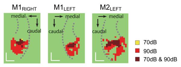
Clusters in the maximum projection map (Fig. 2) of putative A1 and surrounding belt areas in response to high frequency tones presented at 70 dB and 90 dB (80dB in M1 left) plotted separately and together. Spread of activation in all directions except rostrally was prominent in each hemisphere as the sound level increased. Note that only a single voxel (M1 right) was activated at 70 dB but not at 90 dB. Scale bar, 5 mm. (For further description, see legend to Fig. 2.)
Discussion
Frequency-based encoding is a fundamental principle of the auditory system, beginning with the spatial ordering of frequency selectivity along the cochlea. Each of the subdivisions of the core area of the auditory cortex receiving input from the ventral subdivision of the medial geniculate nucleus of the thalamus maintains this tonotopic organization. The present findings use BOLD fMRI in unanesthetized rhesus monkeys to examine tonotopic organization of the auditory cortex at different intensities of the pure tones. The spatial extent of tonotopic maps was strongly influenced by the sound intensity level, with the higher intensities causing a lateral spread of activation in a frequency-specific manner from the auditory core into both medial and lateral belt regions of the supratemporal plane.
Cortical representation of frequency and intensity
Like selectivity for frequency, that for intensity level may serve as an organizing principle of auditory cortex. Human fMRI studies varying this parameter have reported the monotonic spread of activation when the sound intensity level is increased (Jäncke et al., 1998; Hart et al., 2003). One study reported a drift in the locus of activation, suggestive of ampliotopic coding, i.e. spatial activation patterns tied to the amplitude of the sound stimulus (Bilecen et al., 2002). The cortical mechanisms of intensity-dependent variation in activation patterns have been a topic of debate. At the cellular level there are at least two possible mechanisms (Brechmann et al., 2002) by which increasing sound pressure level could alter the spatial pattern of responses. First, neurons in neighboring cortical areas with lower sensitivity to sound pressure level, but with monotonic sensitivity functions, might become activated, resulting in a spread of activation (i.e. recruitment within a tonotopic map). Second, increasing the sound intensity may activate adjacent cortical regions while simultaneously inactivating those responsive to the lower sound intensity, a consequence of nonmonotonic intensity tuning (i.e. ampliotopic coding).
To date, only two electrophysiological studies have directly evaluated the spatial modulation of the neuronal population response with pure tones at multiple fixed intensities. In one study (Phillips et al., 1994), conducted in anesthetized cats, clusters of nonmonotonic neurons responded only to low intensity tones (20-40 dB), but were unresponsive to high intensity tones (80 dB), resulting in an apparent topographic shift in activity. This finding supports the notion of ampliotopic coding. However, in a study in A1 of awake monkeys, the cortical spread of neuronal activation was proportional to the sound intensity level (B. H. Scott, personal communication). This spread did not affect the characteristic frequencies for the neurons tested within A1 even at the highest intensity tested (80 dB), and therefore does not lend support to the ampliotopic-coding hypothesis.
In the present study, we found no evidence for ampliotopic coding in A1. Higher sound intensity resulted in a spread of activity away from existing peaks, but not a shift in the peak itself or in any other aspect of the tonotopy elicited with the low intensity stimulus. For example, the rostral boundary of the high-frequency representation of A1 in Fig. 8 was largely invariant across intensities. Consistent with the findings of Scott (cited above), the activation patterns elicited by the two frequency ranges were complementary even at the highest intensity (Fig. 7). This is also consistent with studies in which suprathreshold mapping was performed at a fixed intensity of 60-65dB within AI (Fu et al., 2004; Kayser et al., 2008). The spread of activation was directed mainly toward the lateral and caudomedial belt areas, in agreement with the higher neural response thresholds for pure tones in these areas (Kosaki et al., 1997; Recanzone et al., 2000). The present results thus suggest that belt areas can be localized, or at least estimated, with fMRI based on their selective activation to high sound intensity.
A similar trend was seen in the rostral subareas R and RT of the auditory core. In these areas, higher stimulus intensities also elicited a spread of activation primarily in the medial and lateral directions, an effect that was most pronounced for the low frequency tones. An unexpected third cluster selective to high frequency tones was reproducibly observed at the rostral end of the activated region in one monkey (see Fig. 7), suggesting another mirror reversal and possibly a fourth tonotopic representation. Of note is that the sound-level-dependent modulation was less clear in this area (Fig. 6), a finding that may suggest homology to the rostralmost auditory area T1a in humans, which also shows intensity-level-independent responses (Brechmann et al., 2002). The position of this area also suggests that it might correspond to a recently described area outside the core that was reported to be selective for monkey vocalizations (Petkov et al., 2008).
Although, as noted earlier, we did not observe any systematic lid or eye movement in response to the sound presentation, the lack of behavioral control over the subjects’ eye position might raise concern, as it has been shown that eye position modulates neuronal activity in the auditory cortex (Fu et al., 2004). However, this modulation, which takes the form of auditory response enhancement, was reported to occur most commonly during central fixation, regardless of the location of the sound source. Since our monkeys’ eyes were normally closed, and since the tonotopy we observed was comparable to that seen in animals scanned while fixating centrally (Petkov et al., 2006), we assume that eye-position effects on the fMRI signal, if any, were relatively minor ones.
Negative BOLD
In two of the three hemispheres studied, we observed patterns of decreased activation that were both frequency and sound-level specific (e.g. Fig. 3, S Fig. 1). Recent work in the visual system has shown that regions of V1 retinotopically adjacent to stimulated cortex show an apparent decrease in activation, sometimes termed “negative BOLD”. Although the origins of the negative BOLD response are likely to be complex (Harel et al., 2002; Shmuel et al., 2002)), evidence from the visual system studies suggest that it is accompanied by a significant decrease in neuronal activity in the affected cortical tissue (Shmuel et al., 2006). In the present study, regions of positive and negative BOLD were interleaved spatially, corresponding to complementary regions of frequency specificity. This pattern is in good agreement with previous studies of visual cortex activation using checkerboard patterns (Saad et al., 2001; Shmuel et al., 2006). It is possible that the negative BOLD we observed is a consequence of lateral inhibition from adjacent areas that were highly activated by the tonal frequencies to which they were closely tuned.
Unfortunately, lateral inhibition in auditory cortex is not yet well understood, mainly because, until recently, most electrophysiological experiments were carried out in anesthetized animals with suppressed baseline activity. However, recent studies in awake monkeys (Fu et al., 2004; Lakatos et al., 2005) showed that multiunit activity was decreased below baseline in response to pure tones with frequencies surrounding the best frequency for the units being recorded. This observation and ours are both compatible with the existence of frequency- and intensity-dependent surround inhibition (Calford and Semple, 1995) at the population level. Interestingly, although ours is the first explicit report of a negative BOLD response in an auditory study, a similar deactivation can be seen in Figure 3 of the study by Petkov and colleagues (2006), in which a decrease in activity compared to baseline is illustrated in a ‘low frequency area’ in response to high frequency tones. Finally, it is worth noting that in fMRI studies of the visual system, the absolute intensity of a negative BOLD signal is typically much smaller than that of a positive BOLD signal (Harel et al., 2002). Therefore, visualizing negative BOLD requires a high signal to noise ratio (SNR), which presumably explains why negative BOLD was not obvious in monkey M2, in which the SNR was lower than in monkey M1. Given the potential utility of negative BOLD as a marker of population-level surround inhibition, the phenomenon clearly merits further study.
The issue of gradient noise (continuous vs. sparse fMRI sampling)
In the present study, functional volumes were collected at short (2 s) intervals. The acoustic noise caused by the switching of the gradient coil (see S Fig. 3) was continually present in the background. A number of previous studies have considered the adverse effects of gradient noise on auditory studies (Bandettini et al., 1998; Gaab et al., 2007; Schmidt et al., 2008). To prevent contamination of the experimental data by the immediately preceding activation of the coil, ’sparse sampling’ (i.e. lengthening the interval between volume acquisitions) has become the preferred solution. However, it is likely that the choice of the best paradigm is situation-dependent. The mere presence of the noise might not necessarily be deleterious. Seifritz and colleagues (2006) developed an fMRI sequence in a 1.5T scanner that produces a perceptually continuous acoustic noise, which proved to be advantageous in that it allowed demonstration of the mirror symmetric pattern of tonotopic representation not seen with conventional 1.5T scanning. Also, the adverse effect of gradient noise depends on the spectral overlap with the auditory stimuli (Scarff et al., 2004). Our result is consistent with this conditional relationship. Specifically, at an SPL of 70 dB, the low frequency tones (600-900 Hz), which surrounded the spectral peak of the gradient noise (775 Hz), activated a very small area. However, the attenuation was much less marked (if it was present at all) at high intensities of the low frequency tones or at low intensities of the high frequency tones (5-7 and 10-14 kHz), where the gradient noise did not have a major energy spectrum. Tonotopic maps observed in our study with a short TR are consistent with the maps obtained with sparse sampling (Petkov et al., 2006). Our findings thus indicate that tonotopically specific activation can be obtained in the presence of the gradient noise without the use of sparse sampling.
In sum, the present findings affirm that fMRI is a powerful technique for mapping auditory cortex in the monkey and a valuable one in allowing direct comparison with findings in humans. Although the extent of activation varied dynamically in response to multiple sound levels, the tonotopic map visualized with fMRI at suprathreshold intensities largely resembled those obtained by the CF method, i.e. at threshold. However, our results also show that manipulating sound levels can be used to identify subdivisions of the auditory belt and distinguish these from core areas, and is therefore an important adjunct to tonotopic mapping.
Supplementary Material
Supplementary Figure 1. Unthresholded t-maps in (a) M1 left hemisphere and (b) M2 left hemisphere. (For explanation of figure, see legend to Fig. 1b.)
Supplementary Figure 2. Activation maps from six consecutive sessions in which the right hemisphere of M1 was stimulated with high frequency tones at 80 dB. The patterns of activation and deactivation were highly consistent across intersession intervals varying from 7 to 49 days. Scale bar, 10 mm. (For further explanation, see legend to Fig. 1.)
Supplementary Figure 3. Frequency spectrum of the gradient noise. The highest peak was seen at 775 Hz (normalized to 0 dB at 1 kHz). Horizontal bars indicate spectral extent of the low and high frequency tones (LFTs and HFTs, respectively).
Acknowledgement
The authors thank Brian Scott for valuable comments on the manuscript, and Kelly King, Chris Zalewski, Carmen Brewer, Chris Petkov, Chris Kayser, Helmut Merkle, Michael Schmidt, Neal Phipps, Michael Ortiz, Ziad Saad, and Rick Reynolds for valuable advice and technical assistance.
Footnotes
Publisher's Disclaimer: This is a PDF file of an unedited manuscript that has been accepted for publication. As a service to our customers we are providing this early version of the manuscript. The manuscript will undergo copyediting, typesetting, and review of the resulting proof before it is published in its final citable form. Please note that during the production process errors may be discovered which could affect the content, and all legal disclaimers that apply to the journal pertain.
References
- Bandettini PA, Jesmanowicz A, Van Kylen J, Birn RM, Hyde JS. Functional MRI of brain activation induced by scanner acoustic noise. Magn Reson Med. 1998;39:410–416. doi: 10.1002/mrm.1910390311. [DOI] [PubMed] [Google Scholar]
- Bilecen D, Seifritz E, Scheffler K, Henning J, Schulte A. Amplitopicity of the human auditory cortex: an fMRI study. NeuroImage. 2002;17:710–718. [PubMed] [Google Scholar]
- Brechmann A, Baumgart F, Scheich H. Sound-Level-Dependent Representation of Frequency Modulations in Human Auditory Cortex: A Low-Noise fMRI Study. J Neurophysiol. 2002;87:423–433. doi: 10.1152/jn.00187.2001. [DOI] [PubMed] [Google Scholar]
- Calford MB, Semple MN. Monaural inhibition in cat auditory cortex. J Neurophysiol. 1995;73:1876–1891. doi: 10.1152/jn.1995.73.5.1876. [DOI] [PubMed] [Google Scholar]
- Formisano E, Kim DS, Di Salle F, van de Moortele PF, Ugurbil K, Goebel R. Mirror-symmetric tonotopic maps in human primary auditory cortex. Neuron. 2003;40:859–869. doi: 10.1016/s0896-6273(03)00669-x. [DOI] [PubMed] [Google Scholar]
- Fu KG, Shah AS, O’Connell MN, McGinnis T, Eckholdt H, Lakatos P, Smiley J, Schroeder CE. Timing and laminar profile of eye-position effects on auditory responses in primate auditory cortex. J Neurophysiol. 2004;92:3522–3531. doi: 10.1152/jn.01228.2003. [DOI] [PubMed] [Google Scholar]
- Gaab N, Gabrieli JDE, Glover GH. Assessing the influence of scanner background noise on auditory processing. I. An fMRI study comparing three experimental designs with varying degrees of scanner noise. Hum Brain Mapp. 2007;28:703–720. doi: 10.1002/hbm.20298. [DOI] [PMC free article] [PubMed] [Google Scholar]
- Harel N, Lee S, Nagaoka T, Kim D, Kim S. Origin of negative blood oxygenation level-dependent fMRI signals. J Cereb Blood Flow Metab. 2002;22:908–917. doi: 10.1097/00004647-200208000-00002. [DOI] [PubMed] [Google Scholar]
- Hart HC, Hall DA, Palmer AR. The sound-level-dependent growth in the extent of fMRI activation in Heschl’s gyrus is different for low- and high-frequency tones. Hear Res. 2003;179:104–112. doi: 10.1016/s0378-5955(03)00100-x. [DOI] [PubMed] [Google Scholar]
- Jäncke L, Shah NJ, Posse S, Grosse-Ryuken M, Müller-Gärtner HW. Intensity coding of auditory stimuli: an fMRI study. Neuropsychologia. 1998;36:875–883. doi: 10.1016/s0028-3932(98)00019-0. [DOI] [PubMed] [Google Scholar]
- Kaas JH, Hackett TA. Subdivisions of auditory cortex and processing streams in primates. Proc. Natl. Acad. Sci. U.S.A. 2000;97:11793–11799. doi: 10.1073/pnas.97.22.11793. [DOI] [PMC free article] [PubMed] [Google Scholar]
- Kayser C, Petkov CI, Logothetis NK. Visual Modulation of Neurons in Auditory Cortex. Cereb. Cortex. 2008;18:1560–1574. doi: 10.1093/cercor/bhm187. [DOI] [PubMed] [Google Scholar]
- Kosaki H, Hashikawa T, He J, Jones EG. Tonotopic organization of auditory cortical fields delineated by parvalbumin immunoreactivity in macaque monkeys. J Comp Neurol. 1997;386:304–316. [PubMed] [Google Scholar]
- Lakatos P, Pincze Z, Fu KG, Javitt DC, Karmos G, Schroeder CE. Timing of pure tone and noise-evoked responses in macaque auditory cortex. NeuroReport. 2005;16:933–937. doi: 10.1097/00001756-200506210-00011. [DOI] [PubMed] [Google Scholar]
- Merzenich MM, Brugge JF. Representation of the cochlear partition of the superior temporal plane of the macaque monkey. Brain Res. 1973;50:275–296. doi: 10.1016/0006-8993(73)90731-2. [DOI] [PubMed] [Google Scholar]
- Morel A, Garraghty PE, Kaas JH. Tonotopic organization, architectonic fields, and connections of auditory cortex in macaque monkeys. J. Comp. Neurol. 1993;335:437–459. doi: 10.1002/cne.903350312. [DOI] [PubMed] [Google Scholar]
- Petkov CI, Kayser C, Augath M, Logothetis NK. Functional imaging reveals numerous fields in the monkey auditory cortex. PLoS Biol. 2006;4:e215. doi: 10.1371/journal.pbio.0040215. [DOI] [PMC free article] [PubMed] [Google Scholar]
- Petkov CI, Kayser C, Steudel T, Whittingstall K, Augath M, Logothetis NK. A voice region in the monkey brain. Nat. Neurosci. 2008;11:367–374. doi: 10.1038/nn2043. [DOI] [PubMed] [Google Scholar]
- Phillips DP, Semple MN, Calford MB, Kitzes LM. Level-dependent representation of stimulus frequency in cat primary auditory cortex. Exp Brain Res. 1994;102:210–226. doi: 10.1007/BF00227510. [DOI] [PubMed] [Google Scholar]
- Rauschecker JP, Tian B, Hauser M. Processing of complex sounds in the macaque nonprimary auditory cortex. Science. 1995;268:111–114. doi: 10.1126/science.7701330. [DOI] [PubMed] [Google Scholar]
- Recanzone GH, Guard DC, Phan ML. Frequency and intensity response properties of single neurons in the auditory cortex of the behaving macaque monkey. J Neurophysiol. 2000;83:2315–2331. doi: 10.1152/jn.2000.83.4.2315. [DOI] [PubMed] [Google Scholar]
- Saad ZS, Ropella KM, Cox RW, DeYoe EA. Analysis and use of FMRI response delays. Hum Brain Mapp. 2001;13:74–93. doi: 10.1002/hbm.1026. [DOI] [PMC free article] [PubMed] [Google Scholar]
- Scarff CJ, Dort JC, Eggermont JJ, Goodyear BG. The effect of MR scanner noise on auditory cortex activity using fMRI. Hum. Brain Mapp. 2004;22:341–349. doi: 10.1002/hbm.20043. [DOI] [PMC free article] [PubMed] [Google Scholar]
- Schmidt CF, Zaehle T, Meyer M, Geiser E, Boesiger P, Jancke L. Silent and continuous fMRI scanning differentially modulate activation in an auditory language comprehension task. Hum Brain Mapp. 2008;29:46–56. doi: 10.1002/hbm.20372. [DOI] [PMC free article] [PubMed] [Google Scholar]
- Seifritz E, Di Salle F, Esposito F, Herdener M, Neuhoff JG, Scheffler K. Enhancing BOLD response in the auditory system by neurophysiologically tuned fMRI sequence. NeuroImage. 2006;29:1013–1022. doi: 10.1016/j.neuroimage.2005.08.029. [DOI] [PubMed] [Google Scholar]
- Shmuel A, Augath M, Oeltermann A, Logothetis NK. Negative functional MRI response correlates with decreases in neuronal activity in monkey visual area V1. Nat Neurosci. 2006;9:569–577. doi: 10.1038/nn1675. [DOI] [PubMed] [Google Scholar]
- Shmuel A, Yacoub E, Pfeuffer J, Van de Moortele PF, Adriany G, Hu X, Ugurbil K. Sustained negative BOLD, blood flow and oxygen consumption response and its coupling to the positive response in the human brain. Neuron. 2002;36:1195–1210. doi: 10.1016/s0896-6273(02)01061-9. [DOI] [PubMed] [Google Scholar]
Associated Data
This section collects any data citations, data availability statements, or supplementary materials included in this article.
Supplementary Materials
Supplementary Figure 1. Unthresholded t-maps in (a) M1 left hemisphere and (b) M2 left hemisphere. (For explanation of figure, see legend to Fig. 1b.)
Supplementary Figure 2. Activation maps from six consecutive sessions in which the right hemisphere of M1 was stimulated with high frequency tones at 80 dB. The patterns of activation and deactivation were highly consistent across intersession intervals varying from 7 to 49 days. Scale bar, 10 mm. (For further explanation, see legend to Fig. 1.)
Supplementary Figure 3. Frequency spectrum of the gradient noise. The highest peak was seen at 775 Hz (normalized to 0 dB at 1 kHz). Horizontal bars indicate spectral extent of the low and high frequency tones (LFTs and HFTs, respectively).