Interactive semiautomatic contour delineation using statistical conditional random fields framework

Abstract

Purpose: Contouring a normal anatomical structure during radiation treatment planning requires significant time and effort. The authors present a fast and accurate semiautomatic contour delineation method to reduce the time and effort required of expert users.

Methods: Following an initial segmentation on one CT slice, the user marks the target organ and nontarget pixels with a few simple brush strokes. The algorithm calculates statistics from this information that, in turn, determines the parameters of an energy function containing both boundary and regional components. The method uses a conditional random field graphical model to define the energy function to be minimized for obtaining an estimated optimal segmentation, and a graph partition algorithm to efficiently solve the energy function minimization. Organ boundary statistics are estimated from the segmentation and propagated to subsequent images; regional statistics are estimated from the simple brush strokes that are either propagated or redrawn as needed on subsequent images. This greatly reduces the user input needed and speeds up segmentations. The proposed method can be further accelerated with graph-based interpolation of alternating slices in place of user-guided segmentation. CT images from phantom and patients were used to evaluate this method. The authors determined the sensitivity and specificity of organ segmentations using physician-drawn contours as ground truth, as well as the predicted-to-ground truth surface distances. Finally, three physicians evaluated the contours for subjective acceptability. Interobserver and intraobserver analysis was also performed and Bland–Altman plots were used to evaluate agreement.

Results: Liver and kidney segmentations in patient volumetric CT images show that boundary samples provided on a single CT slice can be reused through the entire 3D stack of images to obtain accurate segmentation. In liver, our method has better sensitivity and specificity (0.925 and 0.995) than region growing (0.897 and 0.995) and level set methods (0.912 and 0.985) as well as shorter mean predicted-to-ground truth distance (2.13 mm) compared to regional growing (4.58 mm) and level set methods (8.55 mm and 4.74 mm). Similar results are observed in kidney segmentation. Physician evaluation of ten liver cases showed that 83% of contours did not need any modification, while 6% of contours needed modifications as assessed by two or more evaluators. In interobserver and intraobserver analysis, Bland–Altman plots showed our method to have better repeatability than the manual method while the delineation time was 15% faster on average.

Conclusions: Our method achieves high accuracy in liver and kidney segmentation and considerably reduces the time and labor required for contour delineation. Since it extracts purely statistical information from the samples interactively specified by expert users, the method avoids heuristic assumptions commonly used by other methods. In addition, the method can be expanded to 3D directly without modification because the underlying graphical framework and graph partition optimization method fit naturally with the image grid structure.

INTRODUCTION

In radiation treatment planning, one of the major tasks is manual contour delineation of normal organs in order to design a treatment that limits the dose delivered to critical normal structures. This task can be very time consuming and labor intensive due to the increasing complexity of radiotherapy techniques. These techniques require more organs to be delineated and increase the number of images to contour due to an increase of number of slices and new modalities from modern imaging technology. The time for contour delineation can range from half hour to more than two hours per patient depending on the number of structures segmented and plan complexity. Another concern for manual delineation is uncertainties from variability both between and within observers. This variability is considerable¹ and affects treatment plan accuracy.

The segmentation methods commonly used for abdominal regions can be categorized into two groups: image intensity based and deformable model based. Image intensity-based methods use image gray scale for classifying voxels by applying thresholds or, more commonly, by detecting the boundary (e.g., region growing, active contour, level set, live-wire, and graph cut). Threshold-based methods^{2, 3} require a priori knowledge of the organ specific density distribution to generate a binary image/volume with discontinued regions. The binary image is further processed with 2D or 3D morphological operators to create a closed and connected contour. Region growing^{4, 5, 6} finds a connected region by growing seed voxels on the condition that a homogeneity criterion (e.g., mean intensity or texture) remains unchanged when including a voxel to the region. Active contour and level set methods^{7, 8, 9} evolve an initial contour iteratively with a speed function usually defined from gradient-based edge features which extract the contour toward the boundary. A set of parameters for controlling the shape of contour is also required in these contour evolution approaches. Live-wire^{10, 11} and graph cut^{12, 13} methods employ graph theory in segmentation. Live-wire finds the shortest path (the most likely boundary) between mouse clicks. Graph cut finds the most cost-efficient partitions, i.e., partitions separating image voxels into target organ and background, by minimizing an energy function with both regional and boundary terms. Like other boundary-based methods, these methods also use gradient-based image features for determining the cost of the edge for processing in the graphs. Reliance on the image gradient for delineation can often result in the target identified region leaking into nontarget territories due to possible higher contrast of nearby tissues. Deformable model-based methods^{14, 15, 16, 17} model the shape of organs and use a principal component analysis (PCA) to capture the major modes (shape parameters) of variation in the shape observed using external training data sets. Image profiles around the training shape are also computed. The model then is automatically deformed with adjusted model parameters in the image to be segmented, in order to find a pose such that the image profile best matches the one in the training set. This minimizes the leakage issue in image-based methods. However, a recent study of liver segmentation¹⁸ reports that reliability of state of the art model-based methods is generally still inferior to interactive methods due to the large variation of the shapes of livers.

Expert supervision of the segmentation process for radiation treatment planning is vital, to guard against inaccuracies or errors that can lead to organ-at-risk overdosage or tumor underdosage. While the fully automatic methods can be done without human oversight, in clinical practice, the experts usually take more time to modify the initial results returned from automatic methods.¹⁸ A more desirable approach is one with an adaptive level of automation, with higher automation in anatomical regions for which automatic segmentation is reliable, while allowing the expert to focus on those regions where human judgment can resolve ambiguities. A semiautomatic approach combines the complementary skills of a human with that of a computer. Without eliminating the human-in-the-loop, the computer can achieve segmentations matching manual segmentations but in a more efficient way.

We present a statistical semiautomatic contour delineation method that addresses the above characteristics. A key component is that the user provides guidance after an initial segmentation and is able to correct any errors with simple brush strokes on the image. The algorithm learns from the correction and so continuously improves its accuracy. Our approach is based on a graphical model called conditional random fields (CRF, Lafferty et al.^{19, 20, 21}) that defines an energy function to be minimized for obtaining an optimal segmentation and employs the graph cut algorithm²² that rapidly provides a globally optimal solution. Probabilistic likelihood terms defined in the energy function serve to describe statistical regional and boundary information of an organ that is provided interactively by the user. By using a statistical approach and requiring less user interactions, the segmentation time and human fatigue are reduced without loss of accuracy and human oversight.

METHODS

Although our framework is statistical, our method does not necessarily need large external training data sets, instead one can obtain training samples online. The user provides guidance via an intuitive interface (Fig. 1). Similar to paint-by-numbers, the user roughly draws some paint brush strokes on the image to indicate the target and background regions (region samples); the method calculates statistics from the intensities of pixels under the brush strokes to obtain regional information. The brush strokes are either propagated [Fig. 1c] or redrawn as needed [Fig. 1d] on subsequent images. Organ boundary statistics are estimated from the segmentation on the initial image (boundary samples) and propagated to subsequent images. By incorporating both local regional and boundary statistical information, a tissue class assignment (represented by a random vector variable, described in Sec. 2A) for all voxels on the image slice, which is globally optimal within a probabilistic framework, is therefore estimated from this statistical information.

Figure 1.

(a) Illustration of semiautomatic segmentation process. (b)The user uses brush strokes of one color to identify the target structure, liver in this case, and brush strokes of a different color for background. (c) Segmentation result is shown shaded so the user can review and modify the result with additional brush strokes. (d) The brush strokes are automatically carried over to subsequent slices until they are no longer applicable, at which point the user can redraw the brushes.

Many methods use the image gradient as an a priori assumption on the boundary search and therefore suffer from two kinds of leakage. One is the leakage caused by a diffuse boundary and similar intensity profiles between organs. The other is leakage due to the presence of nearby background tissue with a stronger boundary than the target organ. One major contribution of our work to overcome the latter type of leakage is to introduce a probabilistic boundary term in the CRF framework. The probabilistic boundary term, learned from training samples, describes the possibility that there is a boundary between a pair of two neighboring voxels and therefore has no preference for sharp gradient edges.

Two major components of our method are the use of the formalism of undirected graphical models,also known as random fields from probability theory to define an energy function, and the use of a graph partition algorithm, also known as graph cut, in graph theory for minimization of the energy function. In this section, we first discuss these concepts in the context of previous works (Secs. II.A and II.B), followed by explanation of our method (Secs. II.C and II.D) and how it is different than previous works in the problem domain and/or the underlying framework from which these methods are derived. A new contour interpolation method based on our graphical framework is introduced (Sec 2E.) And the various methods we use for the evaluation is discussed (Sec. 2F)

Random fields

Segmentation can be seen as a classification problem. For an image with N pixels, let x = (x₁, x₂, …, x_N) and y = (y₁, y₂, …, y_N) be the instances of random variables representing a class assignment of image pixels and the observed image, respectively. Here x_i is set to 0, if pixel i ∈ the target object, or 1, if pixel i ∈ background; y_i are the pixel intensities.

Greig et al.,²² in order to denoise binary images, first modeled p(x), the Bayesian prior for the class assignments, with Markov random fields (MRF) so that the prior can be factorized with local functions defined by neighboring pixels. To obtain a smooth image, they define a delta function for any pair of neighboring pixels (pair-wise interaction) to penalize discontinuity if they are assigned to different classes. Using Bayes’ rule and the logarithm of the probability, a maximum a posteriori (MAP) estimation of the true noise-free image x* = arg_x max p(x | y), is directly obtained by minimizing the following energy function:

$$\xi (x,y)=-\sum _{i=1}^N\ln \left(p\left(y_i\right|x_i)\right)+\beta \sum _{i=1}^N\sum _{j\in N_i}\delta (x_i,x_j),$$ (1)

where N_i is set of neighboring pixels of pixel i and β is a constant for weighting the penalty term δ, which is 1 if x_i ≠ x_j, i.e., at the boundary between foreground and background. The larger the β, the smoother is the estimated image. The minimization is intended to obtain a classification assignment that has as few disconnected regions as possible and thus removes noise.

Following Greig's work, Boykov et al.^{12, 13} redefined the energy function in Eq. 1 for image segmentation. While the log-likelihood remains the same as Eq. 1 and can be viewed as the regional term, the constant β is replaced with λB_ij. B_ij is defined as

$$B_{ij}=\exp \left(-\frac{|y_i-y_j{|}^2}{2{\sigma }^2}\right)·\frac{1}{dist(i,j)}.$$ (2)

B_ij is a new pair-wise function that represents the edge feature distribution in the form of an exponential controlled by a constant σ and weighted by distance (dist) between two neighboring pixels. It can be viewed as the boundary term, weighted by a constant λ, for pixel i and j since it contributes to the energy only when x_i ≠ x_j because of the δ function in Eq. 1. The larger the difference of intensities the more likely there is a boundary between them.

This image gradient term is a common edge feature that has been widely used in other boundary-based segmentation methods based on active contour^{23, 24} and level set^{25, 26} and other graph-based methods.²⁷ The major issue of using this gradient-based term is the leakage problem: in situations where the target organ's boundary has lower contrast than nearby tissue such as bone, it is more likely that the high contrast boundary of the surrounding tissue is erroneously extracted as the target's boundary.

With the introduction of y in Eq. 2, the pair-wise interaction term B_ij cannot model the prior p(x) and therefore Boykov's energy function does not have the statistical interpretation in contrast to Greig's energy function derived from the MRF-MAP framework. The problem becomes how to define an energy function of x and y suitable for image segmentation so that by minimizing the energy function the estimated optimal segmentation x* maximizes P(x | y). This question is answered with the formal introduction of the CRF (Refs. ^{19, 20, 21}) that models the conditional probability P(x | y) directly. We describe our method based on CRF in Sec. 2C below.

Graph cut minimization

Greig et al.²² show that the minimization problem of Eq. 1 can be solved by a graph minimum s-t cut. A 2D image can be represented by a grid graph. A graph partition (or cut) separates the pixels into two groups, one belonging to the target object and the other to background, while the cost of the cut is the minimum of the energy function.

A graph G = (V, E) contains a set of nodes V corresponding to pixels and a set of edges E that connects the nodes. Additionally, there are two other nodes, called terminals. One is a source, s, representing the target class and the other is a sink, t, representing the background class. Each node is connected to s and t as well as to its neighbors based on the neighborhood system, for example, a 4-connected neighborhood system in the 2D grid. A non-negative weight (cost) is assigned to each edge. A cut separates the nodes around the terminals such that nodes in one group remain connected to s after the cut, nodes in the other group remain connected to t, and there is no edge that connects the nodes across the groups after the cut. The cost of a cut is the summation of weights of the edges being cut. A minimum cut finds a solution such that the cost of the cut is minimal.

Based on the energy function defined, the log-likelihood term for the foreground at pixel i, −ln p(y_i | 0), is the cost assigned to the edge connected to t and the log-likelihood term for the background at pixel i, −ln p(y_i | 1), is the cost assigned to the edge connected to s. The pair-wise interaction term is assigned to the edge connected to its neighbors. Figures 2a, 2b show the edge cost assignment for energy function defined by Greig et al.²² [Eq. 1] and Boykov et al.^{12, 13} [Eq. 2], respectively.

Figure 2.

The edge cost assignment of the graph to solve the minimization of three different energy functions using min s-t cut. A non-negative weight (cost) is assigned to each edge. Min s-t cut is usually solved through a maximum flow algorithm.²² The arrow of an edge shows the direction of the flow. (a) Greig's energy function in Eq. 1 for image binary denoising. (b) Boykov's energy function in which a heuristic boundary term B_ij is defined in Eq. 2 for image segmentation. In addition, seed points for the classes, labeled h for target and j for nontarget, can be indicated by users. For those seed nodes, either a very large number K or zero is assigned to the cost of links to s and t to serve as hard constraints. (c) Our energy function, Eq. 3, derived from CRF, in which the probabilistic boundary term Eq. 5 is defined for image segmentation and is used for cost of edges connecting neighboring voxels. (d) An example of a minimum cut. Dashed lines indicate the edges being cut. The minimum cost of a cut to separate nodes 1, 2, and 3 into two separated groups is 2 + 4 + 8 + 2. After the cut, node 1 and 2 remain connected to s and are classified as target while node 3 remains connected to t and is classified as nontarget.

The major advantage of using a graph minimum s-t cut is that, unlike an iterative optimization scheme, the solution is globally optimal and computationally efficient.²² Kolmogorov and Zabih²⁸ further showed the kind of energy functions that can be minimized. Based on his theorem we defined our energy function described in Sec. 2C.

Conditional random field framework and the energy function

Here we briefly summarize the mathematical formulation in our previous work for segmentation problems. We refer to Hu et al.²⁹ for a detailed description of the CRF framework and how the energy function is derived from CRF.

As described in Sec. 2A, for medical image segmentation, the task is to assign a tissue class label for each voxel in the image. A MAP estimation of such an assignment is to find an instance x that maximizes the posterior probability P(x | y). CRF is the graphical model of this conditional probability of the distribution of X conditional on Y with Markov factorization property, that is, the joint probability of all pixels’ class assignment can be factorized individually for each pixel. Thus, we can define a global energy function of x and y to be a summation of local potentials in the field and the minimization of the energy is equivalent to MAP estimation of x. The local potentials are defined over a voxel i and its neighbors N_i in a neighborhood system, for example, N_i = {j | dist(i, j) = 1}. For segmentation purposes, we define the energy function ξ having unary potential r and pair-wise interaction potential u:

$$\xi (x,y)=\sum _{i}r(x_i,y_i)+\beta \sum _i\sum _{j,j\in N_i}u(x_i,x_j,y_i,y_j),$$ (3)

where

$$r(x_i,y_i)=-\ln p\left(y_i\right|x_i),$$ (4)

$$u(x_i,x_j,y_i,y_j)=-\ln p(y_i,y_j|x_i\ne x_j).$$ (5)

The interpretation of definitions above is straightforward: the term r estimates how likely the voxel i is associated to a tissue class based on its image feature (in this study the voxel intensity) y_i. We refer to r as a regional term. The term u estimates how likely that there is a boundary between voxel i and voxel j, i.e., x_i ≠ x_j, based on their image features y_i and y_j. We refer to u as a boundary term. β is a weighting constant as shown in Eq. 1.

It should be noted that the energy function in Eq. 3 is similar to Greig's equation 1 and Boykov's equation 2. In fact, Boykov's boundary term B_ij can be viewed as an alternative pair-wise interaction potential function u_ij in our CRF framework. There is, however, a fundamental difference on how the energy function is derived and whether there is an underlying theoretical framework to show the statistical inference. Greig's method used Bayes’ rule: p(x | y) ∝ p(y | x) p(x). Maximizing p(x | y), i.e., MAP, is equivalent to minimizing the negative logarithm of the right-hand part from which the energy function is derived in Greig's denoising application. Boykov's method changed the energy function to include B_ij [Eq. 2] for image segmentation. By doing so, the energy function, however, lost its statistical inference. On the other hand, we derive our energy from CRF. CRF models p(x | y) directly, i.e., p(x | y) ≈ exp[−ξ(x, y)] where ξ is some non-negative function defined based on the graphical structure in the random field. ξ becomes our energy function and maximizing p(x | y) is equivalent to minimizing ξ. With ξ, we can therefore define a statistical pair-wise interaction potential function [Eq. 5] that describes the energy for the boundary in the application of image segmentation while maintaining the framework's statistical inference. This new boundary term is not simply an edge detector favoring high contrast edges but is learned from training samples, thus consequently minimizes the leakage problem to which gradient-based methods are prone.

To exploit an efficient graph cut algorithm in order to minimize the energy function, we focus on two-class (target and nontarget tissue) segmentation in this work.With the definition of Eqs. 4, 5, since

$$\begin{array}{ccc}\hfill u(0,0,y_i,y_j)& +& u(1,1,y_i,y_j)\le u(0,1,y_i,y_j)\hfill \\ & +& u(1,0,y_i,y_j),\hfill \end{array}$$ (6)

the energy function in Eq. 3 is graph representable²⁸ and can be minimized by a graph cut. We construct the graph for min s-t cut similar to Greig's and Boykov's energy minimization as we described in Sec. 2A. For the edge connecting neighboring nodes, we assign our boundary term βu_ij as the edge cost. Figure 2c shows the difference on how the edge cost is assigned in our method. Figure 2d shows an example of a cut.

Probability estimation

We do not rely on a priori knowledge of what models, e.g., Gaussian or Gaussian mixture, are appropriate for describing the target structure's intensity distribution and boundary's pair-wise intensity distribution. Instead we use nonparametric estimators of the probability density from samples for both regional and boundary terms. In particular, we use the averaged shifted histogram (ASH) method,³⁰ which approximates a kernel estimator when the bin size for weighted averaging neighboring bins is sufficiently small. Regional samples are collected from voxels under the paint brush strokes used by the expert to identify portions of the target organ and background (Fig. 1). The brush strokes are automatically carried over to subsequent CT slices to save interaction time. The user can always redraw the brush strokes if they are no longer suitable to the current slice. Since on the first slide there is no initial boundary sample available, the suggested algorithm uses a boundary term given by Eq. 2. Following this initial segmentation the user can use additional brush strokes to correct the result until a satisfactory result is obtained. Alternatively, the user can manually draw an initial contour for the target organ. Once the user accepts this initial segmentation, the method collects pair-wise samples around the boundary. These boundary samples are then used for estimating our boundary term in the energy function for the subsequent slices. The user can always retrain the method for the boundary term using the current accepted segmentation.

Graph-based contour interpolation

It is common practice for physicians to avoid delineating contours on every slice in a 3D image stack. Instead they may draw contours on every other slice and rely on interpolation of the drawn contours for the remaining slices. Conventional contour interpolation from surface tiling has difficulty with solving organ branching as the topology of contours changes on adjacent slices. Our method solves the branching problem by means of the graph partition.

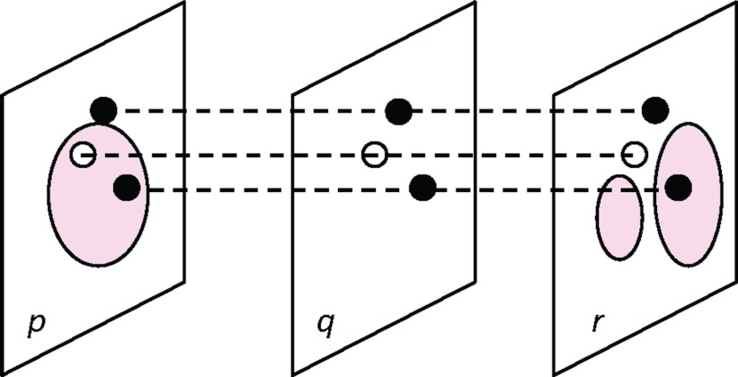
We propose a graph-based interpolation method that reuses the graphs from the already segmented adjacent slices (Figure 3). Let slice q be the slice where the contour is to be interpolated and slices p and r be the two adjacent slices directly above and below. A node is deemed to require re-estimation if its adjacent nodes on slices p and r are assigned to two different classes by our graph cut segmentation. For a node requiring re-estimation, the edge costs are estimated from the sample as regular ones in full segmentation. For a node i on slice q that does not need re-estimation, that is, its adjacent nodes directly above and below are assigned to the same class, we calculate the interpolated edge costs w for node i directly from its adjacent nodes above and below on slice p and r as follows:

$$w_i^q=\frac{d_{pq}}{d_{pq}+d_{qr}}{w}_i^r+\frac{d_{qr}}{d_{pq}+d_{qr}}{w}_i^p,$$ (7)

where d_pq and d_qr are the distances from slice q to slice p, and slice q to slice r, respectively. The interpolated graph then is used to calculate the min s-t cut and obtain the contour.

Figure 3.

Graph-based interpolation. The solid line contours are segmented from our graph cut method on the two slices p and r. On the slice q being interpolated, the nodes in black do not need re-estimation since their adjacent nodes on slice p and r are assigned to the same class. Their edge costs are interpolated as Eq. 7 from slices p and r. The node in white needs re-estimation since its adjacent nodes on slice p and r are assigned to two different classes. A graph min-cut is then applied to the partially interpolated graph on slice q for segmentation.

Evaluation

We refer to our method as semiautomatic adaptive statistical segmentation, or SAASS in our comparison studies.

Phantom

To illustrate the advantage of our proposed probabilistic pair-wise interaction function u_i,j [Eq. 4] for the boundary energy, we synthesize a phantom image containing vertebral structures of the human body using the NCAT phantom software.³¹ We compare SAASS with Boykov's graph cut method^{12, 13} which uses a boundary term defined in Eq. 5 that favors a high contrast boundary. Gaussian noise of 4% standard deviation is added to the image for testing the sensitivity to noise. The result is compared visually.

Clinical cases

For clinical cases, liver segmentation of ten previously treated patients and left kidney segmentation of eight previously treated patients with contrast-enhanced CT images were examined. In our study, the clinical contours of liver and kidney, drawn manually the physicians, served as the ground truth. We set β in Eq. 3 to Eq. 2 in this study for SAASS.

Accuracy

To evaluate the accuracy of our segmentation method in clinical cases, we used two objective evaluations for quantified comparison to other methods. The two objective evaluations are (i) overlay analysis to measure agreement between SAASS-predicted and manually drawn (ground truth) segmentations and (ii) surface distance between SAASS-predicted surface and ground truth.

For the overlay analysis, the terms true positive (TP), true negative (TN), false positive (FP), and false negative (FN) are used to compare the SAASS classification label assignment with that from ground truth. In the context of liver segmentation, for example, TP is the number of predicted liver voxels that are also inside the ground truth segmentation and FP is the number of predicted liver voxels outside ground truth. By definition, sensitivity is TP/(TP+FN), specificity is TN/(TN+FP) and dice similarity coefficient (DSC) is 2×TP/(TP+FN+TP+FP). Evaluation of the accuracy of the boundary from contour delineation is particularly important to radiation treatment planning, as it affects the reliability of the treatment plan in limiting dose to normal tissues. To measure how far the two surfaces are from each other, we use the concept of the two-sided Hausdorff distance.³² For each voxel on the surface of the predicted segmentation, we calculate the distance to the nearest voxel on the surface of the ground truth. We then repeat in reverse order from the ground truth to the predicted surface. Defining the two average distances per surface voxel as d_s→g and d_g→s, respectively, the larger of the two average surface distances, i.e., max{d_s→g, d_g→s}, is chosen as the surface distance metric.

For comparison to other well-known boundary-based semiautomatic methods, we also carried out liver and kidney segmentations using region growing⁴ (RG) developed in-house and state-of-art level set methods in ITK, a well-known medical image processing toolkit supported by NIH. The ITK level set methods are implemented in the MIPAV package³³ from NIH (MIPAV-LS) and in Seg3D package³⁴ from University of Utah (Seg3D-LS). The two packages are widely used standards. RG is an implementation of the classic method. The homogeneity criterion is the mean intensity value inside the region. The threshold for determining a pixel to be included in the region or not is chosen interactively so that the best result is achieved. The MIPAV-LS is a real-time interactive tool. The user moves the mouse around the target organ's boundary and the level set tool updates the contour automatically in real-time as the cursor moves. No parameters need to be specified. Similar to RG, we choose the best segmentation visually when using MIPAV-LS. Seg3D-LS is an iterative level set method that limits the region where the contour evolves using thresholds. We use 600 iterations for liver cases and 160 iterations for kidney cases. The threshold range is mean ±3 standard deviation in image intensity for liver and ±2 standard deviation for kidney. Curvature, propagation and edge weights are default values at 1, 1, and 0, respectively.

We compare our graph-based interpolation method (Sec. 2E) with the mesh-based interpolation method³⁵ developed in-house in our treatment planning system. DSC is used for the comparison with manually drawn contours as the ground truth.

Acceptability

Physicians subjectively evaluated the accuracy of the semiautomatic contours. Three radiation oncology physicians experienced in organ delineation were recruited to review the SAASS contours of ten liver cases. A score is assigned to each contoured slice: 3 = all the three experts agree that no modification is required; 2 = modification is required by one expert; 1 = modification is required by two experts; 0 = modification is required by all three experts. The scores are averaged over the slices for each case.

Interobserver and intraobserver variation

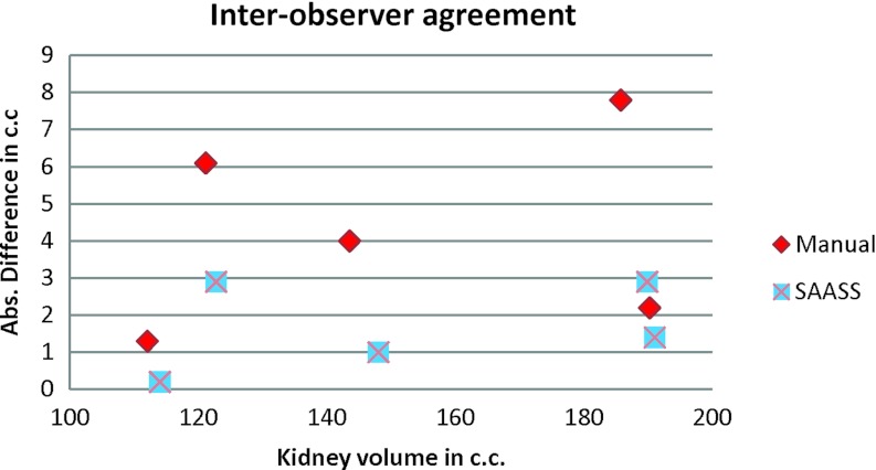
One physician and one resident were recruited to delineate left kidney in five patient cases. In each case, the observer manually drew the contour twice using the paintbrush tool in our in-house treatment planning system and twice using our SAASS tool. The contours from the first round were not visible to the observers when they delineated the contours at the second round. For interobserver variation, only the contours from the first round were used for evaluation.³⁶ The volumes of the left kidneys from the segmentations as well as the difference of the volumes between the segmentations are calculated for plotting the well-known Bland–Altman plots³⁷ to show the agreement.

Time saving

We manually timed the first round of the segmentations in interobserver and intraobserver variation study of five kidney cases for comparing the segmentation time of using manual tool and SAASS. The timer started at the first brush stroke and stopped at the last brush stroke when the observer finished the whole left kidney. The time includes all the GUI interaction. For each case, the mean time per slice is calculated and then the mean times and variations of five cases are averaged for each observer.

RESULTS

Phantom

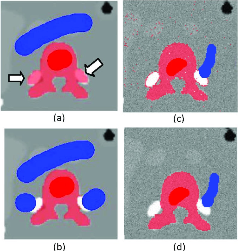
Figure 4 is a visual comparison to demonstrate the problem of gradient-based boundary term that favors high contrast in Boykov's method [Eq. 2] and the advantage of our probability-based boundary term [Eq. 5] in SAASS. The target structure is the vertebra indicated by the red brush strokes while the blue brush strokes indicate the background. Figure 4a shows that Boykov's method (λ = 10, σ = 6) mislabeled the nearby rib structures due to their higher contrast. This mislabeling necessitated additional manual corrections [Fig. 4b]. The addition of Gaussian noise to the phantom image shows that, even with heavily weighted regional terms (λ = 0.1), i.e., likelihood of the pixel intensity to belong to target and nontarget regions, Boykov's method cannot achieve a clean segmentation (piece-wise continuity) due to noisy pixels [Fig. 4c]. In contrast, the SAASS requires fewer brush strokes to obtain correct and clean segmentation results [Fig. 4d].

Figure 4.

Segmentation results from the phantom image. (a) On noise-free images, Boykov's boundary term favoring high contrast [Eq. 5] is prone to leakage if a high contrast boundary is present in nearby tissue (arrow). (b) Additional brush strokes are needed to exclude neighboring tissue. (c) On an image with 4% Gaussian noise, using Boykov's boundary term and strongly weighted regional term results in an irregular boundary and pixels within the segmentation are excluded. (d) In contrast, our method SAASS requires fewer brush strokes and preserves piece-wise continuity.

Clinical CT images

Instead of using a training set, we trained our method individually with locally obtained samples (Sec. 2D) in each case. For each study, a single slice in the middle of the 3D stack is first segmented manually for boundary training. The boundary samples from this training slice are used to estimate the statistical boundary interaction potential for the remaining slices without retraining. The single slice boundary samples provided sufficient accuracy in our study while saving the time that would have been needed for rebuilding a 2D ASH histogram on every slice. Regional statistics are obtained adaptively from the seed voxels under the user specified brush strokes.

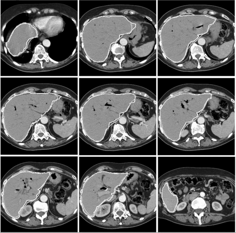
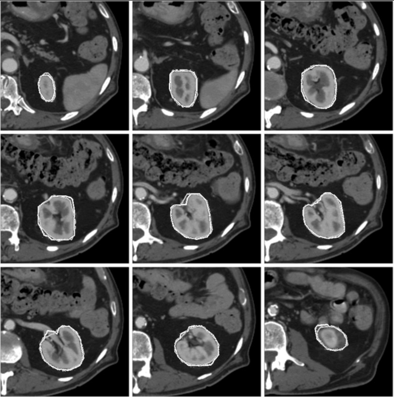
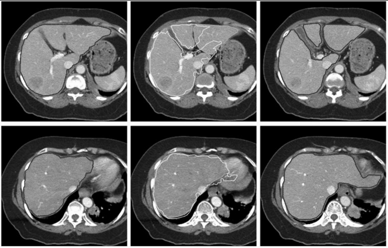
Figures56 show the contours from SAASS and the contours drawn by physician for a liver case and a kidney case, respectively. SAASS contours closely matched the physician contours. The second image in the top row of the liver case shows some discrepancy in the upper right region, where the boundary contrast is low. SAASS handled the intensity inhomogeneity of the kidney well due to the use of regional statistics in our energy function.

Figure 5.

Liver segmentation of a patient. Typical image slices from superior to inferior are shown. Physician-drawn contours in dark gray and SAASS contours are in light gray.

Figure 6.

Kidney segmentation of a patient. Typical image slices from superior to inferior are shown. Physician-drawn contours in dark gray and SAASS contours are in light gray.

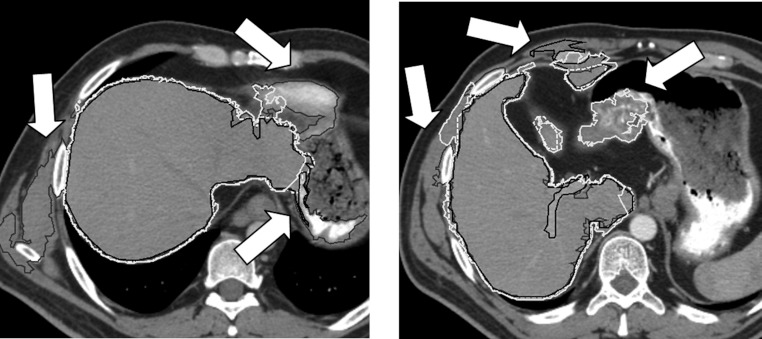
Figure 7 shows CT slices where SAASS performs well on the slices where RG, MIPAV-LS, and Seg3D-LS suffer from leakage into surrounding tissue, due to the low-contrast boundary between target organ and surrounding tissue or the relative high contrast of the surrounding tissues. Both the probabilistic boundary terms and the user guided approach through interactive paint brushes contribute to the superior performance of SAASS.

Figure 7.

Comparison of liver segmentations: SAASS (dashed white), RG (black), MIPAV-LS (dark gray), and Seg3D-LS (light gray). RG, MIPAV-LS, and Seg3D-LS segmentations show leakage (arrows) since they are sensitive to low-contrast boundary and surrounding high contrast tissues.

Overlay analysis

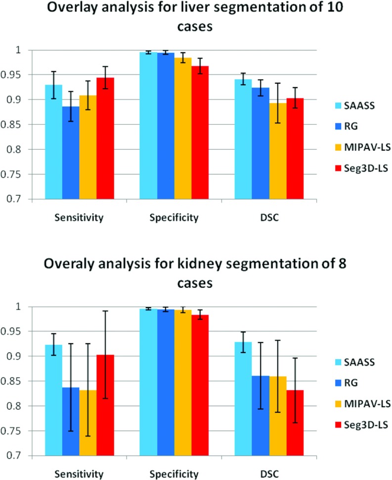
Figure 8 shows comparison of the sensitivity, specificity, and DSC between the four methods in liver and kidney segmentations. SAASS has the best DSC in both liver (94 ± 3%) and kidney (93 ± 2%) among these methods.

Figure 8.

Overlay analysis for liver and kidney segmentation. SAASS has the best DSC and smallest variation among the four methods compared.

Surface distance analysis

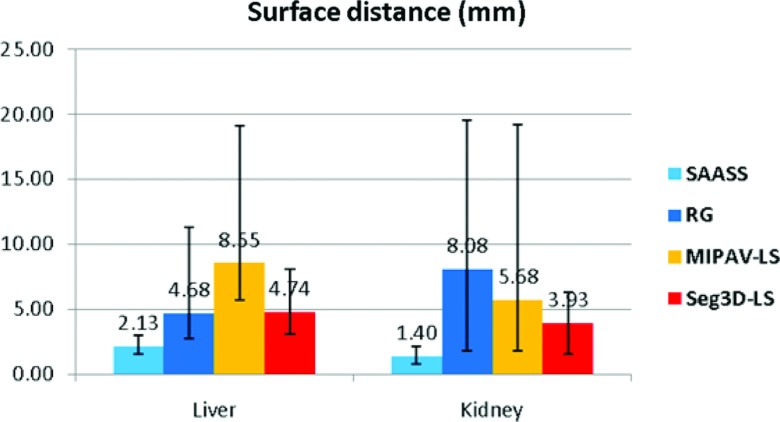
Figure 9 summarizes the mean Hausdorff surface distances (over boundary voxels) from SAASS as well as segmentation from RG, MIPAV-LS, and Seg3D-LS methods in liver and kidney. The mean±one-standard-deviation Hausdorff distances for SAASS are 2.13 ± 0.49 mm over the ten liver cases and 1.40 ± 0.39 mm over the eight kidney cases, which are smaller than the other methods.

Figure 9.

Mean Hausdorff distance comparison in ten liver cases and eight kidney cases. Error bars show the minimum and maximum distances over the cases.

Subjective measure-acceptability score

Table 1 shows the expert evaluation scores for ten liver cases. Among a total of 639 slices, 83% required no modification, 11% required modifications by any single physician, 5% required modifications mutually agreed by any two physicians and 1% required modification agreed by all three physicians.

Table 1.

Scores of ten liver cases evaluated by three physicians. See text for details of the scoring rules.

	Liver case (number of slices)
Score	1(63)	2(71)	3(53)	4(62)	5(76)	6(68)	7(66)	8(45)	9(72)	10(63)
3	55	58	43	42	65	54	57	38	62	56
2	2	10	9	9	9	6	6	4	7	7
1	6	2	1	9	1	7	3	1	1	0
0	0	1	0	2	1	1	0	2	2	0
Average	2.78	2.76	2.79	2.47	2.82	2.66	2.82	2.73	2.79	2.89

Graph-based interpolation

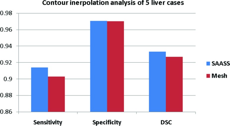
Figure 10 compares the sensitivity, specificity, and DSC between our graph-based interpolated method (Sec. 2E) in SAASS and traditional surface mesh-based interpolation method in five liver cases. Only the slices where the liver topology changed from two lobes to three lobes are used for comparison. Our method has higher DSC (93.3 ± 3.8%) than mesh-based method (92.7 ± 3.9%). Figure 11 shows the slices where SAASS shows its advantage over meshed-based methods. The top row of images shows a change in liver topology: from one lobe in the left image to three lobes in the middle and right images. Our graph-based interpolation method avoids the branching problem that is difficult to solve using surface tiling interpolation (top middle image). Even without a change of topology, our method still shows improved performance over mesh-based methods which do not use image information (bottom middle image). Our method uses regional information from the previously constructed graphs of the adjacent slices as well as local regional information re-estimated in the transitional area where the nodes of adjacent slices are segmented into different tissue classes.

Figure 10.

Sensitivity, specificity, and DSC measures comparison between SAASS graph-based interpolation and mesh-based interpolation. Mean of the measures in five liver cases are shown.

Figure 11.

(Top row) Image slices where liver topology changes. The light gray contours in the middle slice are interpolated from the dark gray contours in the adjacent slices on the left and right based on surface tiling method, but suffer from topological change. The pale gray contours are result of our graph-based interpolation method (Sec. 2E). (Bottom row) Even without topological change, our method still shows improved performance over surface tiling (middle), due the utilization of image information.

Interobserver and Intraobserver analysis

Figure 12 shows a Bland–Altman plot of interobserver agreement in five kidney cases. The x axis is the volume of kidney and y axis is the absolute difference in volume. SAASS has smaller variation compared to the manual method. Figure 13 shows the Bland–Altman plots of intraobserver agreement for Observer 1 and Observer 2. In both observers, SAASS has better agreement compared to the manual method.

Figure 12.

Bland–Altman plot of interobserver agreement in five kidney cases. Absolute value of the difference is used in y axis. SAASS shows better repeatability and the difference is irrelevant to the size of volumes.

Figure 13.

Bland–Altman plots of intraobserver agreement for Observer 1 and Observer 2. In both observers, SAASS has better agreement compared to the manual method.

Time saving

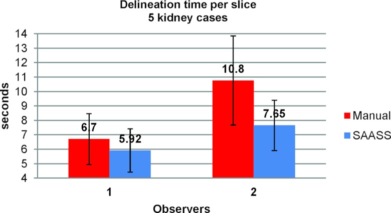
Figure 14 shows mean time per slice for segmentations of five kidney cases from the two observers. Compared to manual segmentation, on average, SAASS performs faster, 12% and 29% for Observer 1 and Observer 2, respectively, than the manual delineation. Based on our recorded video, one observer tended not to review the manual segments once they were done, but did spend more time reviewing the SAASS segments.

Figure 14.

Comparison of performance of the manual method and SAASS. Mean time per slice for segmentations of five kidney cases is calculated from the two observers. The error bars show one standard deviation.

DISCUSSION AND CONCLUSIONS

Manual delineation of organs and other structures in CT is one of the most time consuming processes performed in radiation treatment planning. It becomes more problematic with greater amounts of image data produced by recent, as well as future, advanced imaging devices. Researchers have investigated various automatic and semiautomatic segmentation methods for radiation treatment planning. The clinical usability of automatic methods, however, is commonly limited by speed due to the iterative convergence approach, especially for a large organ; by robustness due to poor model initialization, weak image features and large variation in organs; or restricted due to application-, site-, and structure-specific heuristics techniques that need special parameter tuning. The goal of our work is to develop a method that avoids these limitations so that the segmentation tool is easy to use with high level of automation while maintaining human experts’ oversight.

We have proposed a purely statistical semiautomatic 2.5 D medical image segmentation method that obtains a MAP estimation of image segmentation in a CRF framework via a noniterative and rapid graph cut optimization. Our method learns statistical boundary and regional information from a few experts’ brush strokes to achieve accuracy similar to manual segmentation but with less fatigue and time.

Results with clinical images indicate that the boundary statistics from a single slice can be reused for the entire image stack without retraining to achieve high accuracy. It should be noted that the boundary training can also be adaptive, that is, the boundary samples are accumulated from previously segmented slices. This, however, needs further investigation on the trade-off between accuracy improvement and the time expense on updating the histogram. Results in liver also show that our method is less prone to boundary leakage than region growing and level set methods. This is due to the use of both probabilistic regional and boundary terms in our energy function derived from CRF. Consequently, because of this statistical framework, our method requires less brush strokes than previous graph cut methods and manual methods thus the time required for manual interaction is reduced. In interobserver and intraobserver analysis, our method shows better agreement than the manual method thus provides more consistent contour delineation while the delineation time is considerably reduced. This is extremely important when the target anatomy volume is large and fast and accurate segmentation is highly desired.

In the evaluation of clinical images, we have used physician-drawn contours of liver and kidney as a ground truth. Defining a ground truth in a medical context, however, is not trivial. One of our referenced papers³⁶ in the application of liver transplants establishes true ground truth volume by measuring the volume of surgically removed livers. Human delineations of medical images are not a true gold standard but are the most objective solution.¹⁸ We refer to Bouix et al.³⁸ for a comprehensive discussion on ground truth in segmentations.

As we mentioned in Sec. 2, for some organs the intensity distributions of target organ and nearby nontarget tissue are nearly identical and the boundary between them is of low contrast, such as the liver left lobe and the apex of the heart shown in Fig. 15a. For such cases, all segmentation algorithms that are based on intensities, including ours, will have leakage if there is no evidence in the intensity image for a change from one tissue to the next. The algorithm classified part of the heart as liver, shown in Fig. 15b. In such cases extra information is needed to correctly separate the tissues. Our algorithm naturally integrates this information from expert intervention. The boundary is corrected with an additional brush stroke as shown in Fig. 15c. The CRF framework, however, allows the inclusion of an organ-specific probabilistic atlas,^{39, 40} which will provide positional probability estimation that works as a shape prior in addition to our probabilistic regional and boundary terms for better control of the leakage.

Figure 15.

An example to demonstrate leakage. (a) The image shows blurred boundary between the liver left lobe and the apex of the heart. (b) Leakage of the initial segmentation due to blurred boundary. (c) An additional brush stroke to remove the leakage. The ground truth contour is shown.

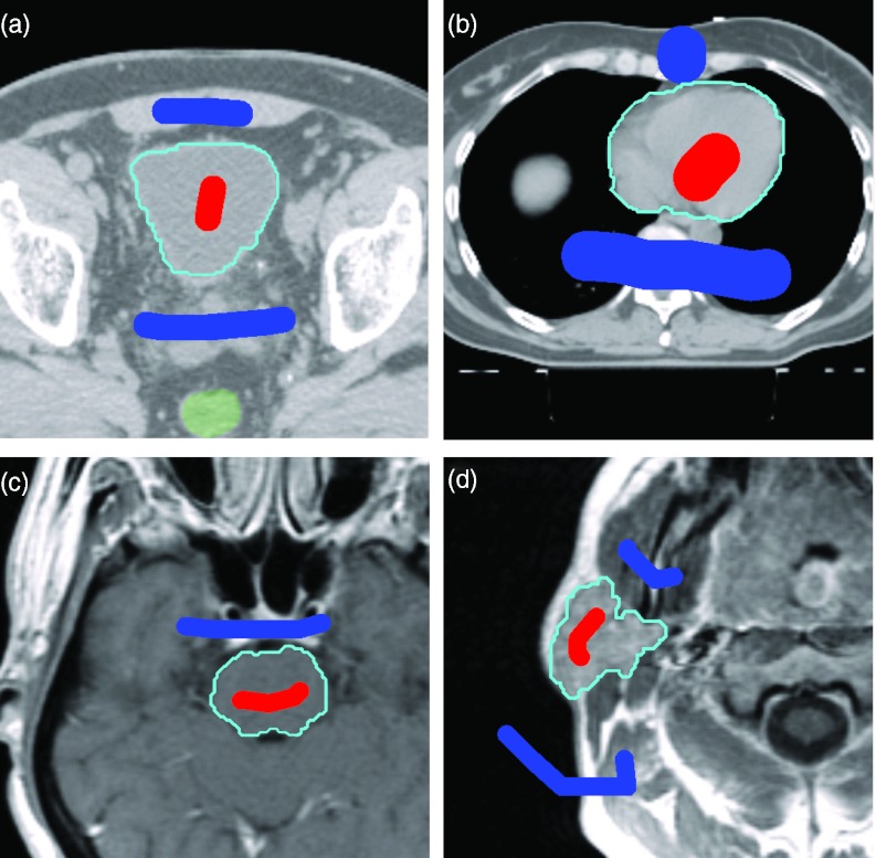
Our framework using CRF is extremely flexible. It is not organ-specific or modality-specific. Preliminary work indicates that the technique is also applicable to MR but an extensive evaluation of other modalities is outside the scope of this paper. Figure 16 shows examples of bladder and heart segmentations in CT, and brain-stem and parotid segmentation in MR images.

Figure 16.

Examples of segmentation on other organs and other modalities: (a) bladder and (b) heart in CT; (c) brainstem and (d) parotid in MR images. We note that MR inhomogeneity in pixel intensity should be corrected prior to intensity-based segmentation methods.

Our current investigations are to extend this method to 3D and explore more sophisticated image features, such as the probabilistic atlas, within the same CRF framework that defines the energy function and uses the graph cut optimization scheme.

References

- Fox J. L., Rosenzweig K. E., Rengan R., O’Meara W., Yorke E., Erdi Y., Nehmeh S., and Leibel S. A., “Does the registration of PET and planning CT images decrease inter-and intra-observer variation in delineating tumor volumes for non-small-cell lung cancer (NSCLC)?,” Int. J. Radiat. Oncol., Biol., Phys. 62, 70–75 (2005). 10.1016/j.ijrobp.2004.09.020 [DOI] [PubMed] [Google Scholar]
- Bae K. T., Giger M. I., Chen C. T., and Kahn C. E., “Automatic segmentation of liver structure in CT images,” Med. Phys. 20, 71–78 (1993). 10.1118/1.597064 [DOI] [PubMed] [Google Scholar]
- Gao L., Heath D. G., Kuszyk B. S., and Fishman E. K., “Automatic liver segmentation technique for three-dimensional visualization of CT data,” Radiology 201, 359–364 (1996). [DOI] [PubMed] [Google Scholar]
- Adams R. and Bischof L., “Seeded region growing,” IEEE Trans. Pattern Anal. Mach. Intell. 16(6), 641–647 (1994). 10.1109/34.295913 [DOI] [Google Scholar]
- Pohle R. and Toennies K. D., “Segmentation of medical images using adaptive region growing,” Proc. SPIE Med. Imaging: Image Process. 4322, 1337–1346 (2001). 10.1117/12.431013 [DOI] [Google Scholar]
- Ruskó L., Bekes G., Németh G., and Fidrich M., “Fully automatic liver segmentation for contrast-enhanced CT images,” in Proceedings of MICCAI Workshop on 3-D Segmentation in the Clinic: A Grand Challenge (2007), pp. 143–150.
- Liu F., Zhao B., Kijewski P., Wang L., and Schwartz L., “Liver segmentation for CT images using GVF snake,” Med. Phys. 32(12), 3699–3706 (2005). 10.1118/1.2132573 [DOI] [PubMed] [Google Scholar]
- Lim S. J., Jeong Y.-Y., and Ho Y.-S., “Segmentation of the liver using the deformable contour method on CT images,” Advances in Multimedia Information Processing - PCM 2005: Lect. Notes Comput. Sci. 3767, 570–581 (2005). [Google Scholar]
- Suzuki K., Kohlbrenner R., Epstein M. L., Obajuluwa A. M., Xu J., and Hori M., “Computer-aided measurement of liver volumes in CT by means of geodesic active contour segmentation coupled with level-set algorithms,” Med. Phys. 37(5), 2159–2166 (2010). 10.1118/1.3395579 [DOI] [PMC free article] [PubMed] [Google Scholar]
- Barrett W. A. and Mortensen E. N., “Interactive live-wire boundary extraction,” Med. Image Anal. 1, 331–341 (1997). 10.1016/S1361-8415(97)85005-0 [DOI] [PubMed] [Google Scholar]
- Schenk A., Prause G., and Peitgen H., “Efficient semiautomatic segmentation of 3D objects in medical images,” in Proceedings of Medical Image Computing and Computer-assisted Intervention (MICCAI) (Springer, Berlin/Heidelberg, 2000), pp. 186–195.
- Boykov Y. and Jolly M. P., “Interactive graph cuts for optimal boundary & region segmentation of objects in N-D images,” Proc. Int. Conf. Comput. Vis. I, 105–112 (2001). 10.1109/ICCV.2001.937505 [DOI] [Google Scholar]
- Boykov Y. and Funka-Lea G., “Graph cuts and efficient N-D image segmentation,” Int. J. Comput. Vis. 70, 109–131 (2006). 10.1007/s11263-006-7934-5 [DOI] [Google Scholar]
- Burnett S. S. C., Starkschall G., Stevens C. W., and Liao Z., “A deformable-model approach to semi-automatic segmentation of CT images demonstrated by application to the spinal canal,” Med. Phys. 31(2), 251–263 (2004). 10.1118/1.1634483 [DOI] [PubMed] [Google Scholar]
- Pekar V., McNutt T. R., and Kaus M. R., “Automated model-based organ delineation for radiotherapy planning in prostatic region,” Intl. J. of Radiat. Oncol., Biol., Phys. 60(3), 973–980 (2004). 10.1016/j.ijrobp.2004.06.004 [DOI] [PubMed] [Google Scholar]
- Rao M., Stough J., Chi Y.-Y., Muller K., Tracton G., Pizer S. M., and Chaney E. L., “Comparison of human and automatic segmentations of kidneys from CT images,” Int. J. Radiat. Oncol., Biol., Phys. 61(3), 954–960 (2005). 10.1016/j.ijrobp.2004.11.014 [DOI] [PubMed] [Google Scholar]
- Pasquier D., Lacornerie T., Vermandel M., Rousseau J., Lartigau E., and Betrouni N., “Automatic segmentation of pelvic structures from magnetic resonance images for prostate cancer radiotherapy,” Int. J. Radiat. Oncol., Biol., Phys. 68(2), 592–600 (2007). 10.1016/j.ijrobp.2007.02.005 [DOI] [PubMed] [Google Scholar]
- Heimann T., van Ginneken B., Styner M., Arzhaeva Y., Aurich V., Bauer C., Beck A., Becker C., Beichel R., Bekes G., Bello F., Binnig G., Bischof H., Bornik A., Cashman P. M. M., Chi Y., Cordova A., Dawant B. M., Fidrich M., Furst J., Furukawa D., Grenacher L., Hornegger J., Kainmueller D., Kitney R. I., Kobatake H., Lamecker H., Lange T., Lee J., Lennon B., Li R., Li S., Meinzer H.-P., Nemeth G., Raicu D. S., Rau A.-M., van Rikxoort E. M., Rousson M., Rusko L., Saddi K. A., Schmidt G., Seghers D., Shimizu A., Slagmolen P., Sorantin E., Soza G., Susomboon R., Waite J. M., Wimmer A., and Wolf I., “Comparison and evaluation of methods for liver segmentation from CT datasets,” IEEE Trans. Med. Imaging 28(8), 1251–1265 (2009). 10.1109/TMI.2009.2013851 [DOI] [PubMed] [Google Scholar]
- Lafferty J., McCallum A., and Pereira A. F., “Conditional random fields: Probabilistic models for segmenting and labeling sequence data,” in Proceedings 18th International Conference on Machine Learning (Morgan Kaufmann, Burlington, MA, 2001), pp. 282–289.
- Wallach H. M., “Conditional random fields: An introduction,” Technical Report No. MS-CIS-04-21 (University of Pennsylvania, 2004).
- Kumar S. and Hebert M., “Discriminative random fields: A discriminative framework for contextual interaction in classification,” Proc. Int. Conf. Comput. Vis. 2, 1150–1157 (2003). 10.1109/ICCV.2003.1238478 [DOI] [Google Scholar]
- Greig D., Porteous B., and Seheult A., “Exact maximum a posteriori estimation for binary images,” J. R. Stat. Soc. Ser. B (Methodol.) 51, 271–279 (1989). [Google Scholar]
- Kass M., Witkin A., and Terzopoulos D., “Snakes: Active contour models,”Int. J. Comput. Vis. 1, 321–331 (1988). 10.1007/BF00133570 [DOI] [Google Scholar]
- Xu C. and Prince J. L., “Gradient vector flow: A new external force for snakes” in Proceedings of the Conference on Computer Vision and Pattern Recognition (CVPR), 1997 (Computer Society Press, Los Alamitos, 1997), pp. 66–71.
- Sethian J. A., Level Set Methods and Fast Marching Methods (Cambridge University Press, Cambridge, England, 1999). [Google Scholar]
- Malladi R., Sethian J., and Vemuri B. C., “Shape modeling with front propagation: A level set approach,” IEEE Trans. Pattern Anal. Mach. Intell. 17(2), 158–175 (1995). 10.1109/34.368173 [DOI] [Google Scholar]
- Wu Z. and Leahy R., “An optimal graph theoretic Approach to data clustering: Theory and its application to image segmentation,” IEEE Trans. Pattern Anal. Mach. Intell. 15(13), 1101–1113 (1993). 10.1109/34.244673 [DOI] [Google Scholar]
- Kolmogorov V. and Zabih R., “What energy functions can be minimized via graph cuts?,” IEEE Trans. Pattern Anal. Mach. Intell. 26(2), 147–59 (2004). 10.1109/TPAMI.2004.1262177 [DOI] [PubMed] [Google Scholar]
- Hu Y.-C., Grossberg M. D., and Mageras G. S., “Semi-automatic medical image segmentation with adaptive local statistics in conditional random fields framework,” Proc. IEEE Conf. Eng. Med. Biol. Soc. 2008, 3099–102. 10.1109/IEMBS.2008.4649859 [DOI] [PMC free article] [PubMed] [Google Scholar]
- Scott D., “Average shifted histograms: Effective nonparametric density estimators in several dimensions,” Ann. Stat. 13, 1024–1040 (1985). 10.1214/aos/1176349654 [DOI] [Google Scholar]
- Garrity J. M., Segars W. P., Knisley S. B., and Tsui B. M. W., “Development of a dynamic model for the lung lobes and airway tree in the NCAT phantom,” IEEE Trans. Nucl. Sci. 50(3), 378–383 (2003). 10.1109/TNS.2003.812445 [DOI] [Google Scholar]
- Cignoni P., Rocchini C., and Scopigno R., “Metro: Measuring error on simplified surfaces,” Comput. Graph. Forum 17(2), 167–174 (1998). 10.1111/1467-8659.00236 [DOI] [Google Scholar]
- McAuliffe M., Lalonde F., McGarry D., Gandler W., Csaky K., and Trus B., “Medical image processing, analysis and visualization in clinical research,” in Proceedings of the 14th IEEE Symposium on Computer-Based Medical Systems (CBMS) (2001), pp. 381–386. 10.1109/CBMS.2001.941749 [DOI]
- Institute, S. C. a. I. “‘Seg3D’ volumetric image segmentation and visualization. scientific computing and imaging institute (SCI),” from http://www.seg3d.org.
- Fuchs A. H., Kedem A. Z. M., and Uselton A. S. P., “Optimal surface reconstruction from planar contours,” J. Commun. ACM 20(10), 693–702 (1977). 10.1145/359842.359846 [DOI] [Google Scholar]
- Hermoye L., Laamari-Azjal I., Cao Z., Lerut J., Dawant B. M., and Van Beers B. E., “Liver segmentation in living liver transplant donors: Comparison of semiautomatic and manual methods,” Radiology 234(1), 171–178 (2005). 10.1148/radiol.2341031801 [DOI] [PubMed] [Google Scholar]
- Altman D. G. and Bland J. M., “Measurement in medicine: The analysis of method comparison studies,” J. R. Stat. Soc. Ser. B (Methodol.) 32(3), 307–317 (1983). 10.2307/2987937 [DOI] [Google Scholar]
- Bouix S., Martin-Fernandez M., Ungar L., Nakamura M., Koo M.-S., McCarley R. W., and Shentona M. E., “On evaluating brain tissue classifiers without a ground truth,” NeuroImage 36, 1207–1224 (2007). 10.1016/j.neuroimage.2007.04.031 [DOI] [PMC free article] [PubMed] [Google Scholar]
- Park H., Bland P., and Meyer C., “Construction of an abdominal probabilistic atlas and its application in segmentation,” IEEE Trans. Med. Imaging 22, 483–492 (2003). 10.1109/TMI.2003.809139 [DOI] [PubMed] [Google Scholar]
- Linguraru M. G., Sandberg J. A., Li Z., Shah F., and Summers R. M., “Automated segmentation and quantification of liver and spleen from CT images using normalized probabilistic atlases and enhancement estimation,” Med. Phys. 37(2), 771–783 (2010). 10.1118/1.3284530 [DOI] [PMC free article] [PubMed] [Google Scholar]