Mapping the Tonotopic Organization in Human Auditory Cortex with Minimally Salient Acoustic Stimulation

Abstract

Despite numerous neuroimaging studies, the tonotopic organization in human auditory cortex is not yet unambiguously established. In this functional magnetic resonance imaging study, 20 subjects were presented with low-level task-irrelevant tones to avoid spread of cortical activation. Data-driven analyses were employed to obtain robust tonotopic maps. Two high-frequency endpoints were situated on the caudal and rostral banks of medial Heschl's gyrus, while low-frequency activation peaked on its lateral crest. Based on cortical parcellations, these 2 tonotopic progressions coincide with the primary auditory field (A1) in lateral koniocortex (Kl) and the rostral field (R) in medial koniocortex (Km), which together constitute a core region. Another gradient was found on the planum temporale. Our results show the bilateral existence of 3 tonotopic gradients in angulated orientations, which contrasts with colinear configurations that were suggested before. We argue that our results corroborate and elucidate the apparently contradictory findings in literature.

Introduction

Tonotopy is a key organizational feature of the vertebrate auditory system. Also referred to as cochleotopy, it arises in the cochlea of the inner ear, which acts as a bank of parallel filters that are sharply tuned to neighboring frequencies (von Bekesy 1949). Because this organization pervades all levels of the central auditory system—including the auditory nerve, subcortical nuclei, and auditory cortex—it forms one of the most characteristic functional principles to guide our understanding of auditory processing. In that sense, it is comparable to the role of retinotopy in the visual system and somatotopy in the somatosensory and motor systems. However, in sharp contrast with these other topographic cortical mappings, the tonotopic layout of the human auditory cortex remains relatively poorly understood.

Electrophysiologic recordings in numerous animal species, including birds (Cohen and Knudsen 1996; Capsius and Leppelsack 1999; Terleph et al. 2006), rodents (Merzenich et al. 1976; Hellweg et al. 1977; McMullen and Glaser 1982; Kelly et al. 1986; Stiebler et al. 1997), primates (Luethke et al. 1989; Morel and Kaas 1992; Kusmierek and Rauschecker 2009; Scott et al. 2011), and other mammals (Suga and Jen 1976; Tunturi and Barrett 1977; Reale and Imig 1980), have repeatedly shown the existence of multiple cortical fields that display a tonotopic organization. Often, at least 2 pronounced frequency gradients are observable in primary auditory cortex that are more or less colinear but oppositely directed and abutting at their low-frequency endpoint. This results in a distinctive “high-to-low-to-high” distribution of characteristic frequencies. Because in humans such invasive measurements can be carried out in exceptional circumstances only, direct recordings of characteristic frequency as a function of location in human auditory cortex are sparse (Howard et al. 1996). More recently, animal studies also started to use noninvasive methods, and the observable extensive tonotopic patterns are now regularly relied upon to reveal a multitude of functional fields in auditory cortex (Petkov et al. 2006, 2009; Tanji et al. 2010). At the same time, various specializations and differentiations that are unique to humans, both in function (e.g., language) and in structure (e.g., Heschl's gyrus, HG), may have given rise to a different tonotopic layout as compared with other mammals. This complicates the translation of results from animals to humans.

Many studies have attempted to map the tonotopic organization in healthy human subjects. Electroencephalographic (EEG) and magnetoencephalographic (MEG) data allow the effective location of current dipoles to be reconstructed, typically one for each hemisphere. A number of studies reported that the dipole's depth below the scalp and its coordinate along the rostrocaudal axis increased with stimulus frequency, and its orientation varied due to gyral morphology (Romani et al. 1982; Pantev et al. 1988; Kuriki and Murase 1989; Cansino et al. 1994; Pantev et al. 1994; Huotilainen et al. 1995; Verkindt et al. 1995; Gabriel et al. 2004; Weisz, Wienbruch, et al. 2004; Wienbruch et al. 2006; Ozaki and Hashimoto 2007). These findings confirm that human auditory cortex is organized tonotopically, with an effective low-to-high-frequency gradient extending in the (antero)lateral-to-(postero)medial direction along HG. However, in spite that at least 2 studies distinguished multiple tonotopic gradients in one hemisphere simultaneously (Pantev et al. 1995; Weisz, Keil, et al. 2004), the coarse spatial resolution and limited number of reconstructable dipoles in EEG/MEG presently restricts the ability to map cortical frequency representations in closer detail.

Alternative neuroimaging modalities, like positron emission topography (PET) and functional magnetic resonance imaging (fMRI), offer more precise spatial resolution and the ability to sample large numbers of cortical sites simultaneously. Early studies determined the effective location of activation in each hemisphere (e.g., the center of mass of an activation cluster or the location of its peak activation) in response to as little as 2 different tone frequencies but still confirmed that the higher frequency was represented more (postero)medially along HG than the lower frequency (Lauter et al. 1985; Wessinger et al. 1997; Bilecen et al. 1998; Lockwood et al. 1999). Later, more frequencies were included in an attempt to show that the tonotopic progression in primary auditory cortex was gradual (Le et al. 2001; Petkov et al. 2004; Scarff et al. 2004; Yetkin et al. 2004; Langers et al. 2007), although at least one report considered the possibility that functional fields with discrete differences in their frequency preferences could also explain the observed data (Schönwiesner et al. 2002).

Other authors have attempted to distinguish multiple tonotopic gradients per hemisphere. For example, 8 consistently occurring response foci to either low- or high-frequency stimuli were identified (Talavage et al. 2000). Later, these were judged to be pairwise connected by 6 tonotopic gradients on the basis of waves of activation that traveled across the cortex in response to slow frequency sweeps (Talavage et al. 2004). Multiple low-to-high-frequency gradients were oriented around the lateral-to-medial direction, but results also included an oppositely oriented gradient on the lateral side, for instance. In the same period, a reversed tonotopic organization in lateral temporal cortex was reported (Yang et al. 2000) that was attributed to the existence of a second gradient along lateral HG (Engelien et al. 2002). Through the use of a high-field-strength scanner, appealing evidence soon appeared for the simultaneous existence of 2 mirror-symmetric tonotopic maps in adjacent subdivisions of primary auditory cortex (Formisano et al. 2003). These maps were oppositely directed and extended more or less colinearly along the axis of HG, touching at their low-frequency endpoints. Comparable maps were later observed at lower field strengths (Seifritz et al. 2006; Upadhyay et al. 2007; Woods et al. 2009; Hertz and Amedi 2010). A recent study showed up to 6 gradients extending as far as the superior temporal sulcus and middle temporal gyrus (Striem-Amit et al. 2011). These included the typical mirror-symmetric organization in core auditory cortex, and an additional similar organization in belt and parabelt areas. Taken together, these findings support a picture that is related to that in primates and other mammals (for a meta analysis, see Woods and Alain 2009).

In a recent study (Humphries et al. 2010), a zone on the lateral aspect of HG was found to respond preferentially to lower frequencies, whereas zones posterior and anterior to HG were more sensitive to higher frequencies. An alternative tonotopic organization was proposed in which the gradients are directed obliquely and roughly perpendicular to HG rather than parallel along HG. A third smaller gradient was observed in the lateral planum temporale (PT). The authors claimed that their results still suggest close homologies between the tonotopic organization of human and nonhuman primate auditory cortex but in a different spatial orientation than previously assumed.

In conclusion, most studies in humans agree on the existence of a dominant gradient in which low frequencies are represented laterally and high frequencies are represented medially around HG. Nevertheless, a more detailed tonotopic organization in human auditory cortex is not unambiguously established yet. So why has it proved so problematic to map frequency distributions in human auditory cortex with sufficient precision to identify individual tonotopic gradients?

Various factors complicate the interpretation of functional outcomes. Apart from tonotopic frequency maps, auditory cortex also features representations of other acoustic parameters like stimulus bandwidth, sweep direction, or lateralization (Woods et al. 2010). Furthermore, the morphology of superior temporal cortex is complex and difficult to oversee. At the same time, the functional architecture of the auditory cortex does not relate one-on-one to structural landmarks and shows considerable intersubject variability (Rademacher et al. 2001). Various authors have advocated the mapping of tonotopic gradients in individual subjects, arguing that the functional organization is too variable to be successfully pooled. However, due to the limited amount of data that is usually available from single subjects, this results in worse signal-to-noise characteristics. Also, it renders one vulnerable to individual anomalies that are not representative for the population as a whole.

On top of the complexity of the functional organization in the brain, fundamental methodological limitations play a role. Tonotopic gradients are defined as an orderly progression of neuronal characteristic frequencies across the cortical surface. In turn, the characteristic frequency is defined as that frequency at which a neuron exhibits its lowest response threshold. However, most noninvasive neuroimaging methods tend to have insufficient sensitivity to measure reliable responses near threshold. For that reason, stimuli are typically presented at high intensity levels, where neurons are known to respond to a broad range of frequencies (Recanzone et al. 2000). Moreover, previous studies mostly employed either an auditory task or passive listening to salient sound stimuli to obtain sufficiently high evoked response amplitudes. It is known that neuronal response properties can rapidly be modulated by top-down attentional mechanisms (Bidet-Caulet et al. 2007; Woods et al. 2009; Ahveninen et al. 2011; Paltoglou et al. 2011). By directing attention to task-relevant sound stimuli, tonotopically organized frequency preferences may have been influenced by the experimental paradigm. Typically, task-relevant frequencies tend to be facilitated and become overrepresented in auditory cortex (Fritz et al. 2003). Therefore, stimulus loudness as well as task relevance results in spread of activation, which may distort and possibly obscure any existing tonotopic gradients (Tanji et al. 2010).

In an effort to overcome some of the mentioned difficulties, in the current study, we employed task-irrelevant unattended low-level stimuli to avoid excessive spread of sound-evoked activation. High-resolution fMRI images were acquired to detect responses to tone stimuli that were presented in the absence of acoustic scanner noise and that spanned a 5-octave frequency range. A relatively large group of 20 subjects was included. Using an analysis approach that was strongly data driven, we combined responses across both subjects and stimuli to obtain robust tonotopic maps at the group level.

Materials and Methods

Subjects

Twenty healthy subjects (gender: 4 males, 16 females; age: mean 33 years, range 21–60 years; handedness: 17 right, 3 left) were invited to participate in this fMRI study on the basis of written informed consent, in approved accordance with the requirements of the institution's medical ethical committee. They reported no history of auditory, neurological, or psychiatric disorders. Standard audiometry was performed to determine hearing thresholds for both ears at frequencies from 250 Hz to 8 kHz.

Data Acquisition

Subjects were placed supinely in the bore of a 3.0-T MR system (Philips Intera, Best, the Netherlands), which was equipped with an 8-channel phased-array (SENSE) transmit/receive head coil. The functional imaging session included three 8-min runs, each consisting of a dynamic series of 40 identical high-resolution T₂*-sensitive gradient-echo echo-planar imaging (EPI) volume acquisitions (repetition time 12.0 s; acquisition time 2.0 s; echo time 22 ms; flip angle 90°; matrix 128 × 128 × 40; resolution 1.5 × 1.5 × 1.5 mm³; interleaved slice order, no slice gap). The acquisition volume was positioned in an oblique axial orientation, tilted forward parallel to the Sylvian fissure, and approximately centered on the superior temporal sulci. Additional preparation scans were used to achieve stable image contrast and to trigger the start of stimulus delivery, but these were not included into the analysis. The scanner coolant pump and fan were turned off during imaging to diminish ambient noise levels. The paradigm is illustrated in Figure 1.

Figure 1.

For each subject, 3 runs were performed that consisted of 40 consecutive trials of a visual/emotional task. Each trial comprised 5 s during which a fixation cross was shown, 5 s during which a picture was displayed, and an additional 2 s during which subjects could respond and indicate their judgment of the picture's emotional valence (positive/neutral/negative) with 1 of 3 button options. Sparse fMRI acquisitions took place during the last 2-s interval only; in the interspersed 10-s periods of scanner inactivity, tone sequences were presented. Within a trial, the fundamental frequency (¼, ½, 1, 2, 4, or 8 kHz) and loudness (soft or loud, differing by 20 dB) of the tones remained the same, but these conditions (plus a silent condition) were varied across trials in a random fashion unrelated to the task.

Task

During each imaging run, subjects performed an engaging visual/emotional task that comprised 40 trials of 12-s duration. During the first 5 s of each trial, a fixation cross was presented on a screen. During the next 5 s, a picture was shown that was randomly selected—without replacement—out of a subset of 300 images from the International Affective Picture System (Lang et al. 2008). Subjects were instructed to empathize with the depicted scene and decide whether the picture's affective valence was positive, negative, or neutral. During the final 2 s, 3 response options appeared below the picture, each labeled with a color-coded “smiley” symbol: a green “” for positive valence, a yellow “” for neutral valence, and a red “” for negative valence. Subjects responded by means of 3 corresponding touch buttons on a handheld button device, which could be pressed with minimal effort or head motion. The smileys were arranged in a random spatial order that could differ from trial to trial. The 2-s response period precisely coincided with the 2-s duration EPI acquisitions. Before the onset of the first trial, a succinct instruction slide was shown that summarized the task. After the last trial, a message was shown stating that the run had ended. Before the scanning session, the task was clearly explained and demonstrated, and subjects were given the opportunity to practice a few trials. Once positioned in the scanner, subjects had time to familiarize themselves with the operation of the button device before the start of the first trial.

Sound Stimuli

During these runs, sound was presented by means of MR-compatible electrodynamic headphones (MR Confon GmbH, Magdeburg, Germany) (Baumgart et al. 1998) that were connected to a standard PC with soundcard. Underneath the headset, subjects wore foam earplugs to further dampen the acoustic noise produced by the scanner. Subjects were informed beforehand that the presented sound stimuli were irrelevant for the purpose of the visual/emotional task. During the first 10 s of each trial, while the MR scanner was inactive, a sequence of 50 identical 100-ms tone stimuli was presented at a rate of 5 Hz. The fundamental frequency f₀ of the tones remained the same within a trial and equaled f₀ = ¼, ½, 1, 2, 4, or 8 kHz. On top of a constant fundamental, each tone stimulus contained a first overtone that quickly decayed with an e-folding time of 25 ms. A windowing function A(t) was used to impose 5-ms linear rise and fall times. The corresponding waveform w(t) is given by the equation w(t) = A(t)·[sin(2π·f₀·t)+½·e^−t/0.025·sin(2π·2f₀·t)]. An additional silent stimulus waveform was included.

All waveforms were digitized and saved as 16-bit 44.1-kHz data files, scaled at 2 levels that differed by a factor of 10 in amplitude. As a result, the louder set of stimuli was precisely 20 dB louder than the softer set of stimuli. The perceived presentation levels were calibrated in a separate session by determining the subjects' audiometric thresholds to the presented tone stimuli inside the scanner environment while wearing earplugs and comparing those with the subjects' standard audiometric thresholds. For example, if the loud 2-kHz stimulus needed to be attenuated by 40 dB to reach a subject's threshold for that stimulus as determined inside the scanner and if that subject's standard audiometric threshold at 2 kHz was 5 dB HL, then the loud 2-kHz stimulus was inferred to have been presented at 45 dB HL, and the corresponding soft stimulus at 25 dB HL.

The stimulus frequencies and intensity levels were randomly varied across trials, in an order that differed across runs and subjects, and that was unrelated to the affective valence of the task-related pictures.

Data Preprocessing

During data preprocessing, we used the SPM8b software package (Wellcome Department of Imaging Neuroscience, http://www.fil.ion.ucl.ac.uk/spm/) running in Matlab (The MathWorks Inc., Natick, MA).

Contrast differences between odd and even slices due to the interleaved slice order were eliminated by interpolating between pairs of adjacent slices, shifting the imaging grid over half the slice thickness. Next, the functional imaging volumes were corrected for motion effects using 3D rigid body transformations. The anatomical images were coregistered to the functional volumes, and all images were normalized into Montreal Neurological Institute stereotaxic space. Images were moderately smoothed using an isotropic 4-mm full width at half maximum Gaussian kernel and resampled to a 2-mm isotropic resolution. A logarithmic transformation was carried out in order to naturally express all derived voxel signal measures in units of percentage signal change (given the small relative magnitude of the blood oxygenation level–dependent [BOLD] effect, a truncated Taylor series expansion of the transformed signal Ŝ(t) = 100·ln(S(t)) gives rise to ΔŜ(t) = 100·ΔS(t)/S₀, indicating that the absolute signal change in ΔŜ(t) equals the relative signal change in ΔS(t) expressed as a percentage relative to its baseline level S₀).

Mass-univariate general linear regression models were constructed and assessed for each subject, including 1) 2 regressors, modeling the reported affective valences (positive or negative, relative to neutral); 2) 12 regressors, modeling the sound stimulus conditions (6 frequencies × 2 intensity levels, relative to silence); 3) translation and rotation parameters in the x-, y-, and z-directions, modeling residual motion effects; and 4) a third-degree polynomial for each run, modeling baseline and drift effects.

Data Analysis

The estimated sound-evoked response amplitudes were entered into a group-level mixed effects analysis. On a voxel-by-voxel basis, the significance of the response to sound was assessed by means of a Student's t-test, weighting all 12 sound-related regressors equally.

A region of interest (ROI) was defined by thresholding the outcomes at a confidence level P < 0.05 (familywise error [FWE] corrected) and cluster size k > 100 voxels. The 4519 voxels (i.e., 36 cm³) that remained formed 2 coherent clusters of approximately equal size, located bilaterally in the superior temporal lobes that contain auditory cortex. For each subject, the response levels of all detected voxels were flattened into a 4519-element column vector, one for each stimulus condition. These were subsequently averaged across subjects to obtain 12 response vectors β, which were subsequently concatenated into a single 4519 × 12 response matrix B. The pairwise (Pearson) correlations between these vectors were calculated and collected into a 12 × 12 correlation matrix R.

To obtain a succinct representation of the entire group-level data, the response matrix B was decomposed into principal components by means of a singular value decomposition. Each principal component comprised a response map that contained the variation in amplitude of the 4519 voxels and a response profile that contained the corresponding variation in mean response level across the 12 stimulus conditions. Because only the magnitude of the outer product of the response profile and map is uniquely defined, but the magnitude of the profile or map individually are not, the response profile was scaled to unit root-mean-square amplitude. As a result, the response profiles are dimensionless, whereas the corresponding response maps are expressed in units of percentage signal change.

Results

Sound Presentation Levels

The error bars in Figure 2 indicate the hearing thresholds of all subjects (mean ± standard deviation [SD]), as measured in a silent room. Typically, thresholds were better than 20 dB HL. A slight hearing loss occurred at the highest frequency of 8 kHz, but thresholds were considered normal overall. The shaded ellipses in this figure indicate the approximate presentation levels of the employed stimuli, as determined by comparing the stimulus threshold of subjects inside the scanner with their audiometric tone threshold outside the scanner. Because the amount of attenuation due to the earplugs tended to differ from subject to subject, the shown levels are indicative only. Due to the combined effects of hearing thresholds and presentation levels, stimuli at intermediate frequencies (e.g., 1 kHz) were perceived more loudly on average than those at the lowest or highest frequencies (¼ or 8 kHz). Still, all loud stimuli were exactly 20 dB louder than the corresponding soft stimuli.

Figure 2.

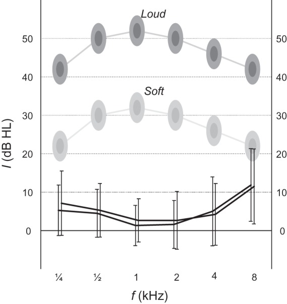
The error bars show tone thresholds at octave intervals from ¼ to 8 kHz for all subjects in both ears (mean ± SD; left ear: offset to the left; right ear: offset to the right). Shaded ellipses indicate the approximate intensity levels at which the employed stimuli were presented.

Sound-Evoked Activation Levels

Figure 3a shows the group-level activation to all sound stimuli, thresholded at a confidence level P < 0.05 (FWE corrected) and cluster size k > 100 voxels. Two large activation clusters were observed in the superior temporal lobe of the left and right hemispheres. These voxels were selected as an ROI and analyzed further. In Figure 3b, the activation levels of all voxels in the ROI in response to each of the 12 stimuli (expressed as a percentage signal change relative to baseline) are overlaid on an axial anatomical image by means of a color-coded mean intensity projection. All stimuli resulted in clear activation in the auditory cortices of both temporal lobes, perhaps with the exception of the soft 8-kHz condition. Unsurprisingly, the loud stimuli always resulted in stronger activation than the soft stimuli. Low-frequency stimuli also tended to result in stronger activation than high-frequency stimuli (although the ¼-kHz stimuli evoked slightly less activity than the ½- and 1-kHz stimuli). With regard to the spatial activation pattern, notable differences were observed between low- and high-frequency stimuli. Whereas low-frequency stimuli resulted in large activation clusters that occurred centrally laterally in the ROI and that peaked in lateral HG, the activation in response to high-frequency stimuli started to break up into 2 smaller clusters along the medial periphery of the ROI on the anterior and posterior sides of medial HG.

Figure 3.

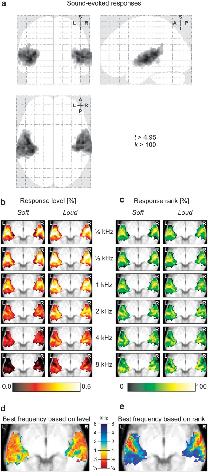
(a) Activation to all sound stimuli relative to silence according to a t-test thresholded at a confidence level P < 0.05 (FWE corrected) and cluster size k > 100 voxels. Two extensive activation clusters were observed in bilateral auditory cortex, which were subsequently used as an ROI. (b) For the sound stimuli of various frequencies (¼, ½, 1, 2, 4, or 8 kHz) and intensities (soft or loud), activation maps were constructed that display the response levels of all voxels in the ROI. (c) For each of the maps, voxels were rank ordered and percentile values are shown. (d) The frequency corresponding with the condition that resulted in the largest response level is mapped. (e) Similarly, the frequency corresponding with the condition that resulted in the largest response rank is mapped.

In order to be able to better appreciate the differences in the spatial organization of evoked activation without the presence of confounding differences in overall response magnitudes, the activation levels of all voxels in the ROI were rank ordered. For each of the 12 response vectors β, amplitudes were transformed such that the nth percentile voxel was assigned a value n (i.e., the least active voxel equaled 0, the most active voxel equaled 100, the median voxel equaled 50, and so forth). Results are shown in Figure 3c by means of a color-coded mean intensity projection. Differences between soft and loud stimuli largely disappeared (as compared with Fig. 3b). The activation maxima to low-frequency stimuli were clearly found to peak in one central location situated in lateral HG, while activation maxima to high-frequency stimuli gradually migrated toward the medial edge of the ROI, both in anterior and in posterior direction.

In Figure 3d–e, voxels were color-coded according to the frequency that resulted in the highest response level or response rank (irrespective of loudness), respectively. Best frequencies were averaged across voxels that overlap along the z-direction. Because low-frequency stimuli resulted in the largest absolute responses, these frequencies dominate in the map based on response levels. Still, high frequencies were encountered in a limited number of voxels that bordered anteriorly or posteriorly to HG, mostly in the medial half. Based on rank, however, high frequencies were much more abundant and dominated along the entire medial edge of the cluster, both anterior and posterior to HG.

To quantify the similarities between the various maps, (Pearson) correlation coefficients were calculated and displayed in Figure 4a. With regard to the correlations between soft stimuli mutually (lower left quadrant) or between loud stimuli mutually (upper right quadrant), the response maps to pairs of soft stimuli were always found to be correlated less strongly than those to the corresponding pair of loud stimuli. Furthermore, correlations strictly decreased as the difference in stimulus frequency became bigger (i.e., further from the diagonal). Both of these observations are illustrated in Figure 4b, where the correlation coefficients R between pairs of soft or loud stimuli are plotted as a function of the frequency difference Δf. This shows that the activation pattern to any particular frequency resembles the activation to neighboring frequencies but progressively less so for more distant frequencies. At the same time, response maps to soft stimuli were more dissimilar than those to corresponding loud stimuli. Figure 4a also shows that frequencies from ¼ to 2 kHz were all relatively highly correlated, whereas the 4- and 8-kHz stimuli correlated much less with any of the other frequencies.

Figure 4.

Activations of all voxels in the ROI were correlated between pairs of stimuli. (a) The diameters of the disks reflect the similarity between the response maps to stimuli of varying frequency and loudness, as indicated by the value of the (Pearson) correlation coefficient R. (b) For all pairs of distinct frequencies, correlations R between pairs of soft stimuli (light diamonds, dotted line) or pairs of loud stimuli (dark diamonds, solid line) are plotted as a function of the frequency difference Δf (expressed in octaves). Correlations decreased as stimulus frequencies differed more strongly. Moreover, response maps to soft stimuli were more dissimilar than those to loud stimuli.

With regard to the correlations between soft and loud stimuli (upper left and lower right quadrants), the highest correlations were again found near the diagonal. On top of that, a weak but systematic asymmetry could be observed. Soft stimuli at intermediate frequencies correlated better with loud stimuli at extreme frequencies than the other way around. For example, a soft 1-kHz stimulus and a loud ¼-kHz stimulus correlated more strongly than a loud 1-kHz stimulus and a soft ¼-kHz stimulus; also, a soft 2-kHz stimulus and a loud 8-kHz stimulus correlated more strongly than a loud 2-kHz stimulus and a soft 8-kHz stimulus.

Principal Components

The response matrix B was decomposed into principal components. The first principal component explained a proportion of 94.6% of the total signal power. The second component was 5.4 times weaker in root-mean-square sense and explained an additional 3.2%. The other components were much weaker still and each explained less than 0.5% (0.2 ± 0.1%, mean ± SD). On the basis of a scree test, the first 2 components were studied further.

The first principal component that best summarizes (in least squares sense) the observed response patterns across all activated voxels and all presented stimuli is shown in Figure 5a. The component's response map resembles Figure 3a and well summarizes the typical activation pattern in Figure 3b. The corresponding response profile also reveals the same trends that were already observed in Figure 3b: Most notably, response amplitudes increase with loudness and responses decline toward higher frequencies (except for ¼ kHz).

Figure 5.

Results of the principal component analysis. (a,b) The first and second principal components are shown, respectively. Maps show the principal component's amplitude as a function of voxel location, projected on an axial anatomical slice; bar graphs show the corresponding response profiles as a function of stimulus frequency and loudness. (c) The voxelwise amplitudes of the first and second principal component (A₁ and A₂) were compared. Their ratio A₂/A₁ is shown by means of a color-coded map; their values are plotted in a scatter plot. In (d), the same map is shown on a 3D mean cortical surface reconstruction, viewed from above (see also Supplementary Movie S1). For improved visibility of the superior surface of the temporal lobe, including HG, only the lower middle part of the brain is shown, sectioned through an oblique axial plane at 2z + y = 10. (e) The direction of the 2D gradient of the map in panel c was color-coded and plotted as a function of the x- and y-coordinates. In each hemisphere, 3 parallel strips were observed within which the gradient retained the same direction but across which it showed sudden jumps. (f) The histograms of the gradient directions in panel e showed a strongly bimodal distribution, which was highly comparable between the 2 hemispheres except for a mirroring around the y-axis.

Figure 5b similarly displays the second principal component, which summarizes how data primarily tend to deviate from the behavior shown in the first component alone. The response map contains negative values at the lateral extreme of HG (red) and positive values at the posterior and anterior borders of HG on its medial side (blue). The corresponding response profile shows a monotonous increase as a function of frequency, starting negative at ¼ kHz and ending positive at 8 kHz. Combined, this means that voxels are relatively more responsive to low-frequency stimulation in lateral HG and relatively more responsive to high-frequency stimuli in anteromedial and posteromedial HG.

Because the shape of the response profile that results from the first 2 principal components combined is determined by the relative contribution of the first and second component in a voxel, their strengths were compared and plotted in Figure 5c. The map shows a mean intensity projection of the ratio A₂/A₁, as calculated for each voxel; the scatter plot shows A₂ versus A₁, where every voxel contributes one data point. Both panels are color-coded according to the same scale. Qualitatively, the resulting map is somewhat similar to that in Figure 5b. High-frequency extrema were observed in posterior medial HG near (x, y, z) = (−44, −36, +10) and (+52, −28, +8) and anterior medial HG near (x, y, z) = (−30, −26, +8) and (+36, −22, +10); primary low-frequency extrema were located in lateral HG near (x, y, z) = (−56, −12, +2) and (+62, −4, +2) and weaker secondary extrema were found in lateral PT near (x, y, z) = (−62, −32, +10) and (+68, −22, +4).

Because in a mean intensity projection many voxels will overlap, in Figure 5d, the same map is shown on a 3D cortical surface cross-section instead. The color bar illustrates the shape of the response profiles that are obtained for various mixtures of the first 2 components. Again, negative values that reflect a low-frequency preference were observed at the lateral extreme of HG, which can be seen to run diagonally over the top of the temporal lobe, whereas positive values that reflect a high-frequency preference were found on the anterior and posterior banks of medial HG. To better convey the 3D layout, a supplementary animated figure is provided (Supplementary Movie S1).

In Figure 5e, the direction of the gradient of the A₂/A₁ ratio map (in Fig. 5c) is color coded. In each hemisphere, 3 parallel strips could be observed within which the gradient retained more or less the same direction but across which it showed sharp discontinuities. These comprised the rostral bank of HG (rHG), the caudal bank of HG (cHG), and the PT, respectively. In the left hemisphere, some evidence for another gradient reversal was apparent posteriorly, near the temporoparietal junction. Figure 5f plots a histogram of the observed directions across all voxels in the left and right hemispheres separately. Each histogram shows a bimodal distribution, with 2 peaks corresponding with the alternating parallel strips. Except for a mirror reversal in the midsagittal plane, the 2 hemispheres show a highly comparable distribution.

Individual Activation Patterns

So far, all results were derived from the mean group data. To ascertain that similar maps existed in individual subjects, the individual response level data of all ROI voxels were fitted with the first and second component's response profiles that are shown in Figure 5a,b (note that because the response profiles of all principal components are orthogonal, inclusion of the other response profiles into the fit is inconsequential). Figure 6 shows the resulting maps for all 20 subjects. The reported correlation coefficients R quantify the similarity between the individual subject map and the group map of the second component (shown in Fig. 5b). Overall, in spite of some intersubject variability, most individual maps well resembled the group map. With the exception of one subject that showed little or no sound-evoked activation at the subject level (bottom right, labeled “n3839” in the figure), correlations between maps were always positive and high in magnitude. The median R equaled 0.48.

Figure 6.

Individual maps corresponding with the group principal components were determined by fitting the individual voxel response level data with the response profiles belonging to the first and second principal components that were derived from the average group data. Color codes are the same as in Figure 5a,b. Correlation coefficients R quantify the similarities between the second component's maps of individuals and the group.

Discussion

In the present study, robust tonotopic maps were demonstrated in response to minimally salient tone stimuli in a group of 20 subjects. Six different stimulus frequencies were used, spanning a range of 5 octaves. In the derived activation maps, activation clusters could be seen to travel from lateral HG toward both the anterior and the posterior sides of medial HG as the stimulus frequency increased. This suggests the presence of at least 2 tonotopic progressions on the rostral and caudal banks of HG (rHG and cHG). A principal component analysis was carried out, which showed that in our results, after variations in overall activation level that were captured by the first component, systematic differences in frequency preferences were the most dominant response feature. The corresponding component map captured the 2 tonotopic progressions that were already observed in the set of activation maps in closer detail but also revealed at least a third tonotopic progressions in PT. Moreover, multiple cortical regions could be clearly distinguished on the basis of tonotopic gradient direction. Finally, we showed that the observed behavior at the group level could be traced back to similar tonotopic mappings in individuals quite consistently.

Spatial Specificity

In the past, tonotopic progressions have often been demonstrated by following the trajectory of a single activation peak as a function of frequency or by comparing response profiles along a chosen curve across the cortical surface. These methods are relatively sensitive to noise, since outcomes are determined by the signals of only a small subset of voxels. Also, some subjectivity is introduced, for example, in the choice which local maxima to consider or where to draw the curve. Other approaches that capture the behavior of all voxels in one summary outcome, for instance by tracking the location of a cluster's “center of mass” as a function of frequency, have as a drawback that they have difficulty dealing with multiple tonotopic progressions simultaneously, especially when oppositely directed. We were able to avoid these limitations by looking at correlations between activation maps to quantify their similarities. We proved that frequency progressions are gradual by showing that similarities progressively decreased as frequency differences became larger. In combination with the fact that activation smoothly varies over space, we see little alternative then to conclude that tonotopic representations also map frequency onto the cortical surface in a gradual continuous manner.

We used task-irrelevant unattended sound stimuli. Attention is known to modulate activation levels, even at the level of primary auditory cortex (Palmer et al. 2007; Poghosyan and Ioannides 2008). We controlled for attention by involving our subjects in a nonauditory task. By engaging them in this manner, we hoped to remove potential effects of attention to the auditory stimuli. A parallel may exist between this controlled diversion and the use of anaesthetization, making our results more readily comparable to those from animal studies.

To further avoid excessive spread of activation across the auditory cortex, 2 stimulus intensities were employed that were relatively low but that differed by 20 dB. Comparing the sound-evoked activations, clear evidence was indeed found that activation was more extensive and spatially less specific for the louder set of stimuli than for the softer set. Activation patterns that were related to different frequencies resembled each other more closely for loud stimuli than for corresponding soft stimuli (Fig. 4b). Moreover, the response maps to low frequencies, which were presented furthest above threshold, were more strongly correlated than those for the highest frequencies, which were presented closer to the hearing threshold. This cannot simply be explained by an overall difference in activation magnitude, as observed in the activation maps for instance, because correlations are insensitive to scale. Instead, our results indicate that activations to loud stimuli show more spatial overlap than those to low intensities. Such an increase in overlap may either result from activations becoming more extensive or from activations moving closer together. When cross-correlating the activations to soft and loud stimuli, we observed that activations to same-frequency stimuli remained highly correlated. This suggests that the observed increase in overlap should be largely attributed to enlarged activation extents, that is, spread of activation. Nevertheless, a systematic trend was observed that suggested that low- and high-frequency activations at high levels had shifted toward the middle frequencies to some extent. However, this effect was weak and can be understood for instance if spread of activation toward neighboring frequencies occurs for the extremest frequencies but cannot continue beyond the endpoints that limit the tonotopic map and is therefore forced toward intermediate frequency regions.

The disclosed spread of activation may have occurred on a neural level. Excitation patterns are known to spread in asymmetrical fashion in the cochlea already. However, this always occurs in the form of a net shift toward the low-frequency tonotopic endpoint (Recanzone et al. 2000). We did observe such a trend for high-frequency stimuli, but if anything the opposite was seen for low frequencies. Still, such spread may arise more centrally in the auditory system, since lateral projections between neurons that respond to neighboring frequencies abound at various levels (Schreiner et al. 2000). Alternatively, an explanation may be sought in hemodynamics. As metabolic demand in the brain locally increases, capillaries become more dilated, but at the same time, more capillaries are recruited. In combination with the sensitivity for downstream venous effects in BOLD fMRI, increased activation conceivably leads to apparent recruitment of a larger cortical area. However, regardless whether the spread of activation is a result of neural or hemodynamic mechanisms, our findings prove that the most accurate and spatially specific tonotopic maps may be obtained with fMRI using low-level stimuli (provided that responses can still be confidently detected).

Tonotopic Maps

Our results clearly showed that the low-frequency stimuli evoked strong responses especially in a central lateral location in the detected acoustically responsive superior temporal lobe. In contrast, high-frequency stimuli were seen to activate regions medially toward the periphery of the activation cluster. Upon closer inspection, 2 separate high-frequency endpoints could be distinguished, 1 on the posterior side of medial HG and 1 on its anterior side. This gives rise to 2 tonotopic frequency progressions, separated by the crest of HG, and covering the caudal and rostral half of HG, respectively. These 2 regions could also be clearly distinguished on the basis of the local frequency gradient's direction, which remained relatively constant within regions but suddenly changed at their boundary. Notably, these gradients were not colinear and antiparallel but set at a pronounced angle. We hypothesize that these tonotopic maps correspond with functional fields in auditory cortex, illustrated and labeled cHG and rHG in Figure 7a. The principal component analysis revealed a posterior secondary low-frequency endpoint, which was accompanied by another gradient reversal. This points at the existence of an additional tonotopic gradient in the PT (Fig. 7a).

Figure 7.

(a) The tonotopic layout was visualized by means of iso-frequency contour plots (white lines) and interpreted in terms of putative boundaries between auditory fields (black lines). Three tonotopic progressions were identified on rHG, cHG, and PT. Endpoints showing low- and high-frequency responses are indicated by filled circles (L and H, respectively). (b) Prominent anatomical features in the region of the auditory cortex comprise the insula (INS), circular sulcus (CS), planum polare (PP), HG, Heschl's sulcus (HS), PT, and temporoparietal junction (TPJ). Labels are overlaid on a rendering of the left superior temporal surface, as outlined by dashed lines in panel a. (c) Numerous neuroimaging studies have revealed an effective tonotopic gradient extending from anterolateral to posteromedial HG (see the Introduction). (d–g) Tonotopic endpoints that were obtained in other studies are reproduced in a similar view to facilitate comparisons. Numbered endpoints correspond with identically numbered endpoints in the original publications. (h–k) A number of cortical parcellation schemes for the region of the human auditory cortex were proposed in the literature. Areas: Kl: lateral koniocortex, Km: medial koniocortex, PaAc/r/i/e: caudal/rostral/internal/external parakoniocortical, Reit: retroinsular, Tpt: temporoparietal, Ts: superior temporal, and ProK: prokoniocortex; LP: lateroposterior, AI: primary auditory, PA: posterior, LA: lateral, STA: superior temporal, ALA: anterior lateral, AA: anterior, and MA: medial; Te1.0/1.1/1.2/2/3: temporal 1.0/1.1/1.2/2/3, and TI1: temporoinsular 1; A1: primary auditory, R: rostral, RT: rostrotemporal, CL: caudolateral, CM: caudomedial, ML: middle lateral, MM: middle medial, AL: anterolateral, RM: rostromedial, RTL: lateral rostrotemporal, and RTM: medial rostrotemporal. Consult the original publications for further details regarding these cortical activation patterns and parcellation schemes.

With regard to neuroimaging results in humans, the outcomes of past studies are inconsistent and sometimes even appear contradictory. Nevertheless, our results are retrospectively compatible with the vast majority of literature and may thus serve to reconcile many of the published findings. Without claiming to be exhaustive, we shall compare our results with a number of influential studies that we consider representative.

Many EEG/MEG as well as PET/fMRI studies (see the Introduction) were able to show that low frequencies are mapped to lateral HG, whereas high frequencies are mapped to more medial regions of HG. This is schematically depicted in Figure 7c. Such an organization is completely consistent with ours when realizing that for various methodological reasons the spatial resolution of these studies was often limited. This may easily have led the 2 nearby medial high-frequency endpoints to be grouped, resulting in a single gradient that is well aligned with the axis of HG.

The known existence of abutting frequency gradients in monkeys has led researchers to subsequently look for evidence for a second colinear mirrored tonotopic map in lateral HG. One of the first studies that seemed to unambiguously confirm such an organization was reported by Formisano et al. (2003). These authors considered the frequency selectivity along a curve that ran along HG and indeed found a characteristic high-to-low-to-high reversal of best frequency (Fig. 7d). However, their curve also gradually crossed from the caudal bank of HG in medial locations (endpoint “a” in their labeling) to its rostral bank on the lateral side (endpoint “f”) and at least partially traversed both the cHG and the rHG fields as identified by us. For that reason, their frequency progressions are not incompatible with ours. In their publication, the authors did not report a high-frequency endpoint in medial rostral HG, possibly because significant signal was not always detected in that region or because the employed cortical unfolding may have made it appear as if it concerned the same endpoint as the caudal one or perhaps because animal studies did not suggest the existence of such an endpoint and they therefore did not seek it out. Whatever the reason, retrospectively, evidence for such an endpoint was present in the published data (for instance in their subject #5 shown in their Fig. 5b). This leads us to conclude that although our interpretation differs from theirs, in particular regarding the location and orientation of the second tonotopic map, our underlying results are not inconsistent.

In the same period, Talavage et al. (2000, 2004) published a pair of studies that painted a different picture compared with that from Formisano and colleagues (Fig. 7e). Seven or 8 low- and high-frequency endpoints were identified (in 2004 and 2000, respectively), connected by up to 6 tonotopic progressions (in 2004). Because of the large number of tonotopic maps, an unambiguous correspondence with those in our study is not straightforward to establish. Still, 3 of their progressions were observed in all subjects without exception: one running from endpoint 1′ on lateral HG to endpoint 2′ on anteromedial HG; one running from endpoint 1′ on lateral HG to endpoint 3′ on posterior HG; and one running from endpoint 6′ on lateral superior temporal gyrus to endpoint 3′ on posterior HG. This pattern is reminiscent of the 3 tonotopic progressions that we observed in rHG, cHG, and PT. Although the high-frequency endpoints 2′ and 3′ were not located at the root of HG, we note that in the earlier paper, endpoint 2 actually was positioned almost 1 cm more medially and an additional endpoint numbered 4 was found on medial caudal HG. Differences between those 2 studies may have arisen due to the use of surface coils, with limited sensitivity in medial locations. Furthermore, in all subjects except one, an additional progression was reported running from endpoint 8′ on PT to endpoint 3′ on posterior HG. If endpoints 3/3′ and 4 can be attributed to the same high-frequency region and endpoints 6/6′ and 8/8′ to the same low-frequency region, then both the pattern and the locations of the tonotopic progressions are compatible with what we observed. Again, individual subject data resulted in patterns that were reasonably compatible with our own (for instance subjects #2 and #6 in Fig. 4 of the 2004 paper). Two more gradients were reported to occur in two-thirds of the subjects. One was found more anteriorly, from 7′ to 2′; we were unable to distinguish this as a separate gradient in our data. Another one was found more laterally, from 6′ to 5′; we did not find any high-frequency preference in that vicinity. Still, the layout of the most prominent tonotopic maps can be brought into agreement with our results.

Schönwiesner et al. (2002) published a study in which a number of low- and high-frequency endpoints were reported (Fig. 7f), numbered analogously to those of Talavage and co-workers. They identified 2 separate high-frequency endpoints (2 and 4) in medial HG and further distinguished 2 more lateral low-frequency endpoints that they both interpreted to be derived from endpoint 1/1′ in Talavage's study. Although in our study, we did not discriminate 2 such low-frequency endpoints, their existence is compatible with the existence of a dual tonotopic map in cHG and rHG. Also, additional endpoints (3 and 8) were found on the PT, suggesting a tonotopic gradient in that region that is similarly aligned to ours. However, Schönwiesner et al. did not interpret their findings in terms of tonotopic maps. Instead, they suggested that low- or high-frequency responses might reflect different types of processing, which just happen to rely on information from different spectral domains. They came to this conclusion primarily because they observed differences between low- and high-frequency responses but not between pairs of either low (¼ and ½ kHz) or high (4 and 8 kHz) frequencies. Unfortunately, in their study, no intermediate frequencies (e.g., 1 and 2 kHz) were included. Possibly, the use of an auditory task, moderately loud frequency-modulated stimuli, the effects of scanner noise, and reliance on observable shifts in activation peaks, conspired to hide the differences between activation patterns that resulted from stimuli that differed by merely one octave. In our study, we did include all aforementioned frequencies and found progressively less similar response patterns as frequencies differed more strongly. In particular, we did not observe a discrete change at some intermediate transition frequency. We therefore conclude that an interpretation in terms of continuous tonotopic organizations within cortical fields is more obvious than an interpretation in terms of discrete differences in preferred frequencies between such fields.

More recently, Humphries et al. (2010) published tonotopic maps that closely resembled ours. Although they did not present their results in terms of low- and high-frequency endpoints, for ease of comparison, we plotted the location of apparent local frequency extrema in Figure 7g (this representation was derived from their Fig. 6). Similarly to our results, in this work 2 distinct high-frequency endpoints were observed rostrally and caudally near medial HG. Low-frequency activation clustered on lateral HG and spread anteriorly and posteriorly along lateral superior temporal gyrus, with a second low-frequency peak in PT. They interpreted their results to contain 2 mirrored tonotopic maps that ran more or less perpendicular to HG. The emerging picture is quite consistent with that in monkeys (Petkov et al. 2006, 2009; Tanji et al. 2010) and the anterior of these maps also agrees with some earlier MEG results in humans (Ozaki and Hashimoto 2007). Two other studies reported a somewhat similar organization using fMRI in humans (Woods et al. 2009; Striem-Amit et al. 2011), although the suggested tonotopic axes in these studies ran more or less diagonally and colinearly across HG, in an orientation that was intermediate between those of Formisano et al. (2003) and Humphries et al. (2010). Still, high-frequency responses in rostral HG were found medially as well. Our results appear to be consistent with these recent findings.

Cortical Organization

Tonotopic maps are thought to correspond with cortical fields. Consequently, borders between neighboring tonotopic progressions may serve to identify boundaries between such fields. This idea has already been established in the visual system, where a distinction between fields is made on the basis of retinotopic reversals (Engel et al. 1997), and it is now gaining importance for the auditory system as well (Petkov et al. 2006; Woods et al. 2010). In this study, we observed sharp transitions in tonotopic gradient direction. Therefore, it is of interest to compare our functional outcomes with parcellations that have been proposed on the basis of, for example, cytoarchitectonic and histochemical criteria (Hall et al. 2003). Cortical organization has been investigated since the beginning of the previous century already (Brodmann 1909; von Economo and Koskinas 1925). In Figure 7, we have attempted to summarize 4 parcellations of auditory cortex that were arrived at in recent times.

Figure 7h depicts a simplified parcellation based on Fullerton and Pandya (2007) and preceding work (Pandya and Sanides 1973; Galaburda and Sanides 1980; Galaburda and Pandya 1983). A distinction is made between a “core” region on the superior temporal surface, a more medial “root” region near the circular sulcus, and a more lateral “belt” region in superior temporal gyrus. In the core, 2 koniocortical fields can be distinguished, 1 laterally and 1 medially (the latter of which has further been subdivided by these authors). These areas are surrounded by lateral rostral and caudal parakoniocortical fields. The root consists of retroinsular, proisocortical, and prokoniocortical areas and the belt consists of at least the lateral (external) parts of superior temporal, parakoniocortical, and temporoparietal areas. Based on their position and orientation, our tonotopic gradients in rostral and caudal HG should be identified with medial and lateral koniocortex, respectively, while the progression in PT may correspond with one of the parakoniocortical fields.

Figure 7i shows a subdivision based on histological staining that was originally arrived at by Rivier and Clarke and subsequently refined by Wallace (Rivier and Clarke 1997; Clarke and Rivier 1998; Wallace et al. 2002). The posteromedial two-thirds of HG are covered by a field named A1. Its cytochemical characteristics (e.g., dense cytochrome oxidase staining in layer IV) suggest that it is a primary sensory area that receives main input from thalamic afferents. By using additional stains, Wallace et al. (2002) further discriminated a lateroposterior area, running parallel and adjacent to A1 in the bank of the Heschl’s sulcus, which was also interpreted to belong to the auditory core region. These 2 areas are highly similar to the medial and lateral koniocortical areas by Fullerton and Pandya (2007) and may equally be identified with our rostral and caudal HG. Surrounding these core areas, around 6 other auditory areas were identified. Two caudal areas, named the posterior and lateral area, may host the tonotopic gradient in PT.

Using an observer-independent method to define borders between cortical areas, Morosan et al. (2001) identified a koniocortical primary auditory region Te1 (Rademacher et al. 2001; Bailey et al. 2007; Schleicher et al. 2009). This was subdivided into 3 divisions along the extent of HG in the posteromedial to anterolateral direction, labeled Te1.1, Te1.0, and Te1.2, respectively. On the basis of its wide layer IV, area Te1.0 was interpreted to receive the largest number of thalamic projections. Te1 is bordered posteriorly by area Te2, laterally by Te3, and anteriorly by TI1. Although our observation of the 3 regions in auditory cortex might point to a correspondence between rHG and TI1, between cHG and Te1, and between PT and Te2, the location and extent of these areas suggest that both rHG and cHG fall inside Te1. The subdivision of Te1 into Te1.1, Te1.0, and Te1.2 does not agree very well with our subdivision of HG in rHG and cHG. Morosan et al. (2001) suggested that Te1 may contain one tonotopic progression. The high frequencies would then be represented in Te1.1 and the low frequencies in Te1.2. The intermediate frequencies that are important for speech might be processed in Te1.0. Given that we observed the tonotopic gradient to have a strong component perpendicular to the axis of HG, we suspect that the represented frequencies overlap between these subdivisions. According to our results, an additional distinction between the caudal and the rostral side of Te1 should be made.

Figure 7k shows a parcellation that has been established in monkeys and that has been suggested to exist in humans in homologous form (Sweet et al. 2005). A tonotopic correspondence was already pointed out in the publications by Woods et al. (2009) and Humphries et al. (2010). This parcellation also includes a primary core region, which is subdivided into 2 areas, AI and R (Merzenich and Brugge 1973; Imig et al. 1977; Morel et al. 1993) and possibly a third area RT (Morel and Kaas 1992; Rauschecker et al. 1997; Hackett et al. 1998; Kaas and Hackett 2000). These are all tonotopically organized with mirrored abutting frequency gradients set at a distinct angle. Because this closely resembles the organization that we observed, we identify rHG with area R and cHG with AI. Surrounding secondary “belt” and “parabelt” regions contain several additional areas, some of which are tonotopically organized as well (Striem-Amit et al. 2011). Because the orientation of their tonotopic maps tend to match those of neighboring core regions seamlessly (Kusmierek and Rauschecker 2009; Woods and Alain 2009), we may have been unable to distinguish between such core and belt areas on the basis of our functional outcomes alone. The third tonotopic gradient that we observed in PT coincides with the caudal areas CL and CM.

In summary, although the various parcellations differ in various respects, they tend to agree on the existence of a primary auditory core region in medial HG that consists of at least 2 subdivisions, which are often aligned parallel on the rostral and caudal side of the axis of HG. Such an organization is highly compatible with the dual tonotopic progressions that were observed in this study.

Supplementary Material

Supplementary material can be found at: http://www.cercor.oxfordjournals.org/

Funding

The author D.R.M.L. was funded by VENI research grant 016.096.011 from the Netherlands Organisation for Scientific Research (NWO) and the Netherlands Organization for Health Research and Development (ZonMw). Further financial support was provided by the Heinsius Houbolt Foundation.

References

- Ahveninen J, Hämäläinen M, Jääskeläinen IP, Ahlfors SP, Huang S, Lin F-H, Raij T, Sams M, Vasios CE, Belliveau JW. Attention-driven auditory cortex short-term plasticity helps segregate relevant sounds from noise. Proc Natl Acad Sci U S A. 2011;108:4182–4187. doi: 10.1073/pnas.1016134108. [DOI] [PMC free article] [PubMed] [Google Scholar]
- Bailey L, Abolmaesumi P, Tam J, Morosan P, Cusack R, Amunts K, Johnsrude I. Customised cytoarchitectonic probability maps using deformable registration: primary auditory cortex. Med Image Comput Comput Assist Interv. 2007;10:760–768. doi: 10.1007/978-3-540-75759-7_92. [DOI] [PubMed] [Google Scholar]
- Baumgart F, Kaulisch T, Tempelmann C, Gaschler-Markefski B, Tegeler C, Schindler F, Stiller D, Scheich H. Electrodynamic headphones and woofers for application in magnetic resonance imaging scanners. Med Phys. 1998;25:2068–2070. doi: 10.1118/1.598368. [DOI] [PubMed] [Google Scholar]
- Bidet-Caulet A, Fischer C, Besle J, Aguera P-E, Giard M-H, Bertrand O. Effects of selective attention on the electrophysiological representation of concurrent sounds in the human auditory cortex. J Neurosci. 2007;27:9252–9261. doi: 10.1523/JNEUROSCI.1402-07.2007. [DOI] [PMC free article] [PubMed] [Google Scholar]
- Bilecen D, Scheffler K, Schmid N, Tschopp K, Seelig J. Tonotopic organization of the human auditory cortex as detected by BOLD-FMRI. Hear Res. 1998;126:19–27. doi: 10.1016/s0378-5955(98)00139-7. [DOI] [PubMed] [Google Scholar]
- Brodmann K. Vergleichende Loakalisationslehre der Grosshirnrinde. Leipzig (Germany): JA Barth; 1909. [Google Scholar]
- Cansino S, Williamson SJ, Karron D. Tonotopic organization of human auditory association cortex. Brain Res. 1994;663:38–50. doi: 10.1016/0006-8993(94)90460-x. [DOI] [PubMed] [Google Scholar]
- Capsius B, Leppelsack H. Response patterns and their relationship to frequency analysis in auditory forebrain centers of a songbird. Hear Res. 1999;136:91–99. doi: 10.1016/s0378-5955(99)00112-4. [DOI] [PubMed] [Google Scholar]
- Clarke S, Rivier F. Compartments within human primary auditory cortex: evidence from cytochrome oxidase and acetylcholinesterase staining. Eur J Neurosci. 1998;10:741–745. doi: 10.1046/j.1460-9568.1998.00043.x. [DOI] [PubMed] [Google Scholar]
- Cohen YE, Knudsen EI. Representation of frequency in the primary auditory field of the barn owl forebrain. J Neurophysiol. 1996;76:3682–3692. doi: 10.1152/jn.1996.76.6.3682. [DOI] [PubMed] [Google Scholar]
- Engel SA, Glover GH, Wandell BA. Retinotopic organization in human visual cortex and the spatial precision of functional MRI. Cereb Cortex. 1997;7:181–192. doi: 10.1093/cercor/7.2.181. [DOI] [PubMed] [Google Scholar]
- Engelien A, Yang Y, Engelien W, Zonana J, Stern E, Silbersweig DA. Physiological mapping of human auditory cortices with a silent event-related fMRI technique. Neuroimage. 2002;16:944–953. doi: 10.1006/nimg.2002.1149. [DOI] [PubMed] [Google Scholar]
- Formisano E, Kim DS, Di Salle F, van de Moortele PF, Ugurbil K, Goebel R. Mirror-symmetric tonotopic maps in human primary auditory cortex. Neuron. 2003;40:859–869. doi: 10.1016/s0896-6273(03)00669-x. [DOI] [PubMed] [Google Scholar]
- Fritz J, Shamma S, Elhilali M, Klein D. Rapid task-related plasticity of spectrotemporal receptive fields in primary auditory cortex. Nat Neurosci. 2003;6:1216–1223. doi: 10.1038/nn1141. [DOI] [PubMed] [Google Scholar]
- Fullerton BC, Pandya DN. Architectonic analysis of the auditory-related areas of the superior temporal region in human brain. J Comp Neurol. 2007;504:470–498. doi: 10.1002/cne.21432. [DOI] [PubMed] [Google Scholar]
- Gabriel D, Veuillet E, Ragot R, Schwartz D, Ducorps A, Norena A, Durrant JD, Bonmartin A, Cotton F, Collet L. Effect of stimulus frequency and stimulation site on the N1m response of the human auditory cortex. Hear Res. 2004;197:55–64. doi: 10.1016/j.heares.2004.07.015. [DOI] [PubMed] [Google Scholar]
- Galaburda A, Sanides F. Cytoarchitectonic organization of the human auditory cortex. J Comp Neurol. 1980;190:597–610. doi: 10.1002/cne.901900312. [DOI] [PubMed] [Google Scholar]
- Galaburda AM, Pandya DN. The intrinsic architectonic and connectional organization of the superior temporal region of the rhesus monkey. J Comp Neurol. 1983;221:169–184. doi: 10.1002/cne.902210206. [DOI] [PubMed] [Google Scholar]
- Hackett TA, Stepniewska I, Kaas JH. Subdivisions of auditory cortex and ipsilateral cortical connections of the parabelt auditory cortex in macaque monkeys. J Comp Neurol. 1998;394:475–495. doi: 10.1002/(sici)1096-9861(19980518)394:4<475::aid-cne6>3.0.co;2-z. [DOI] [PubMed] [Google Scholar]
- Hall DA, Hart HC, Johnsrude IS. Relationships between human auditory cortical structure and function. Audiol Neurootol. 2003;8:1–18. doi: 10.1159/000067894. [DOI] [PubMed] [Google Scholar]
- Hellweg FC, Koch R, Vollrath M. Representation of the cochlea in the neocortex of guinea pigs. Exp Brain Res. 1977;29:467–474. doi: 10.1007/BF00236184. [DOI] [PubMed] [Google Scholar]
- Hertz U, Amedi A. Disentangling unisensory and multisensory components in audiovisual integration using a novel multifrequency fMRI spectral analysis. Neuroimage. 2010;52:617–632. doi: 10.1016/j.neuroimage.2010.04.186. [DOI] [PubMed] [Google Scholar]
- Howard MA, Volkov IO, Abbas PJ, Damasio H, Ollendieck MC, Granner MA. A chronic microelectrode investigation of the tonotopic organization of human auditory cortex. Brain Res. 1996;724:260–264. doi: 10.1016/0006-8993(96)00315-0. [DOI] [PubMed] [Google Scholar]
- Humphries C, Liebenthal E, Binder JR. Tonotopic organization of human auditory cortex. Neuroimage. 2010;50:1202–1211. doi: 10.1016/j.neuroimage.2010.01.046. [DOI] [PMC free article] [PubMed] [Google Scholar]
- Huotilainen M, Tiitinen H, Lavikainen J, Ilmoniemi RJ, Pekkonen E, Sinkkonen J, Laine P, Näätänen R. Sustained fields of tones and glides reflect tonotopy of the auditory cortex. Neuroreport. 1995;6:841–844. doi: 10.1097/00001756-199504190-00004. [DOI] [PubMed] [Google Scholar]
- Imig TJ, Ruggero MA, Kitzes LM, Javel E, Brugge JF. Organization of auditory cortex in the owl monkey (Aotus trivirgatus) J Comp Neurol. 1977;171:111–128. doi: 10.1002/cne.901710108. [DOI] [PubMed] [Google Scholar]
- Kaas JH, Hackett TA. Subdivisions of auditory cortex and processing streams in primates. Proc Natl Acad Sci U S A. 2000;97:11793–11799. doi: 10.1073/pnas.97.22.11793. [DOI] [PMC free article] [PubMed] [Google Scholar]
- Kelly JB, Judge PW, Phillips DP. Representation of the cochlea in primary auditory cortex of the ferret (Mustela putorius) Hear Res. 1986;24:111–115. doi: 10.1016/0378-5955(86)90054-7. [DOI] [PubMed] [Google Scholar]
- Kuriki S, Murase M. Neuromagnetic study of the auditory responses in right and left hemispheres of the human brain evoked by pure tones and speech sounds. Exp Brain Res. 1989;77:127–134. doi: 10.1007/BF00250574. [DOI] [PubMed] [Google Scholar]
- Kusmierek P, Rauschecker JP. Functional specialization of medial auditory belt cortex in the alert rhesus monkey. J Neurophysiol. 2009;102:1606–1622. doi: 10.1152/jn.00167.2009. [DOI] [PMC free article] [PubMed] [Google Scholar]
- Lang PJ, Bradley MM, Cuthbert BN. International Affective Picture System (IAPS): affective ratings of pictures and instruction manual. 2008. Technical Report A-8. Gainesville, FL: University of Florida. [Google Scholar]
- Langers DRM, Backes WH, van Dijk P. Representation of lateralization and tonotopy in primary versus secondary human auditory cortex. Neuroimage. 2007;34:264–273. doi: 10.1016/j.neuroimage.2006.09.002. [DOI] [PubMed] [Google Scholar]
- Lauter JL, Herscovitch P, Formby C, Raichle ME. Tonotopic organization in human auditory cortex revealed by positron emission tomography. Hear Res. 1985;20:199–205. doi: 10.1016/0378-5955(85)90024-3. [DOI] [PubMed] [Google Scholar]
- Le TH, Patel S, Roberts TP. Functional MRI of human auditory cortex using block and event-related designs. Magn Reson Med. 2001;45:254–260. doi: 10.1002/1522-2594(200102)45:2<254::aid-mrm1034>3.0.co;2-j. [DOI] [PubMed] [Google Scholar]
- Lockwood AH, Salvi RJ, Coad ML, Arnold SA, Wack DS, Murphy BW, Burkard RF. The functional anatomy of the normal human auditory system: responses to 0.5 and 4.0 kHz tones at varied intensities. Cereb Cortex. 1999;9:65–76. doi: 10.1093/cercor/9.1.65. [DOI] [PubMed] [Google Scholar]
- Luethke LE, Krubitzer LA, Kaas JH. Connections of primary auditory cortex in the New World monkey, Saguinus. J Comp Neurol. 1989;285:487–513. doi: 10.1002/cne.902850406. [DOI] [PubMed] [Google Scholar]
- McMullen NT, Glaser EM. Tonotopic organization of rabbit auditory cortex. Exp Neurol. 1982;75:208–220. doi: 10.1016/0014-4886(82)90019-x. [DOI] [PubMed] [Google Scholar]
- Merzenich MM, Brugge JF. Representation of the cochlear partition of the superior temporal plane of the macaque monkey. Brain Res. 1973;50:275–296. doi: 10.1016/0006-8993(73)90731-2. [DOI] [PubMed] [Google Scholar]
- Merzenich MM, Kaas JH, Roth GL. Auditory cortex in the grey squirrel: tonotopic organization and architectonic fields. J Comp Neurol. 1976;166:387–401. doi: 10.1002/cne.901660402. [DOI] [PubMed] [Google Scholar]
- Morel A, Garraghty PE, Kaas JH. Tonotopic organization, architectonic fields, and connections of auditory cortex in macaque monkeys. J Comp Neurol. 1993;335:437–459. doi: 10.1002/cne.903350312. [DOI] [PubMed] [Google Scholar]
- Morel A, Kaas JH. Subdivisions and connections of auditory cortex in owl monkeys. J Comp Neurol. 1992;318:27–63. doi: 10.1002/cne.903180104. [DOI] [PubMed] [Google Scholar]
- Morosan P, Rademacher J, Schleicher A, Amunts K, Schormann T, Zilles K. Human primary auditory cortex: cytoarchitectonic subdivisions and mapping into a spatial reference system. Neuroimage. 2001;13:684–701. doi: 10.1006/nimg.2000.0715. [DOI] [PubMed] [Google Scholar]
- Ozaki I, Hashimoto I. Human tonotopic maps and their rapid task-related changes studied by magnetic source imaging. Can J Neurol Sci. 2007;34:146–153. doi: 10.1017/s0317167100005965. [DOI] [PubMed] [Google Scholar]
- Palmer AR, Hall DA, Sumner C, Barrett DJK, Jones S, Nakamoto K, Moore DR. Some investigations into non-passive listening. Hear Res. 2007;229:148–157. doi: 10.1016/j.heares.2006.12.007. [DOI] [PubMed] [Google Scholar]
- Paltoglou AE, Sumner CJ, Hall DA. Mapping feature-sensitivity and attentional modulation in human auditory cortex with functional magnetic resonance imaging. Eur J Neurosci. 2011;33:1733–1741. doi: 10.1111/j.1460-9568.2011.07656.x. [DOI] [PMC free article] [PubMed] [Google Scholar]
- Pandya DN, Sanides F. Architectonic parcellation of the temporal operculum in rhesus monkey and its projection pattern. Z Anat Entwicklungsgesch. 1973;139:127–161. doi: 10.1007/BF00523634. [DOI] [PubMed] [Google Scholar]
- Pantev C, Bertrand O, Eulitz C, Verkindt C, Hampson S, Schuierer G, Elbert T. Specific tonotopic organizations of different areas of the human auditory cortex revealed by simultaneous magnetic and electric recordings. Electroencephalogr Clin Neurophysiol. 1995;94:26–40. doi: 10.1016/0013-4694(94)00209-4. [DOI] [PubMed] [Google Scholar]
- Pantev C, Eulitz C, Elbert T, Hoke M. The auditory evoked sustained field: origin and frequency dependence. Electroencephalogr Clin Neurophysiol. 1994;90:82–90. doi: 10.1016/0013-4694(94)90115-5. [DOI] [PubMed] [Google Scholar]
- Pantev C, Hoke M, Lehnertz K, Lütkenhöner B, Anogianakis G, Wittkowski W. Tonotopic organization of the human auditory cortex revealed by transient auditory evoked magnetic fields. Electroencephalogr Clin Neurophysiol. 1988;69:160–170. doi: 10.1016/0013-4694(88)90211-8. [DOI] [PubMed] [Google Scholar]
- Petkov CI, Kang X, Alho K, Bertrand O, Yund EW, Woods DL. Attentional modulation of human auditory cortex. Nat Neurosci. 2004;7:658–663. doi: 10.1038/nn1256. [DOI] [PubMed] [Google Scholar]
- Petkov CI, Kayser C, Augath M, Logothetis NK. Functional imaging reveals numerous fields in the monkey auditory cortex. PLoS Biol. 2006;4:e215. doi: 10.1371/journal.pbio.0040215. [DOI] [PMC free article] [PubMed] [Google Scholar]
- Petkov CI, Kayser C, Augath M, Logothetis NK. Optimizing the imaging of the monkey auditory cortex: sparse vs. continuous fMRI. Magn Reson Imaging. 2009;27:1065–1073. doi: 10.1016/j.mri.2009.01.018. [DOI] [PubMed] [Google Scholar]
- Poghosyan V, Ioannides AA. Attention modulates earliest responses in the primary auditory and visual cortices. Neuron. 2008;58:802–813. doi: 10.1016/j.neuron.2008.04.013. [DOI] [PubMed] [Google Scholar]
- Rademacher J, Morosan P, Schormann T, Schleicher A, Werner C, Freund HJ, Zilles K. Probabilistic mapping and volume measurement of human primary auditory cortex. Neuroimage. 2001;13:669–683. doi: 10.1006/nimg.2000.0714. [DOI] [PubMed] [Google Scholar]
- Rauschecker JP, Tian B, Pons T, Mishkin M. Serial and parallel processing in rhesus monkey auditory cortex. J Comp Neurol. 1997;382:89–103. [PubMed] [Google Scholar]
- Reale RA, Imig TJ. Tonotopic organization in auditory cortex of the cat. J Comp Neurol. 1980;192:265–291. doi: 10.1002/cne.901920207. [DOI] [PubMed] [Google Scholar]
- Recanzone GH, Guard DC, Phan ML. Frequency and intensity response properties of single neurons in the auditory cortex of the behaving macaque monkey. J Neurophysiol. 2000;83:2315–2331. doi: 10.1152/jn.2000.83.4.2315. [DOI] [PubMed] [Google Scholar]
- Rivier F, Clarke S. Cytochrome oxidase, acetylcholinesterase, and NADPH-diaphorase staining in human supratemporal and insular cortex: evidence for multiple auditory areas. Neuroimage. 1997;6:288–304. doi: 10.1006/nimg.1997.0304. [DOI] [PubMed] [Google Scholar]
- Romani GL, Williamson SJ, Kaufman L. Tonotopic organization of the human auditory cortex. Science. 1982;216:1339–1340. doi: 10.1126/science.7079770. [DOI] [PubMed] [Google Scholar]
- Scarff CJ, Dort JC, Eggermont JJ, Goodyear BG. The effect of MR scanner noise on auditory cortex activity using fMRI. Hum Brain Mapp. 2004;22:341–349. doi: 10.1002/hbm.20043. [DOI] [PMC free article] [PubMed] [Google Scholar]
- Schleicher A, Morosan P, Amunts K, Zilles K. Quantitative architectural analysis: a new approach to cortical mapping. J Autism Dev Disord. 2009;39:1568–1581. doi: 10.1007/s10803-009-0790-8. [DOI] [PubMed] [Google Scholar]
- Schönwiesner M, von Cramon DY, Rübsamen R. Is it tonotopy after all? Neuroimage. 2002;17:1144–1161. doi: 10.1006/nimg.2002.1250. [DOI] [PubMed] [Google Scholar]
- Schreiner CE, Read HL, Sutter ML. Modular organization of frequency integration in primary auditory cortex. Annu Rev Neurosci. 2000;23:501–529. doi: 10.1146/annurev.neuro.23.1.501. [DOI] [PubMed] [Google Scholar]
- Scott BH, Malone BJ, Semple MN. Transformation of temporal processing across auditory cortex of awake macaques. J Neurophysiol. 2011;105:712–730. doi: 10.1152/jn.01120.2009. [DOI] [PMC free article] [PubMed] [Google Scholar]
- Seifritz E, Di Salle F, Esposito F, Herdener M, Neuhoff JG, Scheffler K. Enhancing BOLD response in the auditory system by neurophysiologically tuned fMRI sequence. Neuroimage. 2006;29:1013–1022. doi: 10.1016/j.neuroimage.2005.08.029. [DOI] [PubMed] [Google Scholar]
- Stiebler I, Neulist R, Fichtel I, Ehret G. The auditory cortex of the house mouse: left-right differences, tonotopic organization and quantitative analysis of frequency representation. J Comp Physiol A. 1997;181:559–571. doi: 10.1007/s003590050140. [DOI] [PubMed] [Google Scholar]
- Striem-Amit E, Hertz U, Amedi A. Extensive cochleotopic mapping of human auditory cortical fields obtained with phase-encoding FMRI. PLoS One. 2011;6:e17832. doi: 10.1371/journal.pone.0017832. [DOI] [PMC free article] [PubMed] [Google Scholar]
- Suga N, Jen PH. Disproportionate tonotopic representation for processing CF-FM sonar signals in the mustache bat auditory cortex. Science. 1976;194:542–544. doi: 10.1126/science.973140. [DOI] [PubMed] [Google Scholar]
- Sweet RA, Dorph-Petersen K-A, Lewis DA. Mapping auditory core, lateral belt, and parabelt cortices in the human superior temporal gyrus. J Comp Neurol. 2005;491:270–289. doi: 10.1002/cne.20702. [DOI] [PubMed] [Google Scholar]
- Talavage TM, Ledden PJ, Benson RR, Rosen BR, Melcher JR. Frequency-dependent responses exhibited by multiple regions in human auditory cortex. Hear Res. 2000;150:225–244. doi: 10.1016/s0378-5955(00)00203-3. [DOI] [PubMed] [Google Scholar]
- Talavage TM, Sereno MI, Melcher JR, Ledden PJ, Rosen BR, Dale AM. Tonotopic organization in human auditory cortex revealed by progressions of frequency sensitivity. J Neurophysiol. 2004;91:1282–1296. doi: 10.1152/jn.01125.2002. [DOI] [PubMed] [Google Scholar]
- Tanji K, Leopold DA, Ye FQ, Zhu C, Malloy M, Saunders RC, Mishkin M. Effect of sound intensity on tonotopic fMRI maps in the unanesthetized monkey. Neuroimage. 2010;49:150–157. doi: 10.1016/j.neuroimage.2009.07.029. [DOI] [PMC free article] [PubMed] [Google Scholar]
- Terleph TA, Mello CV, Vicario DS. Auditory topography and temporal response dynamics of canary caudal telencephalon. J Neurobiol. 2006;66:281–292. doi: 10.1002/neu.20219. [DOI] [PubMed] [Google Scholar]
- Tunturi AR, Barrett TW. Tonotopic pattern for single neurons in dog cortex, using elementary signals. Physiol Chem Phys. 1977;9:81–84. [PubMed] [Google Scholar]
- Upadhyay J, Ducros M, Knaus TA, Lindgren KA, Silver A, Tager-Flusberg H, Kim D-S. Function and connectivity in human primary auditory cortex: a combined fMRI and DTI study at 3 Tesla. Cereb Cortex. 2007;17:2420–2432. doi: 10.1093/cercor/bhl150. [DOI] [PubMed] [Google Scholar]
- Verkindt C, Bertrand O, Perrin F, Echallier JF, Pernier J. Tonotopic organization of the human auditory cortex: N100 topography and multiple dipole model analysis. Electroencephalogr Clin Neurophysiol. 1995;96:143–156. doi: 10.1016/0168-5597(94)00242-7. [DOI] [PubMed] [Google Scholar]
- von Bekesy G. The vibration of the cochlear partition in anatomical preparations and in models of the inner ear. J Acoust Soc Am. 1949;21:233–245. [Google Scholar]
- von Economo C, Koskinas G. Die Cytoarchitektonik der Hirnrindedes erwachsenen Menschen. Wien-Berlin (Germany): Springer; 1925. [Google Scholar]
- Wallace MN, Johnston PW, Palmer AR. Histochemical identification of cortical areas in the auditory region of the human brain. Exp Brain Res. 2002;143:499–508. doi: 10.1007/s00221-002-1014-z. [DOI] [PubMed] [Google Scholar]
- Weisz N, Keil A, Wienbruch C, Hoffmeister S, Elbert T. One set of sounds, two tonotopic maps: exploring auditory cortex with amplitude-modulated tones. Clin Neurophysiol. 2004;115:1249–1258. doi: 10.1016/j.clinph.2003.12.034. [DOI] [PubMed] [Google Scholar]
- Weisz N, Wienbruch C, Hoffmeister S, Elbert T. Tonotopic organization of the human auditory cortex probed with frequency-modulated tones. Hear Res. 2004;191:49–58. doi: 10.1016/j.heares.2004.01.012. [DOI] [PubMed] [Google Scholar]
- Wessinger CM, Buonocore MH, Kussmaul CL, Mangun GR. Tonotopy in human auditory cortex examined with functional magnetic resonance imaging. Hum Brain Mapp. 1997;5:18–25. doi: 10.1002/(SICI)1097-0193(1997)5:1<18::AID-HBM3>3.0.CO;2-Q. [DOI] [PubMed] [Google Scholar]
- Wienbruch C, Paul I, Weisz N, Elbert T, Roberts LE. Frequency organization of the 40-Hz auditory steady-state response in normal hearing and in tinnitus. Neuroimage. 2006;33:180–194. doi: 10.1016/j.neuroimage.2006.06.023. [DOI] [PubMed] [Google Scholar]
- Woods DL, Alain C. Functional imaging of human auditory cortex. Curr Opin Otolaryngol Head Neck Surg. 2009;17:407–411. doi: 10.1097/MOO.0b013e3283303330. [DOI] [PubMed] [Google Scholar]
- Woods DL, Herron TJ, Cate AD, Yund EW, Stecker GC, Rinne T, Kang X. Functional properties of human auditory cortical fields. Front Syst Neurosci. 2010;4:155. doi: 10.3389/fnsys.2010.00155. [DOI] [PMC free article] [PubMed] [Google Scholar]
- Woods DL, Stecker GC, Rinne T, Herron TJ, Cate AD, Yund EW, Liao I, Kang X. Functional maps of human auditory cortex: effects of acoustic features and attention. PLoS One. 2009;4:e5183. doi: 10.1371/journal.pone.0005183. [DOI] [PMC free article] [PubMed] [Google Scholar]
- Yang Y, Engelien A, Engelien W, Xu S, Stern E, Silbersweig DA. A silent event-related functional MRI technique for brain activation studies without interference of scanner acoustic noise. Magn Reson Med. 2000;43:185–190. doi: 10.1002/(sici)1522-2594(200002)43:2<185::aid-mrm4>3.0.co;2-3. [DOI] [PubMed] [Google Scholar]
- Yetkin FZ, Roland PS, Christensen WF, Purdy PD. Silent functional magnetic resonance imaging (FMRI) of tonotopicity and stimulus intensity coding in human primary auditory cortex. Laryngoscope. 2004;114:512–518. doi: 10.1097/00005537-200403000-00024. [DOI] [PubMed] [Google Scholar]
Associated Data
This section collects any data citations, data availability statements, or supplementary materials included in this article.