Shape-based alignment of genomic landscapes in multi-scale resolution

Abstract

Due to dramatic advances in DNA technology, quantitative measures of annotation data can now be obtained in continuous coordinates across the entire genome, allowing various heterogeneous ‘genomic landscapes’ to emerge. Although much effort has been devoted to comparing DNA sequences, not much attention has been given to comparing these large quantities of data comprehensively. In this article, we introduce a method for rapidly detecting local regions that show high correlations between genomic landscapes. We overcame the size problem for genome-wide data by converting the data into series of symbols and then carrying out sequence alignment. We also decomposed the oscillation of the landscape data into different frequency bands before analysis, since the real genomic landscape is a mixture of embedded and confounded biological processes working at different scales in the cell nucleus. To verify the usefulness and generality of our method, we applied our approach to well investigated landscapes from the human genome, including several histone modifications. Furthermore, by applying our method to over 20 genomic landscapes in human and 12 in mouse, we found that DNA replication timing and the density of Alu insertions are highly correlated genome-wide in both species, even though the Alu elements have amplified independently in the two genomes. To our knowledge, this is the first method to align genomic landscapes at multiple scales according to their shape.

INTRODUCTION

A genomic landscape is a collection of real-valued observations made at sequential positions along the chromosome (Figure 1, top). Much effort has been devoted over the past few years in the quest to understand the fundamental principles of the genome. As a result, we are now faced with an abundance of genomic data that we never dreamed of having several decades ago (1,2). For instance, the number of genome annotation tracks in the UCSC genome browser (3) has increased exponentially over the past few years and now tracks for human genome 19 (hg19) alone exceed 150, with around 1000 data tables (4). The types of data include histone modifications, SNPs, structural variation sites, CpG methylation, splicing sites, non-coding RNA and many more (1).

Figure 1.

Example of genomic landscape data (a collection of real-valued observations made at sequential positions along the chromosome). The landscape can be considered as a mixture of various biological processes working at different scales. (A) Density of Alu elements in human chromosome 18. The distribution is non-random and fluctuates over different ranges. (B) Distribution of Alu elements in different frequency bands (scales). In this figure, the original landscape data are decomposed into several scales by wavelet transformation.

Although new data continue to arrive at a prodigious rate and thorough investigation of each measurement is done individually, not much work has been done to provide an overview and bring together the different views of the landscapes. The next important step is to determine how these genomic landscapes are associated with each other, both globally and locally, and to start piecing together the puzzle in order to grasp the whole picture of the genome system. Then we can start to answer biological questions such as ‘How are epigenetic landscapes related to other genomic features?’ and ‘What features do DNA replication correlate with?’ Our goal in this research is to develop a method for comparing genomic landscapes according to their shapes and extracting regions that show high correlations.

There are two difficulties to be overcome in analyzing genomic landscapes. One is the amount of genome-wide data that is a challenge for comprehensive analysis. The other is the often neglected concept that a genomic landscape is a synthesis of dynamic biological processes operating at various spatial scales in the cell nucleus. Vast numbers of different players are involved in genome regulation, and they all work to orchestrate a particular cell function. It is known that some players have long-range effects and some have a only short-range effects. At the same time, the entire chromatin is packed into high-order structures (5). Due to this hierarchical nature of the genome, the shape of the entire landscape has a nested structure in which small oscillations are nested within larger ones. For example, the top graph in Figure 1 is a genomic landscape representing the density of Alu elements across a stretch of human chromosome 18. Alu has received considerable attention since the early years of genome analysis and is known to be distributed non-randomly at various scales along the human genome (6). Several biological processes at different scales, such as GC content, gene density and proximity to CpG islands (7–9), are thought to act in combination, making it hard to disentangle them. For this reason, when studying a particular problem, we should decide at what scale to conduct the investigation; otherwise, unless there is a dominant process working at one scale, detecting a useful correlation is difficult, since other processes at different scales could interfere with the “true correlations”. This concept of scale is well established in landscape ecology (10), and we believe that scale should also be considered when analyzing genomic landscapes.

To overcome these two problems (data amount and multiple scales), we have developed a new method that reduces landscape topologies to series of symbols and carries out sequence alignment at multiple resolutions. To our knowledge, this is the first method to align genomic landscapes at multiple scales according to their shape.

MATERIALS AND METHODS

The overview and the guidelines of the proposed method can be found in the ‘Results’ section and only the details of the procedure are mentioned in this section.

Preparation of genomic landscape data

All the histone modification data were obtained from the ENCODE Broad Histone track of the UCSC Genome Browser. DNase I restriction data were obtained from the ENCODE Duke/UNC/UT Open Chromatin track. All the data used were from human ES cells (H1-hESC). Coordinate data for annotated repetitive elements, GC content, RefSeq Gene and conservation score (PhyloP) were obtained from the UCSC Genome Database. The repeat data were created by using RepeatMasker at the –s sensitivity setting for each chromosome. We used genome-wide replication timing profiles generated by using a high-density whole-genome oligonucleotide microarray (NimbleGen HD2; 2.1 million probes, one probe per 1.1 kb) (11). This produces a ‘replication timing ratio’ [=Log2(Early/Late)] for every 1 kb. DNA methylation data for human and chimpanzee were obtained from Gene Expression Omnibus (accession number GSE30340) that uses bisulfite sequencing (12). For all the data, build hg18 was used and we constructed equally spaced data sets at the nominal scale using a sliding window without any overlaps.

Wavelet transformation

A wavelet transformation is a signal processing technique that decomposes a signal into different frequency subbands. It takes an inner product of the wavelet function with the signal f(p) that depends on two indices, namely, a (scale) and b (position). The wavelet function is defined by

(1)

where Ψ is called the mother wavelet.

Selecting the mother wavelet

In wavelet transformation, we used a difference of Gaussians (DOG) as the mother wavelet. This is a real-valued function that captures both the positive and negative oscillations of the signal as separate peaks in wavelet power (13), whereas other mother wavelets are complex and combine both positive and negative peaks into a single broad peak, which would result in the loss of information about the shape of the original landscape. The details of wavelet transformation of genomic data are thoroughly described by Thurman et al. (13) and in the supplementary file of the original ENCODE paper (2).

Selecting scales

In the cell nucleus, the DNA helix is folded hierarchically into several layers of higher-order structures and many players are involved in orchestrating cell function. Recent studies have shown that regulation takes place at various scales. For instance, some functions are regulated at the nucleosome level, others are regulated at the chromosome loop level and some are regulated at even the chromosome level (5,14,15). Therefore, we conducted our investigations at a wide range of scales, from as large as 1 Mbp to the relatively confined 0.1 Mbp scale. In general, when comparing two samples from genomic landscapes, most users do not have prior knowledge of which scales to focus on. Therefore, to investigate the correlation comprehensively, it is recommended to use a wide range of scales. Unlike the comparison of DNA sequences, our method can be applied within 3–4 min for a single scale, using genome-wide data of entire human genome (see ‘Processing Time’ in the ‘Results’ section). For this reason, it is feasible to search a couple of dozen scales in one run. Furthermore, if users have the prior knowledge of the data and would like to focus on a specific scale, the scale can be specified in the setting file in the pipeline directory.

Symbolization

Converting angles to symbols

Using the distribution of angles of the adjacent piecewise aggregate approximation (PAA) coefficients, we determined the breakpoints that divided the distribution into N regions, where N is the number of symbols used. The breakpoints were determined so that the regions all have the same probability. As a result, the probability of every symbol is approximately the same.

Number of symbols used

If the number of symbols used is small, the transformed sequence will be less complex allowing more biologically meaningless subsequences to be aligned to each other. On the other hand, if many symbols are used, the possibility of getting alignments will be much lower, increasing the chance of missing pairs with potential correlations.

Number of data points per symbol

The width of a frame for PAA data reduction is directly associated with the number of data points per symbol. If the frame is set too wide, it will overrepresent the landscape data by including several peaks in one frame, losing information about the precise topology. If the frame is set too narrow, many symbols will be needed to represent a single peak that will result in sequences of redundant symbols. This will again lead to meaningless alignments. Because the complexity of the signal is roughly related to the wavelet scale, we allow the number of data points per symbol to be adjusted according to the wavelet scale.

Internal parameter settings

The pipeline was made to automatically run with several combinations of parameters and integrate the results in post-procedure so that the users are left with only the ‘scale’ parameter. The pipeline has three types of parameters: (i) Scale of the wavelet (ii) number of symbols used and (iii) number of data points per symbol. (i) is given by the user and fixed in the pipeline. For (ii) and (iii), three values are assigned and results from all nine combinations are integrated in a post-procedure. For (ii), 5, 7 and 9 symbols are internally used and for (iii) 0.75, 1.0 and 1.25 times the scale (e.g. 0.75*scale). All of the nine results are merged by discarding the regions that are included in larger alignments.

Sequence alignment

Score matrix and gap penalty

The score for an alignment is calculated as the sum of character match scores with penalties for gaps. In this study, the gap open penalty and gap extension penalty were set to be 25 and 2, respectively.

A set of N symbols (obtained as described in the previous subsection) is mapped to the set of integers {1, 2, 3, … , N}, with adjacent symbols being mapped to adjacent integers. Scores S(α_i, α_j) for α_i, α_j ∈ {1, … , N} are set so the same angles will have a high score, adjacent angles will have a moderate positive score and the rest will have negative scores that decrease as the angle differences increase:

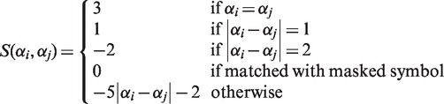It is sometimes helpful to mask parts of the sequence, for example, when the sequence has low-complexity regions or stretches with no measurement of genomic landscapes (e.g. centromere regions). We set the score to 0 when masked characters are aligned, because masked characters should not affect the obtained alignment. The score should be negative on average to prevent random sequences from being aligned (16). (We have also prepared a score matrix to detect waves with opposing oscillations. The score matrix for negative correlations is also set so the angles that differ the most will have the highest scores and gradually decrease as the angles become more acute.)

E-value calculation

The lastex application, included in the LAST software (16,17), calculates the likelihood of getting chance alignments (18) (the ‘E-value’) for a given score matrix and gap penalty. By employing an E-value threshold, we can filter out alignment pairs having low significance. In our analysis we set the E-value to 0.1.

RESULTS

Overview of the method

The general idea of our approach is to align genomic landscape data (collections of real-valued observations made at sequential positions along a chromosome) based on their topology. This will allow us to detect regions with similar shapes, which can lead to finding functionally interrelated regions. Our approach has five phases: (i) wavelet transformation, (ii) data reduction, (iii) symbolic representation, (iv) local alignment and (v) filtering (Figure 2). In this section, we will look at each step in detail.

Figure 2.

Overview of the proposed method to convert genomic landscape data into a series of symbols. (A) Raw data: an equally spaced landscape data set at the nominal scale (which is considered as a combination of multiple scales). (B) Wavelet transformation: the raw signal is transformed into a series of wavelet coefficients at a fixed wavelet scale. (C) Data reduction: PAA is used to lower the dimension of the data. (D) Extracting shape data: the angle to the adjacent PAA coefficient is calculated to retrieve the ‘shape’ of the landscape. (E) The process is then followed by assigning symbols according to the angles to obtain a set of sequences as an output. After converting the landscape data into sequences of symbols, sequence alignment is carried out to detect similar regions, which are reconverted into wavelet coefficients to select those waves with high correlation coefficients.

Wavelet transformation

The initial step of the procedure is to transform the landscape data into series of wavelet coefficients (Figure 2B). As explained in the introduction, genomic landscape data is usually the result of embedded and confounded biological processes working at different scales in the cell nucleus. Therefore, there could be a case where the data set is uncorrelated at short genomic ranges, but is strongly correlated at larger ranges (i.e. at longer wavelengths). To calculate the true correlation, we need to determine the correlation at relevant scales. Our solution to the problem is to utilize wavelet transformation to extract scale-specific information from independent and dependent variables and then detect scale-specific associations within the transformed data. Wavelet transformation (19) is a well-established mathematical procedure that is also used in bioinformatics (20) (see the ‘Materials and Methods’ section for details). Our work to apply wavelet transformation to genomic data was greatly inspired by the work of Thurman et al. (13), which was also used in the ENCODE project (2).

Data reduction

The bottleneck preventing the efficient search for similar regions in any genome-wide data set is the amount of data. We overcome this problem by using the data reduction technique called PAA, which is now widely used for time-series data (21). The data are divided into equally sized segments and the mean value of the data points falling within every segment is calculated (Figure 2C). The vector obtained from this process is a reduced representation of the original data, which enables handling large data sets such as genomic landscapes.

Symbolic representation

After we have reduced the original landscape data to a smaller number of data points, we convert the PAA coefficients into symbols. As we wish to detect those regions that have different amplitudes but similar shapes, we calculate the angle with respect to the adjacent PAA coefficient (see Figure 2D), and then convert angles to symbols (see the ‘Materials and Methods’ section for details).

This symbolic representation is inspired by a method called symbolic aggregate approximation (SAX), which is a procedure for converting time-series data into a series of symbols (22) and has been shown to be applicable to many analyses in data mining fields (http://www.cs.ucr.edu/~eamonn/SAX.htm). As a genomic landscape can also be considered a continuous data set along a certain interval (in this case, positions on a chromosome), we used SAX to transform the wavelet coefficients into a series of symbols.

Alignment of genomic landscapes

Treating a genomic landscape as a sequence of symbols allows us to incorporate alignment techniques that have been extensively studied in bioinformatics. We used the LAST alignment program, which finds similar regions between sequences (17). We chose LAST from other similar tools (e.g. BLAST, BLAT, BLASTZ) because (i) it allows a series of user-defined symbols and a score matrix to be set, (ii) it copes more efficiently with repetition-rich sequences (by employing variable length seeds) and (iii) it calculates whether the alignment is significant (by comparing the score with random sequences) and can be bounded by E-value (18). Sequence alignment returns local pairs of subsequences with high scores that are significant. Gaps are inserted between the symbols so that the score is maximized. Inserting gaps overcomes the problem of position distortion that prevents the detection of an accurate correlation between the local landscapes. We explain how to construct a score matrix in the ‘Materials and Methods’ section.

Filtering

To ensure the pairs are highly correlated, we took the original wavelet coefficients of the subsequences and calculated the Pearson correlation within each pair. Every data point with a gap (i.e. a data point that is aligned with a gap) was removed before the correlations were computed. The remaining pairs from this stage will be the final output of our procedure and represent a set of similar regions in genomic landscapes with high correlation coefficients. It is also possible to filter by the length of the alignment at this stage. Given an input of raw genomic landscape pairs, the above procedure returns aligned landscapes with high correlation coefficients. Examples are shown in Figure 3. The figures indicate that the landscapes are precisely aligned and that the overall topologies are highly similar.

Figure 3.

Examples of aligned genomic landscapes for H3K4me2 (blue line) and H3K9ac (green line). (A) H3K4me2 and H3K9ac are aligned precisely and have a high correlation coefficient (r = 0.94027). (B) Data are symbolized by using the angles between the data points, enabling alignment of landscapes with different absolute values but the same shape. (C) Our method is robust to position distortion because it can insert gaps to maximize the alignment score. (D) An example of alignment between highly variable (small scale) landscape data.

Assessment of proposed method

Overall assessment of the method is difficult as we have no pairs of data sets that are guaranteed to have or not to have a correlation. Therefore, in an attempt to estimate the performance, we used well-accepted pairs of data sets with known associations and checked whether the results of our procedure are consistent with previous findings.

Assessment using known ‘correlated’ landscapes

Di-methylated histone H3 at lysine 4 (H3K4me2) is known to be enriched at regions that have an active chromatin state, and acetylated histone H3 at lysine 9 (H3K9ac) is known to reduce the tightness of the chromatin state by changing the charge of the histone, resulting in an open chromatin region. These two histone modifications associated with active and open chromatin are known to be correlated (23,24). We tested whether the proposed method could correctly identify these similarities. Figure 3 shows part of the results produced. The overall topologies of the landscapes are precisely aligned with each other, showing very high correlation coefficients (r = 0.94 in Figure 3A). We also succeeded in aligning landscapes with different amplitudes but similar topologies (Figure 3B). Furthermore, we show that gaps can be inserted to cope with position distortion (Figure 3C). As a result, our method clearly showed that the landscapes of H3K4me2 and H3K9ac are positively correlated with each other genome-wide (Figure 1), which is consistent with the previous findings. This trend continued over all the scales examined (see column (a) in Table 1 and Figure 4) where the lines across diagonal show landscapes with a correlation coefficient higher than 0.7 at the exact position. Figure 3D is an example showing that H3K4me2 and H3K9ac exhibit a correlation even at smaller scales where the topology is more variable. The correlation between different histone landmarks has also been examined by Thurman et al. (25).

Table 1.

Diagonal coverage (%) as quantitative measurement of dot plots

Scale [Mbp]	(a) H3K4me2/ H3K9ac	(b) H3K4me2/ DNase I	(c) Gene Density/ LINE-1
1	98.98	96.28	5.10
0.50	99.36	95.39	2.71
0.25	99.61	90.82	2.02
0.10	99.25	86.08	0.00

Quantitative results of comparisons for (a) H3K4me2 (active) versus H3K9ac (open), (b) H3K4me2 versus DNase I and (c) gene density versus LINE-1 (L1) at multiple resolutions (scales). The column ‘Scale’ gives the scale of the wavelet transformation and the columns (a), (b) and (c) indicate the coverage of correlated regions in the diagonal area. The H3K4me2/H3K9ac and H3K4me2/DNase I pairs show high (within pair) similarity across the genome whereas the gene density/L1 pair barely shows any correlation. The values in the table are expressed as the mean for all chromosomes.

Figure 4.

Dot plot representation of two genomic landscapes, namely, H3K4me2 and H3K9ac, at multiple scales. H3K4me2 and H3K9ac show high coverage across the diagonals, indicating that they are exactly aligned. Note that all the aligned regions (indicated by red lines) in the figure have high correlations (greater than 0.7). See also Table 1 for quantitative results.

Landscapes from independent experiments

To investigate further the robustness of our method, we compared the landscapes from two independent experimental environments; data from active chromatin (H3K4me2) and chromatin accessibility (DNase I) were used. As chromatin is loosened during transcription, these two features are known to correlate with each other (2). Our method successfully detected a genome-wide correlation between these data (see column (b) in Table 1).

Assessment using known ‘uncorrelated’ landscapes

Next, we applied our method to well-known ‘uncorrelated’ landscape data. It has long been known that LINE-1 (L1) retrotransposons constitute one of the most successful families of retroelements in mammals and are abundant in gene-poor regions of the genome (26). We calculated the correlation between L1 and gene content to verify that our method does not mistakenly detect uncorrelated regions. Four different scales from coarse to fine were used. As opposed to the results from the H3K4me2/H3K9ac analysis, the pair did not show genome-wide correlation and showed no correlation at the exact position (see column (c) in Table 1 and Supplementary Figure S1). This result was consistent with what was expected from previous studies (7,26–29).

Processing time

The general aim of this work is to provide a genome-wide similarity search that will enable users to effectively explore the wealth of today's genomic landscape data. Therefore, processing time is an important factor. By utilizing a compact data representation and a well-studied sequence analysis technique, we have developed a method for comparing genomic landscapes at ultrahigh speed. For the H3K4me2/H3K9ac analysis at a single scale (with fixed parameters), the genome-wide intrachromosome similarity search is completed within 3–4 min and takes only about 15 min at four scales (Table 2). For more conservative run, with nine combinations of parameters merged (see ‘Materials and Methods’ section), it will take approximately 6–8 times more. This short processing time will allow systematic and comprehensive comparisons of many genomic landscapes and could be incorporated into the post-processing done immediately after downloading the data from a database such as the UCSC genome browser.

Table 2.

Processing time (in seconds) of each step at four scales

Scale [Mbp]	1	0.5	0.25	0.1	Total
Wavelet transformation	63.52	65.05	63.78	65.60	257.96
Symbol representation	22.97	25.07	25.21	26.86	100.12
Sequence alignment	57.85	55.33	54.48	63.73	231.38
Filtering	63.79	64.88	83.19	104.94	316.80
Total	208.14	210.34	226.66	261.13	906.26

The processing time was measured for intrachromosome comparison of histone modification data, H3K4me2 and H3K9ac, for chromosomes 1-22 and X. The number of symbols and the number of data points per symbol were set to 7 and 0.75 times the scale, respectively. We used a computer with a 2.67 GHz Intel Xeon Processor X5550, 24 GB of RAM and a Linux operating system.

Pipeline

Our pipeline is designed so various genomic features can be compared consecutively without any modification of the data. Users will only need to specify the data file and the path to it in the setting file. The information on which scale to investigate can also be fixed in this file, but unless the users have a prior knowledge about the scale, it is recommended to run the program at wide range of scales. Furthermore, our program supports parallel processing to speed up the calculations. The software implementation of our method is named ‘GeLATo’ which is an abbreviation for Genomic Landscape Alignment Tool.

Application to human genomic landscapes

The above benchmarks demonstrate that the method is capable of finding regions with similar landscape topologies, indicating that we can apply the method to other existing data. We conducted a comprehensive study of various human genomic landscapes and investigated the interrelations between the samples. A total of 13 samples available from the public database were selected, namely, ‘gene density’, ‘GC content’, ‘CTCF binding sites’, ‘conservation score (PhyloP)’, ‘Alu elements’, ‘LINE-1’, ‘replication timing (ES cell)’, ‘replication timing (NPC)’, ‘H3K4me2’, ‘H3K27me3’, ‘H3K9ac’, ‘DNase I’ and ‘DNA methylation (sperm)’. We then carried out all-to-all comparison for those landscapes at four separate scales, from fine to coarse, for a total of 312 comparisons using genome-wide data. To eliminate the effect of the parameter settings, such as number of symbols and data points used to represent a single symbol, we have internally merged all the results from different parameters. To interpret the results we used the diagonal coverage to assess the degree of correlation between two landscapes (Table 3 and Supplementary Table S2).

Table 3.

Comprehensive study of 13 genomic landscapes in human genome (scale: 1Mbp)

	Gene	GC	CTCF	Cons.	Alu	LINE	RT-ESC	RT-NPC	H3K4me2	H3K27me3	H3K9ac	DNaseI	DNAmeth.
Gene	–	48.39	68.42	4.59	93.80	5.10	83.45	65.28	91.00	14.35	77.86	82.09	5.19
GC	48.39	–	55.16	39.53	75.87	10.87	50.92	50.42	96.64	51.57	90.34	93.96	50.85
CTCF	68.42	55.16	–	0.00	39.46	0.00	46.52	40.23	77.29	36.61	50.69	87.43	0.67
Cons.	4.59	39.53	0.00	–	5.82	16.85	6.03	9.30	19.93	11.51	18.98	15.62	65.69
Alu	93.80	75.87	39.46	5.82	–	7.29	96.19	68.31	92.60	32.81	86.19	91.09	9.90
LINE	5.10	10.87	0.00	16.85	7.29	–	0.84	0.00	8.76	4.82	8.58	8.32	16.09
RT-ESC	83.45	50.92	46.52	6.03	96.19	0.84	–	93.78	94.85	22.00	84.65	81.18	4.73
RT-NPC	65.28	50.42	40.23	9.30	68.31	0.00	93.78	–	76.73	12.48	69.08	60.22	4.85
H3K4me2	91.00	96.64	77.29	19.93	92.60	8.76	94.85	76.73	–	81.80	98.98	96.28	17.69
H3K27me3	14.35	51.57	36.61	11.51	32.81	4.82	22.00	12.48	81.80	–	72.27	64.16	5.84
H3K9ac	77.86	90.34	50.69	18.98	86.19	8.58	84.65	69.08	98.98	72.27	–	85.38	21.28
DNaseI	82.09	93.96	87.43	15.62	91.09	8.32	81.18	60.22	96.28	64.16	85.38	–	17.69
DNAmeth.	5.19	50.85	0.67	65.69	9.90	16.09	4.73	4.85	17.69	5.84	21.28	17.69	–

The values listed in each column show the diagonal coverage, which is used as a measure of how well two landscapes are aligned at the exact position. DNAmeth.: DNA methylation; Cons.: Conservation. See Supplementary Table S2 for other scales.

Overall, correlation matrix values show higher correlation at a coarser scale, and the coverage gradually decreases as the scales become finer. For gene density, H3K4me2, which is an active chromatin landmark, shows high correlation of >90% with the diagonal coverage. The distribution of Alu elements and gene density also shows high coverage (93.80%), which indicates high similarity between them. This is consistent with the report that Alu elements are enriched in gene-rich regions (7). Furthermore, in order to check the reliability and significance of the diagonal coverage values, we calculated all the landscape pairs with one of the two samples in the reversed direction. If the diagonal coverage is due to a false positive, it is likely to also show up in pairs with opposite directions as they have the same complexity and composition of symbols. As a result, all pairs showed significantly low diagonal coverage at every scale studied, which indicates that diagonal coverage values are not caused by random effects (see Supplementary Table S3).

Genome-wide pattern of replication timing and the density of Alu elements are highly correlated

Replication timing is the temporal order of DNA replication at all coordinates in the genome (11,30,31). High (low) values indicate that the DNA segment is copied early (late) in interphase. On the other hand, Alu is the most abundant transposable element in human, comprising 11% of the total genomic DNA, and this element propagates by transposition to other regions within the genome. Alu elements are known to be distributed non-randomly along the human genome and have been proposed to be major players in shaping primate genomes (7,32).

We have found a striking similarity between these two intuitively unrelated landscapes (Figure 5). The degree of similarity are almost the same among chromosomes, showing nearly a 100% match (see Supplementary Figure S2). In average, the diagonal coverage at exact position in replication timing exceeded both of well acknowledged genomic features, GC contents and gene density, that has been known to show correlation with distribution of Alu elements from the early age of genome analysis (7) (see Table 3). Although Alu is one of the non-autonomous retrotransposons that require functional proteins encoded by long interspersed elements (LINEs) to mediate their retrotransposition (33), L1 does not show this similarity (see Table 3).

Figure 5.

Example of alignment results for the density of Alu elements and replication timing in ES cells (ESC). (A) Example of an aligned landscape at the 0.5 Mbp wavelet scale on human chromosome 4. (B) Dot plot representation of the two at the 1 Mbp scale on chromosome 16.

Replication timing of embryonic stem cells shows a high degree of correlation with Alu density at a wide range of scales

It is known that the replication timing program changes during development (11). Interestingly, Figure 6 clearly shows that Alu density more strongly correlates with replication timing in embryonic stem (ES) cells than in neural precursor cells (NPCs): the coverage percentage along the diagonal of a dot plot is higher for ES cells at every scale examined. We suspect that this is because only mutations in germline cells are passed onto the next generation. In addition, to understand how the scale size affects the degree of diagonal coverage for these pairs, the diagonal coverage was calculated at 15 different scales (Figure 7), along with GC content and gene density. As shown in Figure 7, replication timing (in ES cells) shows the highest coverage for a wide range of scales among the three samples. The most distinctive feature is that unlike GC content and gene density where the coverage gradually decreases as the scale becomes smaller, the coverage for replication timing is high and stationary until 0.25–0.3 Mbp, where it shows a sudden drop. Considering that false-negative coverage is kept within 5–6% (see Supplementary Figure S6), the result is most likely related to an attribute of replication timing. The observation that the diagonal coverage becomes relatively low at a small scale agrees with the report that DNA replication is regulated at the level of large chromosomal domains, 0.5–5 Mb in size (34).

Figure 6.

Averaged diagonal coverage of the dot plot over all chromosomes: Alu density versus replication timing (RT) for ES cells (black bar) and Alu density versus RT for NPCs (gray bar). ES cells show a higher diagonal coverage in the dot plot than NPCs at all scales examined.

Figure 7.

Transition of the diagonal coverage between density of Alu elements and three different landscapes (RT, replication timing; GC, GC content; Gene, gene density) over 15 different scales.

Degree of similarity coverage changes with repeat types

We further investigated the relationship between replication timing and the distribution patterns of various repeat elements in the human genome, including repeats from SINE and LINE (Table 4). The results show that only Alu elements have a high degree of diagonal coverage against replication timing, almost no coverage against L1 and L2 in the LINE family and very low coverage against MIR from the SINE family. The most interesting finding was that Alu subfamilies of different genetic age showed different degrees of coverage: the oldest, AluJ (active 65–40 million years ago, mya), had the highest coverage, followed by AluS (45–25 mya) and the least similar in the youngest Alu, AluY (30 mya to present) (7,35). Furthermore, the coverage was especially high for replication timing in ES cells and iPS cells but not as high in NPCs and lymphoblastoid cells.

Table 4.

Correlations between replication timing and density of various repeat elements (scale: 1Mbp)

		RT					SINE					LINE
		ESC	ESC2	iPS	NPC	Lympho.	Alu	AluJ	AluS	AluY	MIR	L1	L2
RT	ESC	–	99.00	98.88	93.78	81.04	96.19	95.99	92.62	53.90	9.42	0.00	5.86
	ESC2	99.00	–	98.48	96.36	87.11	91.18	96.02	91.79	58.82	7.26	0.00	5.45
	iPS	98.88	98.48	–	90.64	75.32	94.66	93.97	93.40	59.54	7.91	0.00	4.63
	NPC	93.78	96.36	90.64	–	70.29	68.31	69.88	66.91	14.90	12.52	0.00	10.06
	Lympho	81.04	87.11	75.32	70.29	–	71.13	74.82	71.27	32.09	7.97	0.91	3.72
SINE	Alu	96.19	91.18	94.66	68.31	71.13	–	98.76	98.97	96.34	19.86	5.90	19.23
	AluJ	95.99	96.02	93.97	69.88	74.82	98.76	–	98.43	89.23	20.22	2.40	20.62
	AluS	92.62	91.79	93.40	66.91	71.27	98.97	98.43	–	96.10	21.44	5.90	11.57
	AluY	53.90	58.82	59.54	14.90	32.09	96.34	89.23	96.10	–	3.81	7.28	6.93
	MIR	9.42	7.26	7.91	12.52	7.97	19.86	20.22	21.44	3.81	–	1.30	96.47
LINE	L1	0.00	0.00	0.00	0.00	0.91	5.90	2.40	5.90	7.28	1.30	–	3.41
	L2	5.86	5.45	4.63	10.06	3.72	19.23	20.62	11.57	6.93	96.47	3.41	–

RT, replication timing; Lympho, Lymphoblastoid. See Supplementary Table S4 for other scales.

Relation of repeat elements and replication timing in mouse genome

Next, to check whether correlation can also be found in other species, we conducted a comprehensive study using various repeats and replication timing data in the mouse genome. Although copies of Alu elements in human and mouse have amplified and duplicated independently in the two genomes (7,36), we found high diagonal coverage between Alu and replication timing in the mouse genome, similarly (see Supplementary Table S5). In contrast to SINE repeats in human where only one dominant type of repeat (Alu element) succeeded in its expansion, the SINE family in mouse have several types of repeats (e.g. Alu, B2 and B4) (7). To test whether the correlation is specific to Alu elements, we furthermore carried out alignments of other repeat elements. As a result, B2 and B4 from the SINE family also showed high diagonal coverage against replication timing (see Supplementary Table S5) and the trends in coverage according to scale were highly similar (see Figure 7 and Supplementary Figure S7). In both human and mouse, MIR showed almost no correlation.

Finding correlated regions at different positions

So far we have shown that the pipeline is useful for detecting those pairs that show high correlation at exact positions for data on various landscapes. To exhibit the strength of the proposed method where similar landscape topologies in different positions can also be retrieved, we explored this case by using artificial data created with the H3K4me2 landscape in human chromosome 1. Although the data are relatively simple, we verified that this approach can align all the regions of the shuffled data (see Supplementary Figure S4) and can detect all the embedded motifs (see Supplementary Figure S5).

Comparative genomic landscape

To further demonstrate, using real data, that our framework can also compare landscapes from different species, alignment of DNA methylation landscapes in human and chimpanzee was carried out. The major difference in human and chimpanzee is that human chromosome 2 is derived from two smaller chromosomes from chimpanzee (chromosome 2A and 2B) and they have fused to create chromosome 2 (37). Therefore, in the chimpanzee genome, the coordinates are different from those in human. We have confirmed that the landscape of DNA methylation is conserved between the human and chimpanzee genomes by using genome-wide data on DNA methylation measured in sperm. This is consistent with the results of the original work (12) (Figure 8).

Figure 8.

Alignment of DNA methylation landscapes between human and chimpanzee. Human chromosome 2 is a product of fusion of ancestral chimpanzee chromosomes 2A and 2B. Although the positions and chromosomes are different, the results show that the landscapes of DNA methylation in both chimpanzee chromosomes 2A (A) and 2B (B) are precisely aligned with human chromosome 2. This finding is consistent with early studies.

Taken together, we show that our pipeline can be applied to detect pairs of correlated regions at different genomic positions.

DISCUSSION

We developed a method that can compare different types of landscapes and obtain pairs of local regions that have similar topologies. We demonstrated that this approach is effective for the purpose of comparing landscape topologies (Figure 3) and offers several advantages: fast processing speed (Table 2), the ability to handle genome-wide data sets and an architecture that allows seamless comparison of multiple samples (Table 3).

Our challenge was to incorporate the concept of scale from the field of landscape ecology into the analysis of genomic landscapes as genomes are regulated at different scales, from macroscopic to mesoscopic to microscopic. For instance, levels of regulation include nucleosomes, chromatin loops, matrix attachment regions (38), nuclear lamina and chromosome territories (5,14,39–41).

There are many cases in genomic landscapes where DNA sequences are the same but the DNA is modified (e.g. histone modification, DNA methylation, nucleosome positioning and other chip-sequencing data in different cell line or tissues). This will provide a rough determination of which existing landscape data are associated with the new data (Table 3) that cannot be accomplished through the alignment of DNA sequences. For genomic landscape data, one could use the developed platform to compare genomic landscapes across species (‘comparative genomic landscapes’) and to study how a particular landscape has evolved over time (Figure 8).

In the future, it will also be interesting to search for ‘landscape motifs’ where the corresponding DNA sequences are not similar but their landscape topologies are. Although we have checked that all the artificially embedded motifs appear on corresponding regions of the dot plot (see Supplementary Figure S5) and some examples are detected as self-similar regions (see Supplementary Figure S3), the pipeline needs to be extended so that it can group all the similar regions and obtain distinctive shapes for real biological data, as currently, the retrieval of similar regions is limited to pairs. We, therefore, intend to extend our approach to multiple alignment. The idea is to compute the local alignments for every pair of sequences as described in this article, then cluster such alignments into blocks of approximately globally alignable subsequences, determine block boundaries and, finally, multiply align these blocks (42).

Comparison with existing methods

Dynamic time warping (DTW) (43) is another technique that has long been used to compare time-series data. (DTW is similar to the Smith–Waterman algorithm (44) in sequence alignment.) However, a straightforward implementation of DTW has a time and space complexity of O(n²) (where n is the length of the data), which is unsuitable for our case because new genome-wide data are constantly flowing in at a prodigious rate. We need to have an efficient approach that copes with the high dimensionality of genome data. Our approach succeeded in accomplishing this by converting the landscape data into symbols and using well-known sequence alignment techniques.

As explained earlier, there are only a few works that focus on the interrelations of genomic landscapes. The pioneers in analyzing continuous functional genomic data are Thurman et al. (2,13,45). A distinction between their approach and ours is that our approach ‘aligns’ genomic landscapes by conducting extensive searches for similar topologies over all coordinates. This can be used to search for motifs or to compare different species and is not limited to a fixed position. In addition, gaps can be inserted to cope with position distortion, a procedure that could be adjusted to suit experimental conditions.

Correlation between replication timing and distribution of Alu elements: possible scenarios

The landscape of the replication timing showed high correlation to the landscape of Alu density over the entire human genome (Table 3). The common feature among the two landscapes is that they are both associated with the structure of chromatin. For Alu elements, they occupy ∼11% of the human genome and have had a substantial impact on shaping our genome over the years of evolution (7,28,29,46). On the other hand, recent studies have also revealed that replication timing is related to the 3D organization of chromosomes in the cell nucleus and that a transition in the timing is facilitated by chromatin change (11,28,30) at the level of large chromosomal domains, 0.5–5 Mbp in size (34). The correlation between the two is high and stationary up to the 0.25–0.3 Mbp scale, where it shows a sudden drop, in human (Figure 7) and mouse (see Supplementary Figure S7), pointing to the possibility that chromatin structure is associated with the correlation between the two. Here, we discuss two possible scenarios that could explain why the two landscapes show high similarity.

The first scenario is straightforward and considers ‘structure-biased insertions’; Alu elements transpose to those regions with early replication timing. Since replication timing and Hi-C data are closely correlated (11), this, in other words, indicates that insertions are made at highly accessible regions of chromatin structure. As free diffusion is known to be the main mode of transport in living cells (47), including diffusive movement of proteins, lipids and nucleic acids (5), Alu elements are also likely to diffuse in the cell nucleus. Thus, there is a greater chance of Alu elements inserting at open chromatin region leading to close similarity between landscapes of replication timing and Alu elements. The high diagonal coverage between Alu elements and DNase I, which is often used as a measure of chromatin accessibility, also supports this view (Table 3). Although this hypothesis seems to account for the correlation well, the scenario cannot explain the results of a detailed study that uses different subfamilies of Alu elements (Table 4). According to the result, recently transposed AluY does not show coverage as high as the older AluS and AluJ. Because replication timing reflects the current structure of the nucleus, younger Alu would reflect that structure to a greater extent than would the older insertions.

The second scenario addresses this point, and considers ‘structure-biased selection’ of Alu elements. Although it is well known that Alu elements are observed in GC-rich regions, originally, both Alu and LINE-1 (L1) elements integrate into similar AT-rich regions as Alu uses the reverse transcriptase from L1. In contrast to L1, Alu elements seem to shift toward GC-rich DNA over time (29,48). Our hypothesis considers that the selection difference after Alu insertion events is influenced by the chromatin structure, thus leading to the similarity between the landscapes of Alu elements and replication timing. The connection between chromatin structure and mutation rates has previously been studied; it is the lowest in open regions and the highest in a closed chromatin structure (49) that supports our view. This is explained by the increasing DNA methylation level that reflects a negative correlation between timing and gene expression (50), which is directly linked to the status of chromatin loops. This is consistent with the observation that mutation rate is markedly increased in later-replicating regions of the human genome (51), which is also found in other species (52). Moreover, in the study of insertion distribution, the evolutionarily young Alu (AluY) insertions were found to be distributed relatively evenly in both the chimpanzee and human chromosomes (53). This supports the hypothesis that the selection, after the insertion, shapes the current observed distribution, suggesting that recently transposed AluY is still in the process of being eliminated by selection.

It is still an open question as to why this is limited to Alu (or to active SINE elements in mouse) and not L1 (Table 4), which uses the same mechanisms as transpose. There are numerous studies that have focused on factors that distinguish L1 from Alu elements (27,54,55). One interesting study by Kroutter et al. (56), shows that Alu RNAs can retrotranspose rapidly, whereas L1 RNAs take almost 24 h longer, which is caused by the way cells manage pol III and pol II (mRNA) transcripts affecting the timing of a transcript going through the retrotransposition pathway.

CONCLUSION

We have developed an ultrafast method for comparing genome-wide data on genomic landscapes. To our knowledge, this is the first method to align the landscapes according to their topology at multiple resolutions. Our approach is robust to position distortion and copes with the high dimensionality of genomic data. The information discovered through our approach should facilitate further exploration of genomic landscapes and how they affect each other within a living cell nucleus. Our pipeline GeLATo is freely available from http://www.cb.k.u-tokyo.ac.jp/asailab/gelato.

SUPPLEMENTARY DATA

Supplementary Data are available at NAR Online: Supplementary Tables 1–5 and Supplementary Figures 1–7.

FUNDING

Grant-in-Aid for Scientific Research on Innovative Areas; the Global Center of Excellence program ‘Deciphering Biosphere from Genome Big Bang’. Funding for open access charge: Grant-in-Aid for Scientific Research on Innovative Areas.

Conflict of interest statement. None declared.

REFERENCES

- 1.Raney BJ, Cline MS, Rosenbloom KR, Dreszer TR, Learned K, Barber GP, Meyer LR, Sloan CA, Malladi VS, Roskin KM, et al. ENCODE whole-genome data in the UCSC genome browser (2011 update) Nucleic Acids Res. 2011;39:D871–D875. doi: 10.1093/nar/gkq1017. [DOI] [PMC free article] [PubMed] [Google Scholar]
- 2.ENCODE Consortium (2007) Identification and analysis of functional elements in 1 human genome by the ENCODE pilot project. Nature. 447:799–816. doi: 10.1038/nature05874. [DOI] [PMC free article] [PubMed] [Google Scholar]
- 3.Kent WJ, Sugnet CW, Furey TS, Roskin KM, Pringle TH, Zahler AM, Haussler D. The human genome browser at UCSC. Genome Res. 2002;12:996–1006. doi: 10.1101/gr.229102. [DOI] [PMC free article] [PubMed] [Google Scholar]
- 4.Fujita PA, Rhead B, Zweig AS, Hinrichs AS, Karolchik D, Cline MS, Goldman M, Barber GP, Clawson H, Coelho A, et al. The UCSC Genome Browser database: update 2011. Nucleic Acids Res. 2011;39:D876–D882. doi: 10.1093/nar/gkq963. [DOI] [PMC free article] [PubMed] [Google Scholar]
- 5.Misteli T. Beyond the sequence: cellular organization of genome function. Cell. 2007;128:787–800. doi: 10.1016/j.cell.2007.01.028. [DOI] [PubMed] [Google Scholar]
- 6.Filatov LV, Mamayeva SE, Tomilin NV. Non-random distribution of Alu-family repeats in human chromosomes. Mol. Biol. Rep. 1987;12:117–122. doi: 10.1007/BF00368879. [DOI] [PubMed] [Google Scholar]
- 7.Batzer MA, Deininger PL. Alu repeats and human genomic diversity. Nat. Rev. Genet. 2002;3:370–379. doi: 10.1038/nrg798. [DOI] [PubMed] [Google Scholar]
- 8.Kvikstad EM, Makova KD. The (r)evolution of SINE versus LINE distributions in primate genomes: sex chromosomes are important. Genome Res. 2010;20:600–613. doi: 10.1101/gr.099044.109. [DOI] [PMC free article] [PubMed] [Google Scholar]
- 9.Grover D, Mukerji M, Bhatnagar P, Kannan K, Brahmachari SK. Alu repeat analysis in the complete human genome: trends and variations with respect to genomic composition. Bioinformatics. 2004;20:813–817. doi: 10.1093/bioinformatics/bth005. [DOI] [PubMed] [Google Scholar]
- 10.Turner M, Gardner RH, O'Neill RV. Landscape Ecology in Theory and Practice: Pattern and Process. New York, USA: Springer; 2001. [Google Scholar]
- 11.Ryba T, Hiratani I, Lu J, Itoh M, Kulik M, Zhang J, Schulz TC, Robins AJ, Dalton S, Gilbert DM. Evolutionarily conserved replication timing profiles predict long-range chromatin interactions and distinguish closely related cell types. Genome Res. 2010;20:761–770. doi: 10.1101/gr.099655.109. [DOI] [PMC free article] [PubMed] [Google Scholar]
- 12.Molaro A, Hodges E, Fang F, Song Q, McCombie WR, Hannon GJ, Smith AD. Sperm methylation profiles reveal features of epigenetic inheritance and evolution in primates. Cell. 2011;146:1029–1041. doi: 10.1016/j.cell.2011.08.016. [DOI] [PMC free article] [PubMed] [Google Scholar]
- 13.Thurman RE, Noble WS, Stamatoyannopoulos JA. Multi-scale correlations in continuous genomic data. Pac. Symp. Biocomput. 2008:201–215. doi: 10.1142/9789812776136_0021. [DOI] [PubMed] [Google Scholar]
- 14.Woodcock CL, Ghosh RP. Chromatin higher-order structure and dynamics. Cold Spring Harb. Perspect. Biol. 2010;2:a000596. doi: 10.1101/cshperspect.a000596. [DOI] [PMC free article] [PubMed] [Google Scholar]
- 15.Cremer T, Cremer M, Dietzel S, Muller S, Solovei I, Fakan S. Chromosome territories–a functional nuclear landscape. Curr. Opin. Cell Biol. 2006;18:307–316. doi: 10.1016/j.ceb.2006.04.007. [DOI] [PubMed] [Google Scholar]
- 16.Frith MC, Hamada M, Horton P. Parameters for accurate genome alignment. BMC Bioinformatics. 2010;11:80. doi: 10.1186/1471-2105-11-80. [DOI] [PMC free article] [PubMed] [Google Scholar]
- 17.Kielbasa SM, Wan R, Sato K, Horton P, Frith MC. Adaptive seeds tame genomic sequence comparison. Genome Res. 2011;21:487–493. doi: 10.1101/gr.113985.110. [DOI] [PMC free article] [PubMed] [Google Scholar]
- 18.Sheetlin S, Park Y, Spouge JL. The Gumbel pre-factor k for gapped local alignment can be estimated from simulations of global alignment. Nucleic Acids Res. 2005;33:4987–4994. doi: 10.1093/nar/gki800. [DOI] [PMC free article] [PubMed] [Google Scholar]
- 19.Percival DB, Walden AT. Wavelet Methods for Time Series Analysis (Cambridge Series in Statistical and Probabilistic Mathematics) UK: Cambridge University Press; 2000. [Google Scholar]
- 20.Lio P. Wavelets in bioinformatics and computational biology: state of art and perspectives. Bioinformatics. 2003;19:2–9. doi: 10.1093/bioinformatics/19.1.2. [DOI] [PubMed] [Google Scholar]
- 21.Keogh E, Chakrabarti K, Pazzani M, Mehrotra S. Dimensionality reduction for fast similarity search in large time series databases. Knowl. Info. Syst. 2001;3:263–286. [Google Scholar]
- 22.Wei L, Lin J, Keogh E, Lonardi S. Experiencing SAX: a novel symbolic representation of time series. Data Min. Knowl. Discov. 2007;15:107–144. [Google Scholar]
- 23.van Leeuwen F, van Steensel B. Histone modifications: from genome-wide maps to functional insights. Genome Biol. 2005;6:113. doi: 10.1186/gb-2005-6-6-113. [DOI] [PMC free article] [PubMed] [Google Scholar]
- 24.Wang Z, Zang C, Rosenfeld JA, Schones DE, Barski A, Cuddapah S, Cui K, Roh TY, Peng W, Zhang MQ, et al. Combinatorial patterns of histone acetylations and methylations in the human genome. Nat. Genet. 2008;40:897–903. doi: 10.1038/ng.154. [DOI] [PMC free article] [PubMed] [Google Scholar]
- 25.Young MD, Willson TA, Wakefield MJ, Trounson E, Hilton DJ, Blewitt ME, Oshlack A, Majewski IJ. ChIP-seq analysis reveals distinct H3K27me3 profiles that correlate with transcriptional activity. Nucleic Acids Res. 2011;39:7415–7427. doi: 10.1093/nar/gkr416. [DOI] [PMC free article] [PubMed] [Google Scholar]
- 26.Graham T, Boissinot S. The genomic distribution of L1 elements: the role of insertion bias and natural selection. J. Biomed. Biotechnol. 2006;2006:75327. doi: 10.1155/JBB/2006/75327. [DOI] [PMC free article] [PubMed] [Google Scholar]
- 27.Deininger P. Alu elements: know the SINEs. Genome Biol. 2011;12:236. doi: 10.1186/gb-2011-12-12-236. [DOI] [PMC free article] [PubMed] [Google Scholar]
- 28.Jurka J. Evolutionary impact of human Alu repetitive elements. Curr. Opin. Genet. Dev. 2004;14:603–608. doi: 10.1016/j.gde.2004.08.008. [DOI] [PubMed] [Google Scholar]
- 29.Lander ES, Linton LM, Birren B, Nusbaum C, Zody MC, Baldwin J, Devon K, Dewar K, Doyle M, FitzHugh W, et al. Initial sequencing and analysis of the human genome. Nature. 2001;409:860–921. doi: 10.1038/35057062. [DOI] [PubMed] [Google Scholar]
- 30.Guillou E, Ibarra A, Coulon V, Casado-Vela J, Rico D, Casal I, Schwob E, Losada A, Mendez J. Cohesin organizes chromatin loops at DNA replication factories. Genes Dev. 2010;24:2812–2822. doi: 10.1101/gad.608210. [DOI] [PMC free article] [PubMed] [Google Scholar]
- 31.Berbenetz NM, Nislow C, Brown GW. Diversity of eukaryotic DNA replication origins revealed by genome-wide analysis of chromatin structure. PLoS Genet. 2010;6:e1001092. doi: 10.1371/journal.pgen.1001092. [DOI] [PMC free article] [PubMed] [Google Scholar]
- 32.Urrutia AO, Ocana LB, Hurst LD. Do Alu repeats drive the evolution of the primate transcriptome? Genome Biol. 2008;9:R25. doi: 10.1186/gb-2008-9-2-r25. [DOI] [PMC free article] [PubMed] [Google Scholar]
- 33.Levin HL, Moran JV. Dynamic interactions between transposable elements and their hosts. Nat. Rev. Genet. 2011;12:615–627. doi: 10.1038/nrg3030. [DOI] [PMC free article] [PubMed] [Google Scholar]
- 34.Weddington N, Stuy A, Hiratani I, Ryba T, Yokochi T, Gilbert DM. ReplicationDomain: a visualization tool and comparative database for genome-wide replication timing data. BMC Bioinformatics. 2008;9:530. doi: 10.1186/1471-2105-9-530. [DOI] [PMC free article] [PubMed] [Google Scholar]
- 35.Price AL, Eskin E, Pevzner PA. Whole-genome analysis of Alu repeat elements reveals complex evolutionary history. Genome Res. 2004;14:2245–2252. doi: 10.1101/gr.2693004. [DOI] [PMC free article] [PubMed] [Google Scholar]
- 36.Tsirigos A, Rigoutsos I. Alu and b1 repeats have been selectively retained in the upstream and intronic regions of genes of specific functional classes. PLoS Comput. Biol. 2009;5:e1000610. doi: 10.1371/journal.pcbi.1000610. [DOI] [PMC free article] [PubMed] [Google Scholar]
- 37. The Chimpanzee Sequencing and Analysis Consortium. (2005) Initial sequence of the chimpanzee genome and comparison with the human genom E. Nature, 437, 69–87. [DOI] [PubMed]
- 38.Ottaviani D, Lever E, Takousis P, Sheer D. Anchoring the genome. Genome Biol. 2008;9:201. doi: 10.1186/gb-2008-9-1-201. [DOI] [PMC free article] [PubMed] [Google Scholar]
- 39.Kind J, van Steensel B. Genome-nuclear lamina interactions and gene regulation. Curr. Opin. Cell Biol. 2010;22:320–325. doi: 10.1016/j.ceb.2010.04.002. [DOI] [PubMed] [Google Scholar]
- 40.Cremer T, Cremer M. Chromosome territories. Cold Spring Harb. Perspect. Biol. 2010;2:a003889. doi: 10.1101/cshperspect.a003889. [DOI] [PMC free article] [PubMed] [Google Scholar]
- 41.Lieberman-Aiden E, van Berkum NL, Williams L, Imakaev M, Ragoczy T, Telling A, Amit I, Lajoie BR, Sabo PJ, Dorschner MO, et al. Comprehensive mapping of long-range interactions reveals folding principles of the human genome. Science. 2009;326:289–293. doi: 10.1126/science.1181369. [DOI] [PMC free article] [PubMed] [Google Scholar]
- 42.Phuong TM, Do CB, Edgar RC, Batzoglou S. Multiple alignment of protein sequences with repeats and rearrangements. Nucleic Acids Res. 2006;34:5932–5942. doi: 10.1093/nar/gkl511. [DOI] [PMC free article] [PubMed] [Google Scholar]
- 43.Sakoe H, Chiba S. Dynamic programming algorithm optimization for spoken word recognition. IEEE. Acoust. Speech. 1978;26:43–49. [Google Scholar]
- 44.Smith TF, Waterman MS. Identification of common molecular subsequences. J. Mol. Biol. 1981;147:195–197. doi: 10.1016/0022-2836(81)90087-5. [DOI] [PubMed] [Google Scholar]
- 45.Thurman RE, Day N, Noble WS, Stamatoyannopoulos JA. Identification of higher-order functional domains in the human ENCODE regions. Genome Res. 2007;17:917–927. doi: 10.1101/gr.6081407. [DOI] [PMC free article] [PubMed] [Google Scholar]
- 46.Hedges DJ, Batzer MA. From the margins of the genome: mobile elements shape primate evolution. Bioessays. 2005;27:785–794. doi: 10.1002/bies.20268. [DOI] [PubMed] [Google Scholar]
- 47.Vaz WL. Diffusion and chemical reactions in phase-separated membranes. Biophys. Chem. 1994;50:139–145. doi: 10.1016/0301-4622(94)85026-7. [DOI] [PubMed] [Google Scholar]
- 48.Hackenberg M, Bernaola-Galvan P, Carpena P, Oliver JL. The biased distribution of Alus in human isochores might be driven by recombination. J. Mol. Evol. 2005;60:365–377. doi: 10.1007/s00239-004-0197-2. [DOI] [PubMed] [Google Scholar]
- 49.Prendergast JG, Campbell H, Gilbert N, Dunlop MG, Bickmore WA, Semple CA. Chromatin structure and evolution in the human genome. BMC Evol. Biol. 2007;7:72. doi: 10.1186/1471-2148-7-72. [DOI] [PMC free article] [PubMed] [Google Scholar]
- 50.Chen CL, Rappailles A, Duquenne L, Huvet M, Guilbaud G, Farinelli L, Audit B, d'Aubenton Carafa Y, Arneodo A, Hyrien, et al. Impact of replication timing on non-CpG and CpG substitution rates in mammalian genomes. Genome Res. 2010;20:447–457. doi: 10.1101/gr.098947.109. [DOI] [PMC free article] [PubMed] [Google Scholar]
- 51.Stamatoyannopoulos JA, Adzhubei I, Thurman RE, Kryukov GV, Mirkin SM, Sunyaev SR. Human mutation rate associated with DNA replication timing. Nat. Genet. 2009;41:393–395. doi: 10.1038/ng.363. [DOI] [PMC free article] [PubMed] [Google Scholar]
- 52.Agier N, Fischer G. The mutational profile of the yeast genome is shaped by replication. Mol. Biol. Evol. 2012;29:905–913. doi: 10.1093/molbev/msr280. [DOI] [PubMed] [Google Scholar]
- 53.Hedges DJ, Callinan PA, Cordaux R, Xing J, Barnes E, Batzer MA. Differential alu mobilization and polymorphism among the human and chimpanzee lineages. Genome Res. 2004;14:1068–1075. doi: 10.1101/gr.2530404. [DOI] [PMC free article] [PubMed] [Google Scholar]
- 54.Lovsin N, Peterlin BM. APOBEC3 proteins inhibit LINE-1 retrotransposition in the absence of ORF1p binding. Ann. N. Y. Acad. Sci. 2009;1178:268–275. doi: 10.1111/j.1749-6632.2009.05006.x. [DOI] [PMC free article] [PubMed] [Google Scholar]
- 55.Schumann GG. APOBEC3 proteins: major players in intracellular defence against LINE-1-mediated retrotransposition. Biochem. Soc. Trans. 2007;35:637–642. doi: 10.1042/BST0350637. [DOI] [PubMed] [Google Scholar]
- 56.Kroutter EN, Belancio VP, Wagstaff BJ, Roy-Engel AM. The RNA polymerase dictates ORF1 requirement and timing of LINE and SINE retrotransposition. PLoS Genet. 2009;5:e1000458. doi: 10.1371/journal.pgen.1000458. [DOI] [PMC free article] [PubMed] [Google Scholar]
Associated Data
This section collects any data citations, data availability statements, or supplementary materials included in this article.