Genomic dark matter: the reliability of short read mapping illustrated by the genome mappability score

Abstract

Motivation: Genome resequencing and short read mapping are two of the primary tools of genomics and are used for many important applications. The current state-of-the-art in mapping uses the quality values and mapping quality scores to evaluate the reliability of the mapping. These attributes, however, are assigned to individual reads and do not directly measure the problematic repeats across the genome. Here, we present the Genome Mappability Score (GMS) as a novel measure of the complexity of resequencing a genome. The GMS is a weighted probability that any read could be unambiguously mapped to a given position and thus measures the overall composition of the genome itself.

Results: We have developed the Genome Mappability Analyzer to compute the GMS of every position in a genome. It leverages the parallelism of cloud computing to analyze large genomes, and enabled us to identify the 5–14% of the human, mouse, fly and yeast genomes that are difficult to analyze with short reads. We examined the accuracy of the widely used BWA/SAMtools polymorphism discovery pipeline in the context of the GMS, and found discovery errors are dominated by false negatives, especially in regions with poor GMS. These errors are fundamental to the mapping process and cannot be overcome by increasing coverage. As such, the GMS should be considered in every resequencing project to pinpoint the ‘dark matter’ of the genome, including of known clinically relevant variations in these regions.

Availability: The source code and profiles of several model organisms are available at http://gma-bio.sourceforge.net

Contact: hlee@cshl.edu

Supplementary Information: Supplementary data are available at Bioinformatics online.

1 INTRODUCTION

1.1 Background

DNA sequencing technology has dramatically improved in the past decade so that today an individual human genome can be sequenced for less than $10 000 and in less than 2 weeks (Drmanac et al., 2010), compared to years of effort and hundreds of millions of dollars for the first sequenced human genome (Stein, 2010). This dramatic improvement has lead to an exponential growth in sequencing, including several large projects to sequence thousands of human genomes and exomes, such as the (1000 Genomes Project Consortium, 2010) or (International Cancer Genome Consortium, 2010). Other projects, such as (ENCODE Project Consortium, 2004) and (modENCODE Consortium, 2010), are extensively using resequencing and read mapping to discover novel genes and binding sites.

The output of current DNA sequencing instruments consists of billions of short, 25–200 bp sequences of DNA called reads, with an overall per base error rate around 1–2% (Bentley et al., 2008). In the case of whole genome resequencing, these short reads will originate from random locations in the genome, but nevertheless, entire genomes can be accurately studied by oversampling the genome, and then aligning or ‘mapping’ each read to the reference genome to computationally identify where it originated. Once the entire collection of reads has been mapped, variations in the sample can be identified by the pileup of reads that significantly disagree from the reference genome (Fig. 1).

Fig. 1.

The top sequence represents the reference genome, with many individual reads mapped to the sequence beneath. The left highlighted column illustrates a homozygous substitution and the right highlighted column illustrates a heterozygous substitution. Two green reads are same sequence, which means the read can be mapped to multiple position. Consequently the origination is ambiguous

The leading short read mapping algorithms, including BWA (Li and Durbin, 2009), Bowtie (Langmead et al., 2009), and SOAP (Li et al., 2009b), all try to identify the best mapping position for each read that minimizes the number of differences between the read and the genome, i.e. the edit distance of the nucleotide strings, possibly weighted by base quality value. This is made practical through sophisticated indexing schemes, such as the Burrows–Wheeler transform (Burrows and Wheeler, 1994), so that many billions of reads can be efficiently mapped allowing for both sequencing errors and true variations. The primary complication of short read mapping is that a read may map equally well or nearly equally well to multiple positions because of repetitive sequences in the genome. Notably, nearly 50% of the human genome consists of repetitive elements, including certain repeats that occur thousands of times throughout (International Human Genome Sequencing Consortium, 2001).

For resequencing projects, the fraction of repetitive content depends on read length and allowed error rate. At one extreme, all single base reads would be repetitive, while chromosome length reads would not be repetitive at all. Similarly, increasing the allowed error rate increases the fraction of the genome that is repetitive. The short read mapping algorithms use edit distance and other read characteristics to compute a mapping quality score for each mapped read (Li et al., 2008). The mapping quality score estimates the probability that the assigned location is the correct position given the edit-distance of the alignment relative to the edit-distance of alternate alignments. This metric advanced the state-of-the-art for resequencing studies because then the variation discovery algorithms and other post-mapping algorithms could use this score to rule out false-positive variations caused by incorrectly mapped reads. However, as we show below, this metric is very sensitive to small changes in read positions or read qualities. Furthermore, it does not measure the ‘mappability’ of the genome itself to show where reads can be confidently mapped, only the confidence of individual reads that have already been mapped. There have been a few attemps to define mappability, focusing on the uniqueness of fixed length kmers (http://genomebrowser.wustl.edu/cgi-bin/hgTrackUi?db=hg18&g=wgEncodeMapability) or uniqueness of kmers allowing a small number of differences (Koehler et al., 2010). However, these metrics do not fully capture all of the experimental conditions of a sequencing experiment, such as read length, error rate, error type or library characteristics.

Addressing these limitations, we have developed the Genome Mappability Analyzer (GMA) pipeline that leverages the mapping quality score and other metrics into a new probabilistic metric called the Genome Mappability Score (GMS). The GMS measures the inherent uncertainty of mapping reads to each position in the genome as a weighted probability of mapping certainty. We have applied the GMA to compute the GMS profile for several important genomes under a variety of experimental parameters to measure the relative effect in mappability with respect to read length, error rate and sample preparation. In further experiments, we relate the GMS profile to the accuracy of the widely used BWA/SAMtools single nucleotide polymorphism (SNP) discovery algorithm. Our experiments show that, even at very high coverage of the genome, most variation discovery errors are false negatives and most of these errors occur in regions with low GMS values. Furthermore, virtually all mutations reported by the 1000 Genomes project (1000 Genomes Project Consortium, 2010) exist within high GMS regions of the genome, and almost none in low GMS regions. These results highlight the significance of the GMS as it quantifies and identifies the substantial fraction of genome for which resequencing cannot confidently identify variations or confidently measure biological activity. This genomic ‘dark matter’ should be taken into account in every resequencing study, especially when evaluating size or distribution of the discovered variations.

1.2 Mapping quality scores

The primary complication in short read mapping is that the true position of the read may be ambiguous if the read maps equally well to multiple positions. This is primarily due to repetitive sequences, but true variations and sequencing errors may also obscure where the read originated. If this ambiguity is not detected, reads will be frequently mis-mapped to the wrong location in the genome, potentially leading to the false discovery of variations at positions that do not have any variations or other mis-interpretations of the mapping. This complication lead to the development of the mapping quality score, initially presented by [maq] and also widely adopted in SAMtools (Li et al., 2009a), BWA, and several other leading short read analysis programs.

The mapping quality score Q_s of an alignment is a probabilistic measure that a read is correctly mapped. It is typically expressed in Phred-scaled form as shown in equation 1, where p_s is the posterior probability that the read originates at position u, L = |x| is the length of the reference genome x and l = |z| is a length of a read z. Accordingly, higher values of Q_s represents a more confident alignment, and the mapping quality score Q_s will be lower or zero for reads that could be mapped to multiple locations with nearly the same number of mismatches. The probability of observing the particular read alignment, p(z|x,u), is defined as the product of the probability of errors recorded in the quality values of the bases that disagree with the reference sequence. The posterior error probability p_s is therefore minimized when the alignment with the fewest mismatches is selected.

(1)

(2)

Mapping quality scores are now commonly computed by the alignment algoirthms, using various heuristics for efficency such as only considering alignments within a certain edit distance of the minimum. The mapping quality scores are also extensively used by the variation detection algorithms, such as the SAMtools algorithms, to filter out low confidence mapped reads and largely prevents false-positive variation discovery. However, the mapping quality score is very sensitive to minute changes to read position and trimming a read by as little as two bases can lower a high-confidence mapping into a zero confidence mapping if those two bases were used to ‘anchor’ the alignment to unique sequence (Supplementary Fig. S1). Furthermore, the mapping quality score is limited in that it measures the reliability of the mapped reads only, but does not directly identify the problematic repeats in the genome.

What is needed is a metric that integrates the mapping quality score of all possible reads at a given position and a process for building a profile of this metric throughout the genome to provide a global perspective. ENCODE and the ‘Uniqueome’ as proposed by (Koehler et al., 2010), use exact matching kmers or kmers allowing a small number of differences to measure if individual subsequences of the genome can be uniquely mapped. However, these two methods for measuring mappability are problematic because they do not consider full-length reads, paired end reads, multiple read lengths, error rates or other sequence characteristics. They also use very basic methods to combine the uniqueness of individual kmers to compute a score at a given position in the genome. Furthermore, no published study has been performed to correlate these metrics with the accuracy of variation discovery algorithms except for a few anecdotal examples.

2 METHODS

2.1 Genome mappability score

Here in, we introduce a new probabilistic metric called the GMS that builds on the mapping quality scores to build a profile of certainty of mapping reads across the genome. The core of the GMS is to consider all possible reads up to a fixed coverage level C spanning every position in the genome, as illustrated in Figure 2. For the specific position * sequenced using l-bp reads, there will be l possible reads spanning, each with a potentially different mapping probability p_s (u|x,z). The GMS is the average mapping probability of these spanning reads as defined in equation 3. In this way, the GMS is the expected mapping probability of any read: a value of 100% means the base can be precisely mapped by any spanning read, and if the GMS is zero, it cannot be reliably mapped by any read. Unlike the mapping quality score, which is assigned to individual reads, the GMS is computed for every position, and is robust to biases in coverage or quality values that may artificially reduce the mapping quality score. The GMS is also naturally extended to consider other experimental conditions such as the error rate or insert size for paired-end sequencing by simulating reads with these characteristics.

(3)

Fig. 2.

The GMS examines and combines the individual mapping quality scores for all possible reads related to specific position

To illustrate the utility of the GMS, consider mapping 100 bp error-free reads drawn from a sequence consisting of 1000 consecutive A nucleotides, followed by a unique 1000 bp sequence found in the human genome. When mapping those reads, it is ambiguous where reads that fully originate from the first 1000 bp should be mapped and conversely, it is certain where reads that originate from the last 1000 bp should be mapped. When mapping the simulated reads with BWA, we find that indeed, reads fully from the unique sequence are given high-mapping quality score, and reads fully from the repeat have zero mapping quality score as shown in Figure 3. However, the mapping quality score computed by BWA shows an extremely sharp transition with just one intermediate quality score for the read that spans the boundary starting with 20A's. In contrast, the GMS profile follows a more gradual transition between the two extremes as a progressively larger fraction of reads can be unambiguously mapped across the transition.

Fig. 3.

Mapping quality scores and GMS profile for error free reads near a repeat boundary. The x -axis shows the genome near the transition point between 950 and 1050 bp. The y-axis show the GMS score (crosses) and the mapping quality score (circles) normalized to the range 0–100. A 1 base difference in position drastically changes the mapping quality score, while the GMS increases much more gradually. 100-bp error free reads are used

Furthermore, Supplementary Figure S4 shows a similar experiment where instead of using simulated reads with a 0% error rate, we repeat the experiment using a 2% error rate. Around position 1030, a base variation was randomly simulated which caused the mapping quality score drop to zero. In contrast, the GMS remains relatively stable with a value just below 100% meaning that almost every read can be unambiguously mapped near this potential mutation.

2.2 Genome mappability analyzer

The GMA is our pipeline for computing a profile of the GMS of a reference genome. GMA can be run in serial on a local machine and also in parallel on a cloud (Section 2.3). For small genomes, local execution is recommended, while the cloud version is recommended for genomes larger than 10 Mbp because the runtime is proportional to the genome size times the read length.

The input for the GMA is the selected reference genome sequence formatted in a regular FASTA file, and as output records a profile of the GMS for each position in a tab-delimitated format similar to UCSC WIG format. The pipeline consists of a read simulator, read mapping tool, information extractor and analyzer (Supplementary Fig. S5). The read simulator generates reads from the reference genome in FASTQ files using the parameters for: (i) read length, (ii) error model, (iii) single or paired-end sequencing, (iv) the insert size if paired-end and (v) coverage. By default, the coverage is set to be the same as the read length, but this can be reduced to lower levels, especially for very long reads. The coverage parameter should be set substantially higher than the sequencing coverage so that the GMS value has a large sample of reads at every position. In general, the coverage can safely be set to 100-fold coverage when evaluating reads > 100 bp, because every position will still be sampled 100 different times. Next, the GMA aligns the simulated reads to an indexed version of the genome using BWA or BWA-SW for long reads, and outputs the result in SAM format. The GMA then uses SAMtools to interpret the alignment files and passes the read map positions and mapping quality scores to the extractor, which summarizes the mapping information for the analyzer. Finally, the analyzer sorts the mapping information and scans the values to compute the GMS for every position of the reference genome.

At this point, two questions can be naturally raised: (i) Why use simulated reads? and (ii) Why is BWA used instead of another short read mapping algorithm?

For the first question, the pre-condition for computing the GMS across the genome is that all possible reads should be considered at every possible starting position, and the correct mapping location for every read is known. Given a 100-bp read length, the GMA simulator generates uniform 100-fold coverage, with the specified error model and library sizes. The origin of every read is recorded so that any mismapped reads can be incorporated into the GMS score by ensuring their mapping quality score is 0. These goals are not achievable using reads from a sequencer. In a real sequencing experiment, the coverage varies approximately according to a Poisson distribution, and to guarantee 100-fold coverage would require substantially higher sequencing and costs (Supplementary Fig. S2). More significantly, reads originating from poorly mappable regions will be hard or impossible to correctly assess, which is precisely the quality we wish to measure with the GMS. Therefore, the GMS uses simulated reads so that it can guarantee 100-fold coverage and know exactly where in the genome the read originated from. In addition, with the simulator, we have full control over all experimental parameters and can evalute different sequencing conditions in silico.

Another important question is why BWA should be selected over other mapping programs. Holtgrewe et al. (2011) benchmarked the most reputable mapping tools and ranked their performance. They reported that BWA and Shrimp2 outperformed Bowtie and SOAP2, especially because the results for Bowtie and SOAP2 fluctuated considerably by error rates and read length. BWA is very fast, maps both short reads and long reads, reads with mismatches and indels and computes the mapping quality score of alignments, and has thus become the read mapping algorithm of choice for many resequencing projects.

2.3 Cloud-scale GMA

Running GMA on a local machine is sufficient for small genomes such as microbes and small eukaryotes, but a cloud computing environment is strongly recommended for larger genomes, especially because the amount of data that GMA processes is substantial. For example, profiling the 3 Gbp human genome with 100 bp reads requires at least 300 Gbp of intermediate sequence. Therefore, we have designed the GMA for scale using Hadoop to distribute computations across many computers in parallel. MapReduce (Dean and Ghemawat, 2004) is patented by Google and only available internally, but Hadoop is an open-source implementation in Java, and provides many of the same basic functions and abstractions of MapReduce, making it a popular choice for the research community. Furthermore, Hadoop is becoming a de facto standard for large-data analysis and has proven to be very successful for research in computational biology (Schatz et al., 2010).

The overall design of the cloud-enabled GMA pipeline is generally the same as the local version, except it partitions the genome into partially overlapping regions that are scanned on different machines in parallel, paying special attention to the boundary and overlap between regions (Fig. 4). Since Hadoop divides input files based on lines, GMA preprocesses the genome into lines with 5000–7000 bp so that each line overlaps the next by 500–700 bp as needed by the selected parameters. As a Hadoop/MapReduce program, each map task then processes as input one or more overlapping lines of sequence from the reference genome, which are then combined into a reference genome segment. Then within the mapper, the read simulator simulates reads in FASTQ format as is done for the local process using the specified parameters list above. Then these simulated reads are mapped to the entire indexed reference genome using the short read mapper BWA as before. To save space, GMA extracts just the required fields from each SAM record and are then output as key-value pairs using the chromosome region as the key. These outputs are then shuffled and sorted by Hadoop to collect all alignments that map to a given region of the genome. The reducers compute the GMS at each position and outputs the results to files in the HDFS.

Fig. 4.

Schematic diagram of the cloud-enabled version of the GMA

The runtime performance of GMA in a Hadoop environment depends primarily on how many cores can be used, how much memory and hard disk space is available and the interconnect between the machines. For this analysis, we used a Hadoop cluster at Cold Spring Harbor Laboratory (CSHL), which consists of 12 nodes connected by gigabit ethernet, with a total of 48 cores, supporting 96 threads simultaneous tasks with hyperthreading. Each machine has 24 GB memory and 4 TB storage for the Hadoop Distributed File System (HDFS) (Shvachko et al., 2010) running under Hadoop version is 0.20 on CentOS Linux 5.5. The Hadoop pool is configured to allow for 48 mappers and 48 reducers to run simultaneously.

3 RESULTS

3.1 GMS profiles

Computing the GMS profile of the human genome is necessary for human resequencing projects to pinpoint the regions of the genome that can and cannot be reliably mapped. Beyond the human genome, researchers may be interested in the GMS profile of other model organisms such as mouse, fly and yeast. Fortunately, the GMA makes it straightforward to compute the GMS profile of any reference sequence under a variety of experimental conditions.

We computed the GMS profiles with common Illumina resequencing parameters of a 100 bp unpaired library and 100 bp paired-end reads from a 300 bp library. Both libraries used a 2% error rate for analyzing the human genome and three important model organisms: yeast (Saccharomyces cerevisiae) fruit fly (Drosophila melanogaster) and mouse (Mus musculus). The results of the analysis are displayed in Table 1, and show that 87–95% of these genome sequences are ‘highly mappable’ meaning the GMS is at least 50%. Yeast at 1/600 the size of the human genome has the highest fraction of high GMS bases, because it has the fewest repeats. Furthermore, 94.5–97.5% of the transcribed sequences of these species are highly mappable. The remaining fraction with low GMS values will be difficult or impossible to measure using today's sequencing technologies. Moreover the fraction of highly mappable bases is robust to the threshold on GMS used to define highly mappable (Figure S5). We also computed the GMS profile of the 160 Mbp genome of the human pathogen Trichomonas vaginalis (Carlton et al., 2007), which is one of the mostly highly repetitive genomes sequenced to date. This shows that despite having a relatively small genome size, 33% of the genome has a GMS below 10, and over 50% of the genome has a GMS below 50 (Table S1). As such, it will be extremely difficult to resequence the genome and confidently discover variations.

Table 1.

Percentage of highly mappable bases in the genomes of several model species

Species (build)	Size	Paired/Single	Whole (%)	Transcribed (%)
Yeast (sc2)	12 Mbp	Paired	94.85	95.04
		Single	94.25	94.62
Fly (dm3)	130 Mbp	Paired	90.52	96.14
		Single	89.70	95.94
Mouse (mm9)	2.7 Gbp	Paired	89.39	96.03
		Single	87.47	94.75
Human (hg19)	3.0 Gbp	Paired	89.02	97.40
		Single	87.79	96.38

Approximately 90% of these genome can be mapped reliably. Coverage is 100-fold for all experiments, using Illumina-like read characteristics: 2% error rate, 100 bp reads. Paired-end reads are sampled from a 300 bp library.

3.2 Parameters to mappability

In addition to measuring the GMS profile with a given experimental design, the GMA can be rerun multiple times with alternate settings to examine the tradeoffs of read length, error rate, mate-pairs, etc. This is important when starting to resequence a genome, as the parameters needed to sequence the entire genome or regions of interest with high confidence will be unknown. The design needed for genomes like T. vaginalis will be substantially different then those needed to resequence the human genome which are different than those needed for yeast. These tradeoffs will, in turn, determine the cost or scope of the project, as sequencing costs depend on the length of the read and the size of mate-pairs.

Paired-end sequencing allows more highly reliable mapping than unpaired sequencing (Supplementary Figure S6), so we use paired-end sequencing for all other experiments in this article unless specified. Another significant parameter for the GMS profile is the read length, as this greatly influences the fraction of genome that is repetitive: very short reads will be much more repetitive than long-reads. For example, Figure 5 shows the GMS profile of a 1000 bp region of human chromosome X using 50 bp (red) and 100 bp (blue) reads and shows much more of the region can be unambiguously mapped with 100 bp reads compared to 50 bp reads. Here, just a small region is shown, but the GMA allows one to exactly measure this tradeoff across any region of interest or even the whole genome to see if the extra sequencing cost is justified.

Fig. 5.

Read length and the GMS. This plot shows the GMS of a region of human chrX using 50 and 100 bp reads, using a 2% error rate. As expected the longer reads tend to have a higher GMS value, since there will be a smaller fraction of repeats

Furthermore, there is an inverse relationship between error rate and average GMS. Figure 6 shows the relationship between error rate and GMS profile using three different error rates for a 10 000 bp region of human chromosome X. In the experiment, 10 trials at each error rate, 1%, 2% or 5% error, were performed with randomly inserted errors at the specified rate using 100 bp paired-end reads. The major result was the 1% error rate has higher GMS values than 2%, which is higher than 5% error. At a given error rate, there is variability in GMS profile between the individual runs, although the overall trends are very consistent, which means the GMS is generally robust to the specific errors introduced by the GMA.

Fig. 6.

Experimental noise in the GMS. A total of 30 trials were performed to determine how errors, variations and error rates affect on GMS. For chromosome X of hg19, 10 tries for each error rate 1, 2 and 5% was run given 100 bp read length, randomly generated errors or variations do not significantly change the GMS, but there is higher variability using very high-error rates

3.3 Technologies to mappability

The previous analyses have focused on sequencing parameters for projects utilizing Illumima sequencing. However, the GMS can play an important role at evaluating the information gains using other sequencing technologies, and measure the fraction of the genome that is accessible using one technology over another. To do so, we evaluated the GMS profile of the reference human genome (hg19) using the sequencing characteristics of several different platforms: SOLiD, Illumina, Ion Torrent (Rothberg et al., 2011), Roche 454 (Gilles et al., 2011) and Pacific Biosciences (Grad et al., 2012). When evaluating PacBio sequencing, we considered both the raw sequencing error rate produced by the instrument and the characteristics after applying the PacBio error correction (PacBio EC) (Koren et al., 2012). For each of these technologies, we evaluated their GMS profile for 100-fold single end coverage (75-fold coverage for SOLiD), using their typical read length and error model as reported in the literature. For example, SOLiD and Illumina sequencing tend to have mostly substitution errors and negligible indel errors, while the other platforms have higher rates of indels. For SOLiD sequencing, we considered nucleotide reads rather than color space reads, since we wished to capture the information content and mappability of the genome rather than the capacity to correct errors.

Table 2 shows the error characteristics and read lengths used for each sequencing technology, along with the fraction of the genome that has either a low or high GMS value (runtime performance is shown in Supplementary Table S1). The general trend was the longer the read length, the greater the fraction of the genome had a high GMS value. The notable exception is the pre-error corrected PacBio-like reads, which scores 100% low GMS values. This is because the error rate was so high, and the base quality values are so poor that the mapping quality scores were always extremely low. This can be improved by optimizing the alignment algorithm to tolerate a higher rate of errors and especially more indels. In fact, by adjusting the BWA alignment parameters to reduce the gap opening and extension penalties (-b5 -q2 -r1 -z10) as recommended by the BWA author, the mappability substantially improves. For example, with these parameters, the high GMS region improves from 0% to 63.7% along chr22, compared to 65.1% for Illumina-like and 67.4% for PacBio EC-like. With additional algorithm optimizations, the mappability of the uncorrected Pacbio reads may approach those of the 454-like or even the PacBio EC-like values. In contrast, the error corrected PacBio reads had the most high GMS bases of any technology, and represents the upperbound on what could be achieved with the pre-error corrected reads. Interestingly, even 2000 bp is not long enough to make the entire genome highly mappable.

Table 2.

GMS profile of the human genome (hg19) by different sequencing technologies

Sequencing technology	Length (bp)	Error (%) (sub. ins. del.)	Low GMS region (%)	High GMS region (%)
SOLiD-like	75	0.10	11.14	88.86
		0.00
0.00
Illumina-like	100	0.10	10.51	89.49
		0.00
0.00
Ion Torrent-like	200	0.04	9.35	90.65
		0.01
0.95
Roche/454-like	800	0.18	8.91	91.09
		0.54
0.36
PacBio-like	2000	1.40	100.00	0.00
		11.47
3.43
PacBio EC-like	2000	0.33	8.61	91.39
		0.33
0.33

In general, the longer the read length, the greater the fraction of the genome which can be mapped with certainty.

3.4 Variation discovery and ‘dark matter’

Many genomics project are using DNA resequencing to identify SNPs and other mutations to explain differences among people or among healthy and disease phenotypes. One of the most widely used pipelines for discovering sequencing variations is to use BWA for short read mapping and then SAMtools/BCFTools for calling SNPs and other variations from the pileup of reads. Given sufficiently deep coverage of the samples, the accuracy of this pipeline is generally quite high, but we have identified a substantial dark matter fraction of the genome with very poor accuracy using our Variation Accuracy Simulator (VAS).

3.4.1 Variation accuracy simulator

The VAS is implemented with the GMA pipeline and auxiliary tools to explore the relation between variation detection and GMS. The VAS is a pipeline consisting of (i) genome mutator and reads simulator (WGSIM, distributed with SAMtools, (ii) read mapping program (BWA), (iii) SAM format interpreter (SAMtools), (iv) SNP-calling program (BCFtools, distributed with SAMtools) and (v) the analyzer that compares the output of the SNP-calling program to the set of variations introduced into the genome (Supplementary Figure S8).

In the experiment, we examined using typical Illumina sequencing reads chromosome X (173M) of hg19, the 8th largest genome and linked to many inherited genetic diseases. The first step was to introduce random artificial mutations into the reference using WGSIM with the default.1% mutation rate of which 10% will be insertion/deletion (indel) mutations. These variations occur at roughly the same rate as occur between randomly selected humans and are recorded to a file to be used as our gold standard reference set of variations. We also use WGSIM to simulate sequencing reads from the mutated genome using typical parameters of 100 bp paired-end reads from a 500 bp insert library. For sequencing error rates (option ‘-e’), we ran VAS for two error rates: 2%, a common error rate for 100-bp reads, and 0% as an idealized control group so we can factor out base errors as the source of false-positive or false-negative variation discovery. We can instead conclude if variation cannot be discovered with a 0% error rate, it must be because of low reliability of the mapping quality scores.

Table 3 shows the results of the experiment using simulated 30-fold coverage and 0% sequencing error rate. The overall variation detection accuracy is very high, and is 4–5 times as high (98.96%) in high GMS regions compared to low GMS regions (20.45%). The detection failure errors are dominated by false negatives, which means the SNP calling program fails to find such variations. In particular, among all 5022 false negatives, 3505 (70%) are located in low GMS region, and only 1517 (30%) are in high GMS region. Considering only 13 and 14% of human genome is low GMS region, variations in low GMS regions are clearly and substantially overrepresented. It is not surprising that errors are dominated by false negatives, as the SNP-calling algorithm will use the mapping quality score to filter out low confidence mapping. What is surprising is the extent of false negatives and the concentration of false negatives almost entirely within low GMS regions.

Table 3.

Accuracy of variation discovery simulation in chrX, hg19 (30 × coverage, 0% and 2% error rate, 100-bp paired-end reads, 300 bp library)

	0% Error rate		2% Error rate
	Low GMS region	High GMS region	Low GMS region	High GMS region
Total simulated mutations	4498	144 855	4406	146 477
Correct SNVs	1096	141 969	901	144 960
False-Positive	0	48	0	78
False-Negative	3402	2886	3505	1517
Accuracy (%)	24.37	98.01	20.45	98.96

3.4.2 Genomic dark matter

False negatives are typically caused when the variation is not sufficiently sampled by enough reads, especially in light of the expected Poisson distribution in coverage. To measure this effect, we repeated the experiment at 10 coverage levels: 2, 3, 5, 10, 20, 30, 40, 50, 60 and 70-fold in order to observe how coverage contributes to variation detection errors even though 60 or 70-fold coverage is beyond what is commonly used.

Figure 7 shows the results of the VAS with increasing coverage at the two error rates. As expected, the accuracy is extremely poor at 2 or 3-fold coverage, as many of the variations will not have any covering reads. The accuracy rate steadily improves with increasing coverage as more of the variations have sufficient read coverage for the SNP-calling algorithm to find the variations. The improvement ends at around 20-fold coverage, though, because at this point almost every variation has sufficiently deep coverage. Beyond 20-fold coverage the accuracy of the high mappability regions remains very high, but interestingly, the accuracy of low mappability regions remains very poor.

Fig. 7.

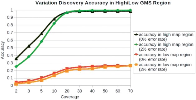
We measured the Variation Discovery Accuracy test on 20 experiments. 0% Error rate is used as a control group so that only the effect of mutation remains. The accuracy of the 0% error rate outperforms that of 2% error rate but by a very small margin at 30-fold coverage. Given sufficient coverage, the accuracy rate is close to 100%, in high GMS region, while it cannot be improved in low GMS region, even though high level of coverages are used. Therefore, 28% detection efficiency is the upper limit in low GMS region using current sequencing technology

That means that unlike typical false negatives, increasing coverage will not help identify mutations in low GMS regions, even with 0% sequencing error. Instead, this is because the SNP-calling algorithms use the mapping quality scores to filter out unreliable mapping assignments, and low GMS regions have low mapping quality score (by definition). Thus, even though many reads may sample these variations, the mapping algorithms cannot ever reliably map to them. Since about 14% of the genome has low GMS value with typical sequencing parameters, it is expected that about 14% of all variations of all resequencing studies will not be detected. To demonstrate this effect, we characterised the SNP variants identified by the 1000 genomes pilot project, and found that 99.99% of the SNPs reported were in high GMS regions of the genome, and in fact 99.95% had GMS over 90.

The results from the 1000 Genomes project and our VAS experiments are alarming for projects using sequencing to identify causal mutations because low GMS regions occur throughout the human genome, throughout the exome, and even include clinically relevant SNPs (Supplementary Table S2). In particular, within the low GMS regions, there are important variations (Supplementary Table S3) such as rs33992775 (GMS:0.00) related to hemoglobin, rs104893928 (GMS:0.00) related to survival of motor neurons, rs116840812 (GMS:0.00) related to ribosomal proteins and so on. The frequency of known SNPs and known clinically relevant SNPs is heavily biased away from the low GMS regions: only 0.03% of all known SNPs and only 0.14% of all known clinically relevant SNPs occur in low GMS regions even though 8.74% of the genome and 0.92% of the transcribed bases have low GMS bases. This is not at all surprising, since existing catalogs of variations have been constructed using methods that face inherent and unavoidable limitations and can only be addressed by using radically different sequencing technology.

4 DISCUSSION

Short read mapping has become one of the most important tools in molecular biology, with many significant applications to understanding human health and disease, plant and animal genomics and basic biological processes. The algorithms for efficiently mapping reads to the genome are now rapidly maturing, but until now it was an open question of how to interpret the reliability of those mappings. Prior working focusing on the mapping quality score or the Uniqueome were narrowly focused on individual reads or individual subsequences and missed the larger genomic context.

Here, we have presented a novel probabilistic metric, the GMS for identifying and quantifying the regions of the genome that can be reliably mapped under various experimental conditions. We have also developed the GMA pipeline for computing the GMS profile of a genome, leveraging Hadoop to accelerate the computation to genomes of any size. Using the GMA pipeline, we have identified that 14% of the human genome and 4% of the known transcribed region has low GMS values in which variations will be difficult or impossible to measure given today's sequencing technology. Furthermore, our analysis of the widely used BWA + SAMtools single nucleotide polymorphism detection algorithm shows that most SNP detection errors are false negatives, and most of the missing variations are in regions with low GMS scores. These types of errors are fundamental to the genome composition, and cannot be overcome by merely increasing coverage. Notably, the vast majority of variations reported by the 1000 Genomes project are within high GMS regions and nearly none is reported in low GMS regions.

These results highlight the importance of measuring the GMS profile when analyzing the results of resequencing studies, especially when interpreting the degree or distribution of variations within the genome. Without considering the GMS, an analysis may falsely conclude that certain regions of the genome do not undergo mutations, while in fact through an unavoidable limitation of the resequencing method, the experiments have no power to measure those variations. These hidden mutations in the genomic dark matter may play a very significant role to disease analysis.

It remains for future work to fully integrate the GMS profile into a full genotyping solution. For example, a major challenge in detecting structural variations is reconciling putative mutations with repeat elements. The GMS profile could be used to identify regions of the genome that can be confidently measured, and poorly mappable regions can be filtered from the analysis.

REFERENCES

- 1000 Genomes Project Consortium A map of human genome variation from population-scale sequencing. Nature. 2010;467:1061–1073. doi: 10.1038/nature09534. [DOI] [PMC free article] [PubMed] [Google Scholar]
- Bentley D.R., et al. Accurate whole human genome sequencing using reversible terminator chemistry. Nature. 2008;456:53–59. doi: 10.1038/nature07517. [DOI] [PMC free article] [PubMed] [Google Scholar]
- Burrows M., Wheeler D.J. A block-sorting lossless data compression algorithm. Technical Report Digitial SRC Research Report 124. 1994 [Google Scholar]
- Carlton J.M., et al. Draft genome sequence of the sexually transmitted pathogen. Trichomonas vaginalis. Science. 2007;315:207–212. doi: 10.1126/science.1132894. [DOI] [PMC free article] [PubMed] [Google Scholar]
- Dean J., Ghemawat S. Symposium on Operating System Design and Implementation (OSDI) 2004. MapReduce: simplified data processing on large clusters; pp. 137–150. [Google Scholar]
- Drmanac R., et al. Human genome sequencing using unchained base reads on self-assembling DNA nanoarrays. Science (New York, N.Y.) 2010;327:78–81. doi: 10.1126/science.1181498. [DOI] [PubMed] [Google Scholar]
- ENCODE Project Consortium The ENCODE (ENCyclopedia Of DNA Elements) project. Science. 2004;306:636–640. doi: 10.1126/science.1105136. [DOI] [PubMed] [Google Scholar]
- Gilles A., et al. Accuracy and quality assessment of 454 GS-FLX Titanium pyrosequencing. BMC Genom. 2011;12:245. doi: 10.1186/1471-2164-12-245. [DOI] [PMC free article] [PubMed] [Google Scholar]
- Grad Y.H., et al. Genomic epidemiology of the Escherichia coli O104:H4 outbreaks in Europe, 2011. Proc. Nat. Acad. Sci. 2012;109:3065–3070. doi: 10.1073/pnas.1121491109. [DOI] [PMC free article] [PubMed] [Google Scholar]
- Holtgrewe M., et al. A novel and well-defined benchmarking method for second generation read mapping. BMC Bioinformatics. 2011;12:210. doi: 10.1186/1471-2105-12-210. [DOI] [PMC free article] [PubMed] [Google Scholar]
- International Cancer Genome Consortium International network of cancer genome projects. Nature. 2010;464:993–998. doi: 10.1038/nature08987. [DOI] [PMC free article] [PubMed] [Google Scholar]
- International Human Genome Sequencing Consortium Initial sequencing and analysis of the human genome. Nature. 2001;409:860–921. doi: 10.1038/35057062. [DOI] [PubMed] [Google Scholar]
- Koehler R., et al. The Uniqueome: a mappability resource for short-tag sequencing. Bioinformatics. 2010;27:272–274. doi: 10.1093/bioinformatics/btq640. [DOI] [PMC free article] [PubMed] [Google Scholar]
- Koren S., et al. Hybrid error correction and de novo assembly of single-molecule sequencing reads. Nat. Biotechnol. 2012 doi: 10.1038/nbt.2280. In Press. [DOI] [PMC free article] [PubMed] [Google Scholar]
- Langmead B., et al. Ultrafast and memory-efficient alignment of short DNA sequences to the human genome. Genome Biol. 2009;10:R25. doi: 10.1186/gb-2009-10-3-r25. [DOI] [PMC free article] [PubMed] [Google Scholar]
- Li H., Durbin R. Fast and accurate short read alignment with BurrowsWheeler transform. Bioinformatics. 2009;25:1754–1760. doi: 10.1093/bioinformatics/btp324. [DOI] [PMC free article] [PubMed] [Google Scholar]
- Li H., et al. The sequence alignment/map format and SAMtools. Bioinformatics. 2009a;25:2078–2079. doi: 10.1093/bioinformatics/btp352. [DOI] [PMC free article] [PubMed] [Google Scholar]
- Li H., et al. Mapping short DNA sequencing reads and calling variants using mapping quality scores. Genome Res. 2008;18:1851–1858. doi: 10.1101/gr.078212.108. [DOI] [PMC free article] [PubMed] [Google Scholar]
- Li R., et al. SOAP2: an improved ultrafast tool for short read alignment. Bioinformatics (Oxford, England) 2009b;25:1966–1967. doi: 10.1093/bioinformatics/btp336. [DOI] [PubMed] [Google Scholar]
- modENCODE Consortium Identification of functional elements and regulatory circuits by Drosophila modENCODE. Science (New York, N.Y.) 2010;330:1787–1797. doi: 10.1126/science.1198374. [DOI] [PMC free article] [PubMed] [Google Scholar]
- Rothberg J.M., et al. An integrated semiconductor device enabling non-optical genome sequencing. Nature. 2011;475:348–352. doi: 10.1038/nature10242. [DOI] [PubMed] [Google Scholar]
- Schatz M.C., et al. Cloud computing and the DNA data race. Nat. Biotechnol. 2010;28:691–693. doi: 10.1038/nbt0710-691. [DOI] [PMC free article] [PubMed] [Google Scholar]
- Shvachko K., et al. 2010 IEEE 26th Symposium on Mass Storage Systems and Technologies (MSST) 2010. The hadoop distributed file system; pp. 1–10. [Google Scholar]
- Stein L.D. The case for cloud computing in genome informatics. Genome Biol. 2010;11:207. doi: 10.1186/gb-2010-11-5-207. [DOI] [PMC free article] [PubMed] [Google Scholar]
Associated Data
This section collects any data citations, data availability statements, or supplementary materials included in this article.