A varying-coefficient method for analyzing longitudinal clinical trials data with nonignorable dropout

Abstract

Dropout is common in longitudinal clinical trials and when the probability of dropout depends on unobserved outcomes even after conditioning on available data, it is considered missing not at random and therefore nonignorable. To address this problem, mixture models can be used to account for the relationship between a longitudinal outcome and dropout. We propose a Natural Spline Varying-coefficient mixture model (NSV), which is a straightforward extension of the parametric Conditional Linear Model (CLM). We assume that the outcome follows a varying-coefficient model conditional on a continuous dropout distribution. Natural cubic B-splines are used to allow the regression coefficients to semiparametrically depend on dropout and inference is therefore more robust. Additionally, this method is computationally stable and relatively simple to implement. We conduct simulation studies to evaluate performance and compare methodologies in settings where the longitudinal trajectories are linear and dropout time is observed for all individuals. Performance is assessed under conditions where model assumptions are both met and violated. In addition, we compare the NSV to the CLM and a standard random-effects model using an HIV/AIDS clinical trial with probable nonignorable dropout. The simulation studies suggest that the NSV is an improvement over the CLM when dropout has a nonlinear dependence on the outcome.

1. Introduction

Dropout in longitudinal clinical trials occurs for reasons that may be related to the outcome of interest. For example, in HIV/AIDS studies patients may experience drug-related toxicities or develop viral resistance to therapy. These reasons can be related to an outcome, such as CD4⁺ T cell count, a measure of immunologic health. When the reason for dropout is associated with the unmeasured values of the outcome of interest, missing data are said to be missing not at random (MNAR) and are therefore nonignorable [1,2]. Traditional methods, such as mixed- or random-effects models (REM) [3], ignore the dropout mechanism. The analysis method must account for the outcome-dropout relationship as ignoring MNAR data can lead to biased results [1,2]. A thorough review is provided by Hogan, Roy and Korkontzelou, 2004 [4].

Mixture models assume that the trajectory of the outcome is a function of dropout time. For example, individuals who drop out earlier may have steeper declines over time. We consider mixture models in applicable settings where the longitudinal trajectories are roughly linear over time, the time of dropout is observed for all individuals and observations are mistimed such that dropout can be considered continuous. These approaches further assume that intermittent missing data are missing at random, there is variability in the slope among subjects and subjects who complete the study behave as if they dropped out immediately after that point in time. Wu and Bailey’s conditional linear model (CLM) is an established mixture model method that assumes the regression coefficients are polynomial (parametric) functions of dropout time [5]. These parametric models often result in a poor fit of the relationship between dropout time and the individual trajectories. Hogan, Lin and Herman (2004) [6] propose a semi-parametric varying-coefficient mixture model with a roughness penalty that estimates the smoothing parameter as an extra variance component [7,8]. While flexible, this method is not trivial to implement, can suffer from convergence problems and requires multiple groups be fit separately for numerical stability. We propose a numerically stable Natural Spline Varying-coefficient (NSV) mixture model approach which uses natural cubic B-spline basis functions in the fixed effects. The NSV was developed to provide a flexible method for modeling the outcome-dropout relationship and to avoid potential bias resulting from an incorrectly specified parametric dropout mechanism. This method is a straightforward extension of the CLM and uses standard statistical software.

The details of the CLM and NSV methods are presented in Sections 2.3 and 2.4, respectively. A simulation study which assesses model performance when assumptions are met and violated is detailed in Section 3 and a clinical trial application using an HIV/AIDS dataset is described in Section 4. Conclusions follow in Section 5.

2. Methods

2.1. Conditional model

Mixture models account for the dropout mechanism by factoring the joint outcome-dropout distribution into the dropout-time distribution, f(u), and the distribution of the outcome given dropout, f(y|u). The resulting complete data distribution, f(y), is ∫f(y|u)dF(u). We assume m subjects with n_i observations measured over time, $\text{t}={({\text{t}}_1^T,\dots ,{\text{t}}_{\text{m}}^T)}^T$ and assuming the curves vary with dropout time, we anticipate significant individual variation (intercepts and slopes). The conditional model of the N × 1 outcome vector, Y, given dropout times u can be written as the mixed-effects dropout-varying coefficient model:

$$(\text{Y}\mid U)={\beta }_0(\text{u})+{\beta }_1(\text{u})\ast \text{t}+\text{Zb}+\epsilon ,$$ (1)

where * represents an elementwise product of the vectors. The dropout-varying intercept (k = 0) and slope (k = 1) are ${\beta }_k(\text{u})={({\beta }_{1k}^T,\dots ,{\beta }_{mk}^T)}^T$, where β_ik = I_iβ_k(u_i) and I_i is an n_i × 1 vector of 1’s. Z is the design matrix associated with the random effects b ~ N(0, D) and is independent from the residual error, ε ~ N(0, R).

2.2. Marginal estimates

For each group, h = {1, …, s}, we estimate the marginal coefficients (intercept and slope). We define ${\text{u}}_h^0=(u_{1_h}^0,\dots ,u_{r_h}^0)$ as the r_h unique ordered dropout times for the hth group and Ĩ_hi to be an r_h × 1 dropout time indicator vector for u_hi, the ith patient’s dropout time in the hth group. The hth group’s marginal coefficients are

$${\widehat{\beta }}_{hk}^{\ast }=\int {\widehat{\beta }}_{hk}(u_h)d\widehat{F}(u)={\widehat{\pi }}_h^T\widehat{\beta }\left({\text{u}}_h^0\right).$$ (2)

Here, F̂(u) is the empirical cdf of u and ${\widehat{\beta }}_{hk}({\text{u}}_h^0)$ is the r_h × 1 vector of smooth function values. Additionally, ${\widehat{\pi }}_h={\displaystyle \sum _{i=1}^{m_h}}\frac{{\stackrel{\sim }{\text{I}}}_{hi}}{m_h}$, where m_h is the number of subjects in the hth group.

2.3. Conditional linear model

The CLM [5] was developed to compare slopes across treatment groups.

For the hth group and the ith subject, with Z_i = [1, t_i],

$$({\text{Y}}_i\mid U=u_i)=\sum _{j=0}^{J_{h0}}{\theta }_{hj0}{u}_{hi}^j\ast {\text{I}}_i+\sum _{j=0}^{J_{h1}}{\theta }_{hj1}{u}_{hi}^j\ast {\text{t}}_i+{\text{Z}}_i{\text{b}}_i+{\epsilon }_i.$$ (3)

Wu and Bailey [5] constrained J_h0 = 0, resulting in a constant (not dropout-varying) intercept, such that β_h0(u-_hi) = θ_h00 for all subjects. The ith subject’s dropout-varying slope is ${\beta }_{h1}(u_{hi})={\sum }_{j=0}^{J_{h1}}{\theta }_{hj1}{u}_{hi}^j$. This model can easily be written in the form of Eq. (1). Although relatively simple to implement, simple polynomial functions may lack the flexibility necessary to adequately fit the dropout mechanism. Additionally, if the parametric specification for the dropout mechanism is incorrect, the results will be biased [6,9].

2.4. Natural spline varying-coefficient model

Ideally, a mixture model method would be data driven and not require a parametric specification. Therefore, we propose a semiparametric Natural Spline Varying-coefficient (NSV) approach. This method relies on natural cubic B-spline basis functions to model the dropout mechanism. Standard B-spline basis functions are flexible, nearly orthogonal, numerically stable, easy to compute and possess local support [10–12]. The linear constraint beyond the boundary knots provided by natural cubic B-splines (as opposed to standard B-splines) improve model behavior if data are sparse near the boundaries. The conditional NSV model is

$$({\text{Y}}_i\mid U=u_i)=\sum _{j=0}^{J_{h0}}{\theta }_{hj0}{\stackrel{\sim }{u}}_{\mathit{hij}0}\ast {\text{I}}_i+\sum _{j=0}^{J_{h1}}{\theta }_{hj1}{\stackrel{\sim }{u}}_{\mathit{hij}1}\ast {\text{t}}_i+{\text{Z}}_i{\text{b}}_i+{\epsilon }_i,$$ (4)

where ũ_hijk = B̃(u_h, J_hk)_{[i, j+1]} for k = 0,1. For j > 0, B̃(u_h, J_hk) is the matrix of basis functions with J_hk degrees of freedom (df) and B̃(u_h, J_hk)_[,1] is 1. Respectively, the ith subject’s dropout-varying intercept and slope are

$${\beta }_{hi0}=\sum _{j=0}^{J_{h0}}{\theta }_{hj0}{\stackrel{\sim }{u}}_{\mathit{hij}0}=\sum _{j=0}^{J_{h0}}{\theta }_{hj0}\stackrel{\sim }{B}{({\text{u}}_h,J_{h0})}_{[i,j+1]},$$ (5)

$${\beta }_{hi1}=\sum _{j=0}^{J_{h1}}{\theta }_{hj1}{\stackrel{\sim }{u}}_{\mathit{hij}1}=\sum _{j=0}^{J_{h1}}{\theta }_{hj1}\stackrel{\sim }{B}{({\text{u}}_h,J_{h1})}_{[i,j+1]}.$$ (6)

We define β_hk(u_hi) = I_iβ_hik. We can then re-write the subject-specific model as

$$({\text{Y}}_i\mid U=u_i)={\beta }_{h0}(u_{hi})+{\beta }_{h1}(u_{hi})\ast {\text{t}}_i+{\text{Z}}_i{\text{b}}_i+{\epsilon }_i.$$ (7)

Stacking these models results in a mixed-model for the full data (Eq. (1)). The B-spline knots (df − 1) are based on the hth set of dropout times and the df determine model flexibility and the number of parameters. This semiparametric method differs from the CLM by using natural cubic B-spline transformations of dropout time rather than polynomial transformations and additionally allows for a dropout-varying intercept.

Subjects with early dropout times contribute fewer observations and estimates of their trajectories are less stable. To increase stability, we take advantage of the linearity of the natural cubic B-splines below the lower boundary, which we now denote as d_Lh. Above, d_Lh was assumed to be the first drop-out time (u_1h⁰). An offset can be incorporated, shifting the lower boundary (d_Lh > u_1h⁰) such that the coefficients in this region, u ∈ [u_1h⁰, d_Lh], will change linearly as a function of drop-out time and provide stability. Eq. (5) now utilizes the following basis functions: for l = {0,1} and j > 0, B̃(u_h, J_hl, d_Lh), is the matrix of basis functions with lower boundary d_Lh.

3. Simulation study

We assess model performance using simulation studies similar to those described in Hogan, Lin and Herman (2004) [6]. The NSV and CLM rely on the assumption that the β_k(u) are continuous and smooth as a function of dropout time. The simulation studies included three functional forms for the dropout mechanism. Form (i) is continuous and smooth, meeting the NSV assumptions. Form (ii) is continuous but not smooth, initially increasing then forming a plateau. Lastly, form (iii) violates both smoothness and continuity and is generated from a step function, which may be difficult for the models to capture. We also considered how within-subject variability impacts model performance by simulating two variance settings.

We assume the following form for the data:

$$y_{ij}={\beta }_0(u_i)+{\beta }_1(u_i)t_{ij}+a_{0i}+a_{1i}{t}_{ij}+{\epsilon }_{ij},i=1,\dots ,m;j=1,\dots ,n_i,$$

for m subjects with n_i observations for the ith subject, where (a_0i, a_1i)^T ~ N (0, D), ε_ij ~ N(0, σ²) and β₀(u) = 0. Dropout is created from a beta-binomial where p~Beta(1.5,1.5) and U~Bin(15, p). Dropout times are u = U/15 ∈ [0,1], resulting in 16 timepoints spaced equally from 0 to 1.

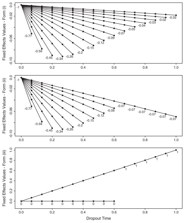
The forms of the dropout mechanism, β₁(u), are: (i) −exp(αu), (ii) −exp(αu)I_{(u < t^*)} −exp(αt^*)I_{(u ≥ t^*)} and (iii) α₁I_{(u < t^*)} + α₂I_{(u ≥ t^*)}. We set α = −4 for forms (i) and (ii), define t^* = 2/3 and for form (iii), α₁ = 0 and α₂ = 1. Fig. 1 displays the dropout-specific slopes for each model. The within-subject variance, σ², is 0.067 and 0.2 for the small and large settings, respectively.

Fig. 1.

Simulation study: dropout-specific slopes. For simulation forms (i), (ii) and (iii), the dropout-specific slopes are plotted and the value of the slope indicated.

For each form/variance combination, 1000 datasets with 400 subjects each were created and the elements of D are as follows: d₁₁ = 0.4, d₂₂ = 0.01 and d₁₂ = −0.01.

We fit an NSV, CLM and REM to each dropout-form/variance combination. For each simulated dataset, AIC was used to determine the number of B-spline knots. We considered a maximum of 6 df for each dropout-varying effect and set the left boundary offset, d_L, to 0.20 (corresponding to 4 observations). Likelihood ratio tests were used to select the best CLM, with a cubic polynomial in the full model (J₁ = 3).

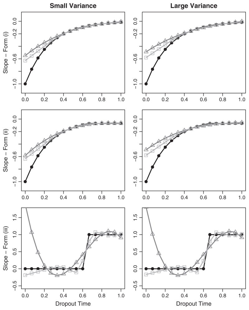
We graphically assess performance by plotting the means of the β̂₁(u_i) for the NSV and CLM models against the true slope, β₁(u_i), at each dropout time (Fig. 2). These graphs demonstrate that the NSV fits the β₁(u_i) for forms which meet and violate model assumptions. In form (iii), the step function, the NSV demonstrates surprising performance given the assumption violations. A cubic polynomial predominates in the CLM for form (iii), resulting in a poor fit in the region of the early dropout times. For all forms and dropout times, the NSV performs better or comparable to the CLM.

Fig. 2.

Simulation study: performance of the dropout models. For simulation forms (i), (ii) and (iii), the mean of the dropout-varying slopes for the NSV (□– □), and CLM (△– △) are plotted against the true slopes (● – ●). The x-axis is dropout time and the y-axis is the slope value.

We next quantify performance of the marginal model for the slopes by calculating the mean squared error (MSE) of the marginal slope, ${\widehat{\beta }}_1^{\ast }$. For the jth dataset, MSE is ${\left({\beta }_1^{\ast }-{\widehat{\beta }}_{1j}^{\ast }\right)}^2$, where ${\beta }_1^{\ast }$ is the true marginal slope. The MSE geometric means and 95% confidence intervals are displayed in Table 1. For all form/variance combinations, the NSV MSE is the smallest, supporting the results shown in Fig. 2. Table 2 displays the mean estimated marginal slope for each method. Again, the NSV demonstrates superior performance as compared to the CLM. As anticipated, the REM is outperformed by both mixture models. In summary, the NSV method is computationally tractable, numerically stable and provides reliable estimates under a variety of dropout mechanisms.

Table 1.

Simulation study: MSE geometric means. Estimates are based on n = 1000 simulations.

Form — variance	NSV	CLM	REM
i-Small	0.0025 (0.0022, 0.0028)	0.0034 (0.0030, 0.0038)	0.029 (0.028, 0.029)
i-Large	0.0047 (0.0041, 0.0054)	0.0051 (0.0044, 0.0058)	0.029 (0.028, 0.030)
ii-Small	0.0023 (0.0020, 0.0026)	0.0031 (0.0027, 0.0035)	0.024 (0.023, 0.024)
ii-Large	0.0054 (0.0047, 0.0061)	0.0061 (0.0054, 0.0069)	0.023 (0.023, 0.024)
iii-Small	0.0023 (0.0020, 0.0026)	0.0096 (0.0086, 0.011)	0.068 (0.067, 0.070)
iii-Large	0.0060 (0.0053, 0.0069)	0.0096 (0.0083, 0.011)	0.0137 (0.135, 0.14)

Table 2.

Simulation study: mean marginal slopes. Estimates are based on n = 1000 simulations.

Form - Variance	True Slope ${\beta }_1^{\ast }$	NSV	CLM	REM
i-Small	−0.234	−0.201	−0.184	−0.064
i-Large	−0.234	−0.192	−0.174	−0.061
ii-Small	−0.243	−0.211	−0.196	−0.088
ii-Large	−0.243	−0.200	−0.180	−0.086
iii-Small	0.347	0.331	0.472	0.612
iii-Large	0.347	0.333	0.466	0.721

4. Application

4.1. HIV clinical trial

We analyzed data from a double-blind, randomized HIV/AIDS clinical trial that evaluated treatment with mono-therapy lamivudine (3TC) or zidovudine (AZT); or dual-therapy including either a low or high dose of 3TC (AZT+3TC low and AZT+3TC high) [13]. Three hundred sixty-six subjects, with CD4⁺ T cell count between 200 and 500 cells per cubic millimeter, were randomized to the four treatment groups and followed for up to 100 weeks. Eron et al. (1995) described the data through week 52, and based on HIV-1 RNA (viral load), demonstrate that dual-therapy was superior. Our outcome of interest, CD4⁺ T cell count, was measured every 4 weeks through week 52 and every 8 weeks thereafter. We defined our two treatment groups as mono-therapy (AZT and 3TC arms; n = 180) and dual-therapy (AZT+3TC low and AZT+3TC high arms; n = 186). The mono-therapy and dual-therapy groups had a median (range) of 14 (1, 20) and 13 (1, 20) observations per subject, respectively, with corresponding median last visits of 53 (0, 100) and 52 (0, 100) weeks. For each subject, dropout time was defined as the last visit plus one day. Thus, all subjects had an observed dropout time.

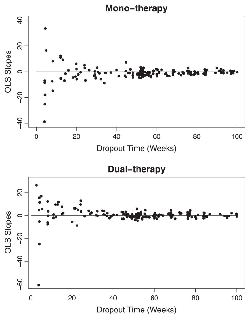
We began the investigation of the dependence of individual rates of change on time of dropout by plotting the ordinary least squares (OLS) slopes by dropout time for the two groups (Fig. 3). While the dropout mechanism was unclear for the mono-therapy group, subjects with a positive slope (increasing CD4⁺ T cell counts) tended to drop out early in the dual-therapy group as indicated by the greater number of points above 0 over the first 30 to 40 weeks. Adherence to drug can result in both treatment-related toxicities and better outcomes (positive CD4⁺ T cell slope). Therefore it is biologically plausible that subjects who are adhering to treatment in the dual-therapy arm have positive slopes and are also likely to drop out early due to toxicities.

Fig. 3.

HIV clinical trial: OLS slopes. For each treatment group, the OLS slopes are plotted by dropout time, as obtained from individual-specific models of CD4⁺ T cell count as a linear function of time.

4.2. Dropout models

4.2.1. NSV

CD4⁺ T cell count was modeled as a function of treatment group and time with group-specific dropout-varying B-spline bases for the intercepts and slopes in the fixed effects and a random subject-specific intercept and slope. Considering the full model with maximum df, likelihood ratio tests justified including a parameter for the covariance of the subject-specific random effects and confirmed the presence of significant individual slope variation. We allowed each group’s dropout-varying intercept, β_h0(u_h), and slope, β_h1(u_h), to have its own flexibility (J_hk). Based on the median number of observations per subject (13–14) and to limit the potential for over fitting, we considered a range of 0–6 and 1–6 df for each intercept and slope, respectively. For stable slope estimation, we set a lower boundary offset for each group’s dropout-varying intercept and slope to week 12 plus one day (corresponding to 4 observations). We located the B-spline knots at the quantiles of u_h > d_Lh, the hth group’s set of unique dropout times greater than the lower boundary [7,10]. As we are interested in estimation, Akaike’s Information Criterion (AIC) determined the final model [12,14]. The natural cubic B-spline basis functions were produced using the ns() function in R and the models were fit using the lmer() function [15]. The best AIC model included 3 (1) df for the dropout-varying mono-therapy intercept (slope) and 1 (3) df for the dropout-varying dual-therapy intercept (slope).

4.2.2. CLM

CD4⁺ T cell count was modeled as a function of treatment group and time, with group-specific dropout-varying slopes and a random subject-specific intercept and slope. As previously described, the CLM assumes a dropout-varying slope with a constant intercept (with respect to dropout). Thus, we began with a cubic polynomial to model the dropout-varying slope where J_h0 = 0 and J_h1 = 3. Likelihood ratio tests confirmed significant individual slope variation and justified including a parameter for the covariance of the subject-specific random effects. The final model included a linear dropout-varying slope for both treatment groups (CLM1). We fit a second CLM (CLM2), allowing for a dropout-varying intercept for each group and we began with J_h0 = 3 and J_h1 = 3. The final model included a linear dropout-varying mono-therapy intercept and a constant dual-therapy intercept. The dropout-varying slope for both groups was linear, as with CLM1. The models were fit using both SAS Proc Mixed [16] and the R lmer() function [15].

4.3. Dropout-varying estimates

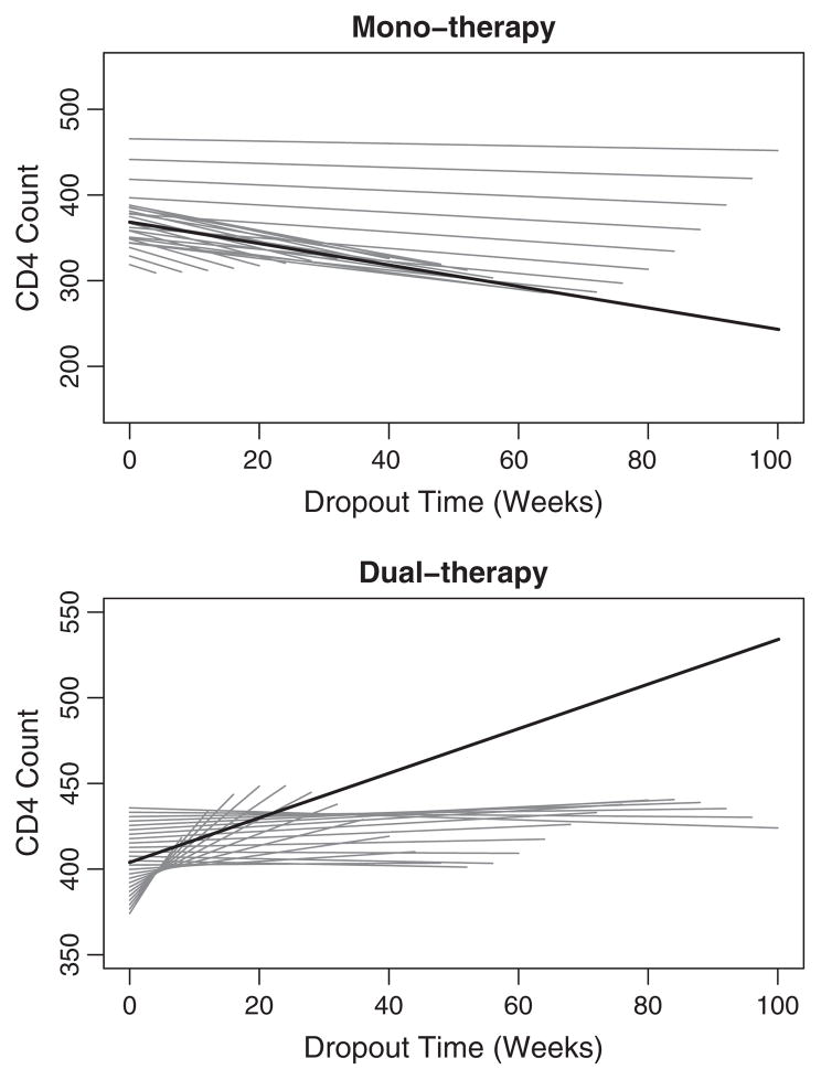
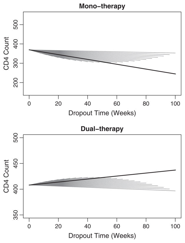
The dropout-varying slopes for 12-week increments are displayed in Table 3. Figs. 4 and 5 display the dropout-specific curves for the NSV and CLM1 respectively. The dropout-specific curves for the CLM2 are similar to those of the CLM1 and are therefore not shown. The NSV mono-therapy intercept was lowest for early dropout times and increased markedly after week 72, indicating that subjects who began the study with higher CD4⁺ T cell count (less immunocompromised) stayed on study longer. The same effect, but diminished, was present in a gradual linear (1df) increase of the NSV dual-therapy dropout-varying intercept. The NSV mono-therapy dropout-varying slope was similar for the NSV and CLMs, both were negative for all dropout times and approach zero with increasing follow-up. For the NSV dual-therapy group, the rate of change in CD4⁺ T cell count was positive through dropout week 48, though the slope flattened substantially over this time. This suggests that subjects who initially dropped out were in the effective treatment period and over time viral resistance may be occurring. A plausible explanation is that compliance is associated with both improved response (positive slope) and treatment-related toxicities, the latter resulting in dropout. The CLM1 and CLM2 dual-therapy dropout-varying slope estimates are also positive, though substantially flatter through week 40 than the NSV.

Table 3.

HIV clinical trial: estimated dropout-varying slopes.

Dropout week	Mono			Dual
	NSV	CLM1	CLM2	NSV	CLM1	CLM2
12	−2.22	−2.19	−2.12	4.53	0.604	0.603
24	−1.94	−1.92	−1.86	2.57	0.506	0.505
36	−1.66	−1.64	−1.59	0.949	0.408	0.408
48	−1.37	−1.37	−1.33	0.024	0.311	0.310
60	−1.09	−1.09	−1.06	−0.014	0.213	0.213
72	−0.801	−0.813	−0.799	0.211	0.115	0.115
84	−0.571	−0.537	−0.535	0.180	0.018	0.017
96	−0.232	−0.261	−0.271	−0.031	−0.080	−0.080

Fig. 4.

HIV clinical trial: NSV dropout-varying and marginal curves. Mono-therapy and dual-therapy dropout-varying curves are plotted by dropout time with line length indicating duration of follow-up. The marginal curve is denoted by the solid blackline.

Fig. 5.

HIV clinical trial: CLM dropout-varying and marginal curves. Mono-therapy and dual-therapy dropout-varying curves are plotted by dropout time with line length indicating duration of follow-up. The marginal curve is denoted by the solid blackline.

4.3.1. Marginal estimates

For the NSV and CLM1, the estimated marginal curves are displayed in Figs. 4 and 5; and for all methods, the estimated marginal slopes and group differences are displayed in Table 4, with bootstrap 95% confidence intervals where appropriate [17]. Estimates from a random effects model (REM) are included for comparison. For the estimate of interest, the slope difference, all methods suggest that the dual therapy arm is superior. CD4⁺ T Cell count consistently declined in the mono-therapy group and increased in the dual-therapy group regardless of the method of estimation. For the dual-therapy group, the NSV final model included a nonlinear dropout-varying slope. The resulting marginal slope was the most positive among the model estimates, reflecting the slopes of the dropouts prior to week 40. In contrast, the CLM1 and CLM2 final models were linear, diminishing the impact of these earlier dropouts on the marginal slope. Finally, the REM marginal estimate was closest to zero due to the increased data contribution of subjects with the longest follow-up. For mono-therapy, both the NSV and CLMs were linear in the dropout-varying slopes. The impact of the linear dropout-varying intercept on the marginal estimate in the CLM2 is negligible. Again, the REM estimate was most similar to the slopes of the subjects with the most data.

Table 4.

HIV Clinical Trial: Estimated Marginal Slopes.

Model	Bootstraps	Mono (95% CI)	Dual (95% CI)	Difference (95% CI)
NSV	1000	−1.25 (−1.69, −0.88)	1.30 (0.43, 2.27)	−2.55 (−3.67, −1.64)
CLM1	1000	−1.25 (−1.62, −0.87)	0.29 (−0.14, 0.70)	−1.54 (−2.08, −0.95)
CLM2	1000	−1.22 (−1.30, −1.13)	0.29 (0.26, 0.32)	−1.51 (−1.60, −1.41)
REM	NA	−0.89 (−1.17, −0.60)	0.14 (−0.15, 0.43)	−1.03 (−1.44, −0.60)

4.4. Sensitivity analyses

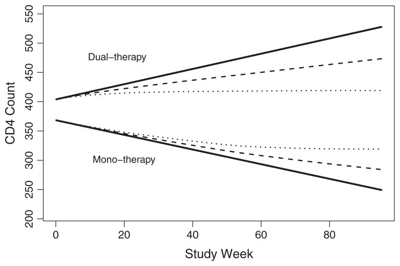
Both the NSV and CLM assume that changes in CD4⁺ T cell count after treatment initiation is linear, which is consistent with knowledge of treatment effects at the time of this study. Since this study, it has been established that changes in CD4⁺ T cell count may be nonlinear after treatment initiation. Sensitivity analyses were conducted. Given data through time u, we estimate the dropout specific slope for time u and assume the same slope for times t > u. Although the change in the slope is nonidentifiable, we evaluate the impact of a specific change in the slope, δ(u), for times t > u. Ideally, analyses will be robust to reasonable changes in δ(u). We conservatively chose changes in the slope to be more consistent with the null hypothesis. We set δ(u) = 0.5 for the first analysis and for the second, we assume all subjects’ slopes flatten to zero for times t > u. The average estimate across all subjects was then calculated for each week (Fig. 6). This allows evaluation of the impact on between group differences in the outcome at specified times. Fig. 6 suggests that for both assumptions, the dual-therapy arm is superior at one year and at study completion.

Fig. 6.

HIV clinical trial: NSV sensitivity analysis. Marginal estimates are plotted for dual-therapy (top curves) and mono-therapy (bottom curves) with three different assumptions after subjects drop out. The solid black lines indicate the final model, which assumes subjects continue with the same trajectory after dropping out. The dashed lines assume subjects’ slopes flatten by 1/2 and the dotted line assumes subjects’ slopes flatten to zero.

5. Conclusions

We propose a straightforward varying-coefficient model using natural cubic B-spline basis functions (NSV) to semipara-metrically model the outcome-dropout relationship in longitudinal clinical trials where nonignorable dropout is probable. We compare this method as an alternative to an existing mixture model, the parametric CLM [5]. Simulation studies suggest the NSV is an improvement over the CLM when the dropout mechanism is nonlinear.

The NSV brings a variety of strengths including computationally stability and simultaneous modeling of multiple groups. It is highly flexible, provides control over the degree of smoothness for each effect and is relatively simple to implement using standard software. Use of natural cubic B-splines increases stability beyond the boundaries and allows incorporation of a lower boundary offset, extending stability to slope estimation for the early dropouts. Additionally, as the NSV is data driven, it is not necessary to pre-specify the parametric model for the dropout mechanism. This is particularly useful in trials where the analytic plan must be established prior to examining the data. The conditional model can also be evaluated for clinical relevance by plotting the dropout-varying curves, which can lend credibility to the model and provide the opportunity for critical evaluation of the dropout mechanism. Plots similar to Fig. 4 can be examined to assess the clinical feasibility of the dropout model. Lastly, as with all with a mixture model approaches, the missing data extrapolations are transparent and can be graphically presented (for a review, see Hogan, Roy and Korkontzelou, 2004) [4].

There are limitations to the NSV, as with all methods for nonignorable dropout. The mixture models considered in this paper assume that trajectories are linear over time and extrapolate based on this assumption beyond the dropout time. This is a strong, untestable assumption. One must rely on clinical justification and judgment as to whether the assumption is reasonable [9] and sensitivity analyses should be performed. Future research will include simulation studies to allow for non-linear trajectories over time, refine the B-spline knot placement strategy and determine whether a standard NSV model (fixed df) is generally useful.

Abbreviations

3TC

lamivudine

AIC

Akaike’s Information Criterion

AZT

zidovudine

CLM

conditional linear model

HIV-1 RNA

HIV viral load

OLS

ordinary least squares

MNAR

missing not at random

MSE

mean-squared error

NSV

natural spline varying-coefficient model

REM

random-effects model

References

- 1.Little R, Rubin D. Statistical analysis with missing data. New York: John Wiley & Sons; 1987. [Google Scholar]
- 2.Verbeke G, Molenberghs G. Linear mixed models for longitudinal data. New York: Springer-Verlag; 2000. [Google Scholar]
- 3.Laird N, Ware J. Random-effects models for longitudinal data. Biometrics. 1982;38:963–74. [PubMed] [Google Scholar]
- 4.Hogan J, Roy J, Korkontzelou C. Handling drop-out in longitudinal studies. Stat Med. 2004;23:1455–97. doi: 10.1002/sim.1728. [DOI] [PubMed] [Google Scholar]
- 5.Wu M, Bailey K. Estimation and comparison of changes in the presence of informative right censoring; conditional linear model. Biometrics. 1989;45:939–55. [PubMed] [Google Scholar]
- 6.Hogan J, Lin X, Herman B. Mixtures of varying-coefficient models for longitudinal data with discrete or continuous nonignorable dropout. Biometrics. 2004;60:854–64. doi: 10.1111/j.0006-341X.2004.00240.x. [DOI] [PMC free article] [PubMed] [Google Scholar]
- 7.Green P, Silverman B. Nonparametric regression and generalized linear models: a roughness penalty approach. London: Chapman and Hall; 1994. [Google Scholar]
- 8.Zhang D, Lin X, Raz J, Sowers M. Semiparametric stochastic mixed models for longitudinal data. J Am Stat Assoc. 1998;93:710–9. [Google Scholar]
- 9.Fairclough D. Design and analysis of quality of life studies in clinical trials. Boca Raton: Chapman and Hall/CRC; 2002. [Google Scholar]
- 10.Eubank R. Nonparametric regression and spline smoothing. New York: Dekker; 1999. [Google Scholar]
- 11.MacKenzie T, Abrahamowicz M. B-splines without divided differences. Student. 1996;1:223–30. [Google Scholar]
- 12.Hastie T, Tibshirani R. Generalized additive models. Boca Raton: Chapman and Hall/CRC; 1990. [Google Scholar]
- 13.Eron J, Benoit S, Jemsek J, MacArthur R, Santana J, Quinn J, et al. Treatment with lamivudine, zidovudine, or both in HIV positive patients with 200 to 500 CD4+ cells per cubic millimeter. N Engl J Med. 1995;333:1662–9. doi: 10.1056/NEJM199512213332502. [DOI] [PubMed] [Google Scholar]
- 14.Littell R, Milliken G, Stroup W, Wolfinger R. SAS for mixed models. 2. Cary NC: SAS Institute Inc; 2006. [Google Scholar]
- 15.R Development Core Team. Vienna, Austria: R Foundation for Statistical Computing. 2006. A Language and Environment for Statistical Computing. 3-900051-07-0. [Google Scholar]
- 16.SAS Institute, Inc. SAS 9.1.3 help and documentation. Cary, NC: SAS Institute Inc; 2000–2004. [Google Scholar]
- 17.Efron B, Tibshirani R. An introduction to the bootstrap. In: Cox D, et al., editors. Monographs on statistics and applied probability. Vol. 57. New York: Chapman and Hall/CRC; 1998. [Google Scholar]