Application of an Autoregressive Integrated Moving Average Model for Predicting the Incidence of Hemorrhagic Fever with Renal Syndrome

Abstract

The Box-Jenkins approach was used to fit an autoregressive integrated moving average (ARIMA) model to the incidence of hemorrhagic fever with renal Syndrome (HFRS) in China during 1986–2009. The ARIMA (0, 1, 1) × (2, 1, 0)₁₂ models fitted exactly with the number of cases during January 1986–December 2009. The fitted model was then used to predict HFRS incidence during 2010, and the number of cases during January–December 2010 fell within the model's confidence interval for the predicted number of cases in 2010. This finding suggests that the ARIMA model fits the fluctuations in HFRS frequency and it can be used for future forecasting when applied to HFRS prevention and control.

Introduction

Hemorrhagic fever with renal syndrome (HFRS) is a zoonotic disease caused by different species of hantavirus, which is carried and spread by certain rodents. This disease is highly epidemic in China. Over the past 10 years, 25,000–60,000 HFRS cases were reported annually in China.¹ Because this disease has severe clinical symptoms and high mortality rates, prevention and control are important tasks at all levels at the Center for Disease Control and Prevention in China. However, there is little effect without an integrated rodent control program.

On the basis of a health economics perspective, vaccination is only provided to young adults in areas where the incidence rate is higher than 50 cases/100,000 population (Zhejiang) or 60 cases/100,000 population (Shandong).² Surveillance and early warning are essential for controlling or reducing the risk of outbreaks.³ Early warnings of infectious diseases should be provided on the basis of analysis of surveillance information. These early warnings can provide a scientific basis for better decision making. Thus, it is important to conduct prevention and control programs based on epidemic forecasting.

The autoregressive integrated moving average (ARIMA) model uses the lag and shift of historical information to predict future patterns. The ARIMA model is governed by two factors. The first factor is the length of the historical period that is considered (length of the weight), and the second factor is the specification of the weight value. The ARIMA model is represented as a regression model with a moving average to provide great detail and precision. The ARIMA model was first proposed in 1976 and ARIMA time series intervention analysis is widely used for prediction and early warning analysis of infectious diseases.^4–6

This purpose of this study was to fit ARIMA models and predict the HFRS epidemic trend by using Statistical Package for the Social Sciences (SPSS) version 13.0 (International Business Machines Corporation, Armonk, NY) correlation modules. Our study was based on HFRS epidemic data from the Hebei Province, China, where it could provide a basis for HFRS prevention and control.

Materials And Methods

Materials.

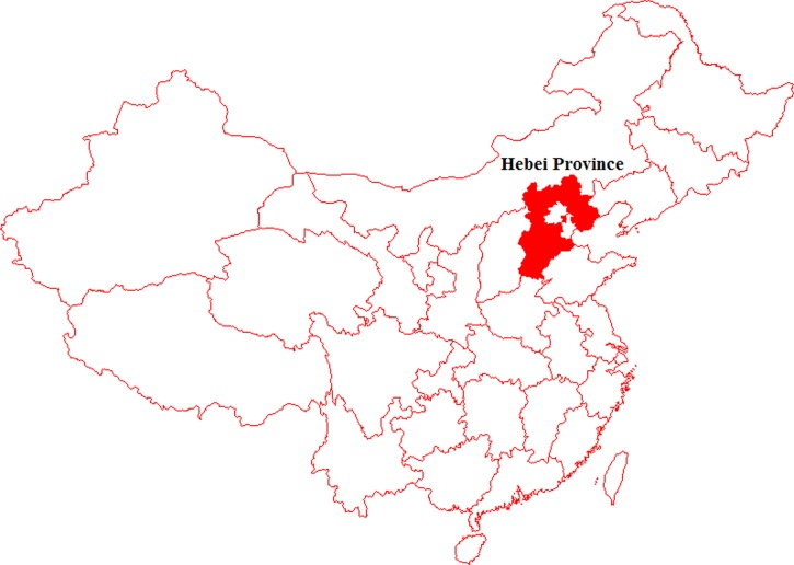
In Hebei Province, the first HFRS case was identified in 1981, and the case record is incomplete until 1986 when systematic data collection commenced. Monthly HFRS cases reported during 1986–2009 in Hebei Province, China (Figure 1), were provided by the Hebei Province Center for Disease Control and Prevention. The data was analyzed by using the appropriate module in SPSS version 13.0.

Figure 1.

Location of Hebei Province, China.

All HFRS cases were initially diagnosed on the basis of clinical symptoms. The typical clinical symptoms include fever, hemorrhage, headache, back pain, abdominal pain, acute renal dysfunction, and hypotension. Patient blood samples were also collected and sent to local Centers for Disease Control and Prevention laboratories for serologic confirmation (detection of IgM). Data were collected by case number according to sampling results. In China, HFRS is a nationally notifiable disease and hospital physicians must report every case of HFRS to the local health authority within 12 hours. Local health authorities send monthly HFRS case reports to the higher national level Center for Disease Control and Prevention for surveillance purposes. Because of mandatory reporting, it is believed that the degree of compliance in disease notification was consistent over the study period.

Methods.

Three steps were performed to predict the incidence of HFRS by using the ARIMA-related modules.⁷ Model identification used autocorrelation analysis and partial autocorrelation analysis methods to analyze any random, stationary, and seasonal effects on the time series data. We prepared a stationary time series by considering the differences. We then determined plausible models on the basis of an autocorrelogram and a partial autocorrelogram. We used parameter estimation and model testing to compare the plausible models obtained, and we selected the most appropriate model. Finally, we conducted predictive analysis.

Results

Model identification.

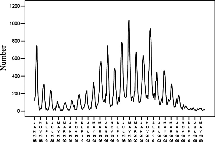
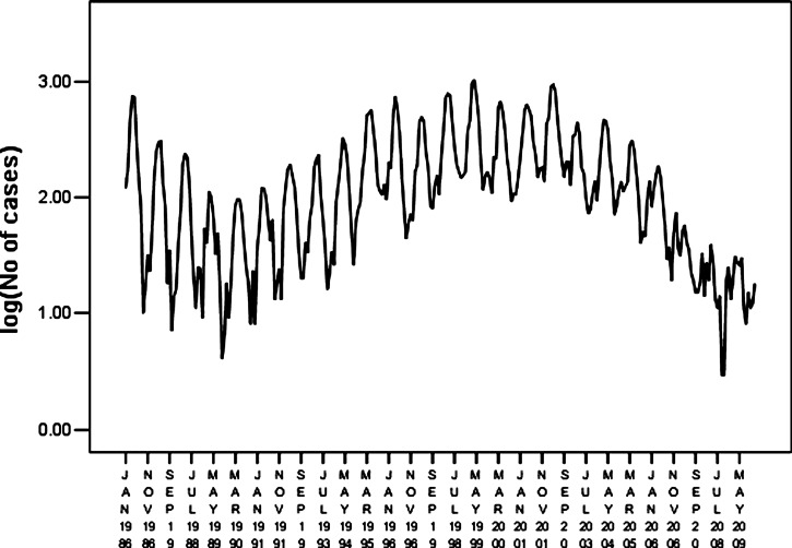
Time series data for HFRS covering 1986–2009 in Hebei Province were used as the training set and monthly data for 2010 were used as the test set (Figure 2). The ARIMA model is based on a stationary time series. A stationary random process should meet the following requirements: the mean and variance should not change over time, and the correlation coefficient should be independent of the time interval but not time. The three types of non-stationary time series have a non-stationary mean, a non-stationary variance, and a periodic or seasonal component.⁸ Because our data had a non-stationary variance (Figure 2), we converted the raw data to its natural logarithm to produce a stationary variance (Figure 3). The converted data series was fitted by linear regression and the regression coefficient was 0.540, which was statistically significant (P = 0.0001). The data series had an upward trend. The sequence diagrams and the seasonal characteristics of HFRS incidence indicated that the data series had a seasonal cycle every 12 months.

Figure 2.

Time series of monthly hemorrhagic fever with renal syndrome cases in Hebei Province, China, during January 1986–December 2009.

Figure 3.

Time series of monthly hemorrhagic fever with renal syndrome cases after natural log transformation in Hebei Province, China, during January 1986–December 2009.

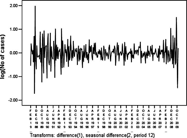
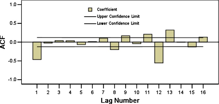
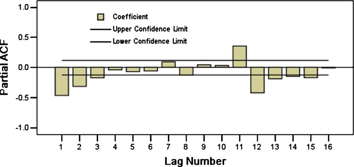
On the basis of these characteristics, we eliminated the effect of seasonal trends (Figure 4) by taking a first-order differential equitation and a seasonal difference equation. The trend of the data series was eliminated (t = −0.038, P = 0.969) and there was no obvious periodicity. This approach yielded a stationary time series. Plausible models, i.e., (the ARIMA (0, 1, 1) × (2, 1, 0)₁₂, ARIMA (0, 1, 1) × (0, 1, 1)_12, and ARIMA (0, 1, 1) × (2, 1, 1)₁₂), were identified on the basis of autocorrelation functions (ACF) and partial autocorrelation functions (PACF) (Figures 5 and 6), and were used for further analysis.

Figure 4.

Time series of monthly hemorrhagic fever with renal syndrome cases after natural log transformation and difference correction in Hebei Province, China, during January 1986–December 2009.

Figure 5.

Autocorrelogram of time series of monthly hemorrhagic fever with renal syndrome cases after natural log transformation and difference correction in Hebei Province, China, during January 1986–December 2009.

Figure 6.

Partial autocorrelogram of time series of monthly hemorrhagic fever with renal syndrome cases after natural log transformation and difference correction in Hebei Province, China, during January 1986–December 2009.

Parameter estimation and model testing.

Model hypothesis testing was conducted on the basis of the P value and Schwarz Bayesian Information Criteria (SBC). The null hypothesis for all parameters coefficients (B) was 0. The goodness of fit statistics were determined by using SPSS, including, the standard error, log-likelihood function values, Akaike information criteria (AIC), and SBC. Smaller AIC values indicate a better model, and the SBC considers the residual error, which is based on AIC. The lowest SBC value with a P value less than 0.05 was considered to be the best model.^9–11 On the basis of parameter estimation and goodness of fit test statistics (Tables 1 and 2), we confirmed that the best model was ARIMA (0, 1, 1) × (2, 1, 0)₁₂.

Table 1.

Parameter estimation for plausible autoregressive integrated moving average (ARIMA) models^*

Parameter	ARIMA (0, 1, 1) × (0, 1, 1)12			ARIMA (0, 1, 1) × (2, 1, 0)12			ARIMA (0, 1, 1) × (2, 1, 1)12
	B	t	P	B	T	P	B	t	P
SAR1	-	-	-	−0.785	−12.344	0.000	−0.652	−4.383	0.000
SAR2	-	-	-	−0.440	−7.200	0.000	−0.366	−3.676	0.000
MA1	0.549	9.596	0.000	0.552	9.715	0.000	0.554	9.742	0.000
SMA1	0.722	12.466	0.000	-	-	-	0.156	0.970	0.333
Constant	0.001	0.430	0.668	0.001	0.365	0.715	0.001	0.396	0.693

^*SAR = seasonal autoregressive parameter; MA = moving average parameter; SMA = seasonal moving average parameter.

Table 2.

Goodness of fit statistics for plausible autoregressive integrated moving average (ARIMA) models^*

Statistic	ARIMA (0, 1, 1) × (0, 1, 1)12	ARIMA (0, 1, 1) × (2, 1, 0)12	ARIMA (0, 1, 1) × (2, 1, 1)12
SE	0.153	0.150	0.150
LL	95.465	99.737	99.874
AIC	−184.930	−191.473	−189.748
SBC	−174.818	−177.991	−172.895

^*SE = standard error; LL = log likelihood; AIC = Akaike information criterion; SBC = Schwarz Bayesian criterion.

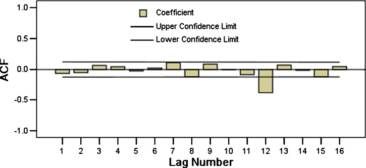
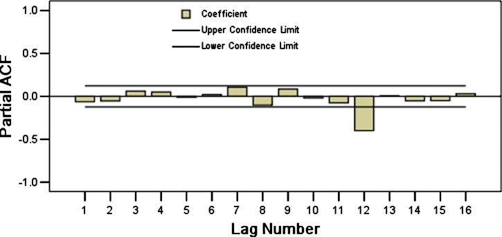
We tested the advantages and disadvantages of the model by comparing the residual error sequences of the original data and the fitted error data series. If the residual was white noise¹² (the data series are of stationary, random, zero related sequences), this finding indicated that the model already contained all the trends found in the original sequence; thus, this model was appropriate for prediction. However, if the residual was not white noise, this indicated that the model should be improved. On the basis of the autocorrelation and partial autocorrelation of the residual errors from the ARIMA (0, 1, 1) × (2, 1, 0)₁₂ model (Figures 7 and 8), the Box-Ljung statistics of the residuals error indicated no significant difference (P > 0.176). The mean of the residual errors was 0.002, indicating no significant difference (P = 0.908). Thus, the residuals error was considered to be white noise sequence, confirming that the selected model was appropriate.

Figure 7.

Autocorrelogram of residual errors for natural logarithm transformation of monthly hemorrhagic fever with renal syndrome cases in Hebei Province, China, during January 1986–December 2009, from the autoregressive integrated moving average (0, 1, 1) × (2, 1, 0)₁₂.

Figure 8.

Partial autocorrelogram of residual errors for natural logarithm transformation of monthly hemorrhagic fever with renal syndrome cases in Hebei Province, China, during January 1986–December 2009, from the autoregressive integrated moving average (0, 1, 1) × (2, 1, 0)₁₂.

Forecast and analysis.

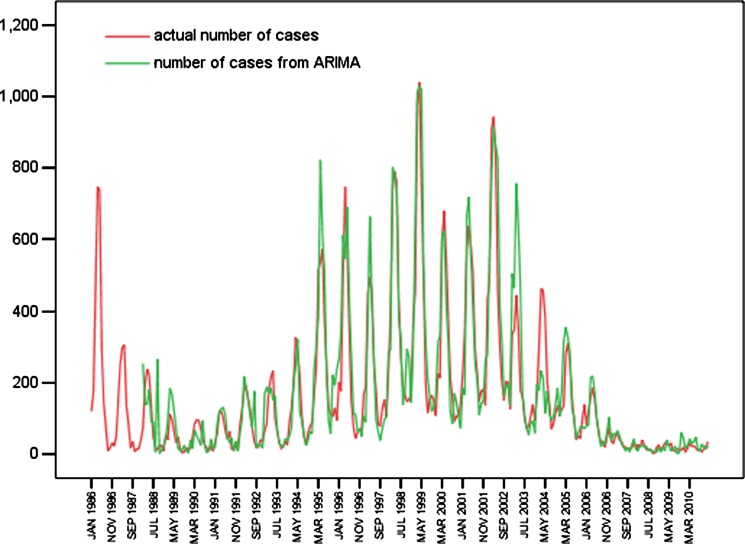
We used ARIMA model (0, 1, 1) × (2, 1, 0)₁₂ and time series data for 1986–2009 as the training set, and we used data from January–December 2010 as the test set (Figure 9, and Table 3). The predicted data for the actual data and the predicted data 95% confidence limit for 2010 are shown in Table 3. The predicted data and the actual data were not perfectly matched, but the actual data fell within the predicted 95% confidence interval.

Figure 9.

Time series of actual number of cases, fitted number of cases, and predicted number of hemorrhagic fever with renal syndrome cases in Hebei Province, China, during January 1986–December 2010.

Table 3.

Comparison of predicted hemorrhagic fever with renal syndrome values and actual values for Hebei Province. China, during January–December 2010^*

No. cases	Jan	Feb	Mar	Apr	May	Jun	Jul	Aug	Sep	Oct	Nov	Dec
Actual value	7	16	32	22	23	17	10	11	7	15	23	35
Predictive value	15	23	42	31	33	48	14	10	29	19	15	24
95% CL of PV	5–47	7–76	12–49	8–117	8–132	11–204	3–63	2–46	6–142	4–100	3–84	4–138

^*CL = confidence level; PV = predicted value.

Discussion

The ARIMA model^13–16 is used widely in medical research and it provides a comprehensive model in the domain of time series analysis. Time series predictions are based on changes over time in historical data sets and they can produce mathematical models by using statistical data that can be extrapolated.¹⁷ Many natural and social environment factors affect the incidence of HFRS, which leads to difficulties when forecasting the incidence of HFRS by using regression forecasting methods. This feature is the main advantage of time series analysis for predicting the incidence of HFRS because time series analysis can consider the effects of various factors. Incidence of HFRS is closely related to rat living habits and the data series indicated significant seasonal changes. The HFRS data series from Hebei Province indicated large fluctuating trends with a cycle of more than 10 years, which was fitted by using ARIMA models. This study also demonstrated the feasibility of HFRS prediction by using ARIMA models.

The seasonal characteristics of HFRS were evident in the ARIMA model, which was modeled on the basis of monthly data. It also forecasted the incident rate monthly. The actual data did not match the predicted data of the model perfectly, but they fell within the predicted 95% confidence interval. There are many reasons for the discrepancies between the actual and predicted data. The model also needs to be modified to consider improved detection methods, large-scale rat elimination, a higher frequency of vaccination, and other factors that will affect the actual incidence.

The prediction accuracy of the ARIMA model was high, but the effect of single-step prediction with the model was much more acceptable than multi-step prediction. This finding might be caused by a better recurrence relationship in the ARIMA model. Single-step forecasts always make predictions on the basis of historical data, whereas multi-step methods make predictions on the basis of values used in second-step modeling. The forecast value error will gradually increase with the recurrence relationships, which reduces the accuracy of multi-step predictions. Because the incidence of HFRS was not stationary, new observations series should be added continually into the sequence over time to ensure that the ARIMA model provides the best forecast possible. If the actual data fall outside the confidence level of the forecast value, the model should be updated immediately. Thus, the ARIMA model is generally used for short-term forecasts.

References

- 1.Zhang YZ, Xiao DL, Wang Y, Wang HX, Sun L, Tao XX, Qu YG. The epidemic characteristics and preventive measures of hemorrhagic fever with syndromes in China. Zhonghua Liu Xing Bing Xue Za Zhi. 2004;25:466–469. [PubMed] [Google Scholar]
- 2.Huaxin C, Chengwang L. Hemorrhagic fever with renal syndrome in China's large-scale application of the vaccine. Zhonghua Liu Xing Bing Xue Za Zhi. 2002;23:145–147. [Google Scholar]
- 3.Li MQ, Liu JJ, Yin K. Discussion on the surveillance and early warning of intestinal infectious diseases in the city outskirts. Dis Surveill. 2006;21:57–58. [Google Scholar]
- 4.Reichert TA, Simonsen L, Sharma A, Pardo SA, Fedson DS, Miller MA. Influenza and the winter increase in mortality in the United States, 1959–1999. Am J Epidemiol. 2004;160:492–502. doi: 10.1093/aje/kwh227. [DOI] [PubMed] [Google Scholar]
- 5.Luz PM, Mendes BV, Codeco CT, Struchiner CJ, Galvani AP. Time series analysis of dengue incidence in Rio de Janeiro, Brazil. Am J Trop Med Hyg. 2008;79:933–939. [PubMed] [Google Scholar]
- 6.Yi J, Du CT, Wang RH, Liu L. Applications of multiple seasonal autoregressive integrated moving average (ARIMA) model on predictive incidence of tuberculosis. Chin J Prev Med. 2007;41:118–121. [PubMed] [Google Scholar]
- 7.Wentong Z. The Course of Statistical Analysis with SPSS. Beijing, China: Hope Electronic Press; 2002. pp. 250–289. [Google Scholar]
- 8.Dunn P. Study Book. Brisbane, Australia: University of Southern Queensland; 2005. [Google Scholar]
- 9.Chafield C. The Analysis of Time Series: Theory and Practice. London: Chapman and Hall; 1975. [Google Scholar]
- 10.Jenkins GW, Reinsel GC. Box GEP. Time Series Analysis. Third edition. South Windor, New South Wales, Australia: Holden Day; 1994. [Google Scholar]
- 11.Bowerman BL, O'Connell R. Forecasting and Time Series: An Applied Approach. Boston: South-Western College Publications; 1987. [Google Scholar]
- 12.Zhang W. SPSS Statistical Analysis Tutorial. Beijing, China: Beijing Electronic Press; 2002. pp. 250–289. [Google Scholar]
- 13.Díaz J, García R, Velázquez de Castro F, Hernández E, López C, Otero A. Effects of extremely hot days on people older than 65 years in Seville (Spain) from 1986 to 1997. Int J Biometeorol. 2002;46:145–149. doi: 10.1007/s00484-002-0129-z. [DOI] [PubMed] [Google Scholar]
- 14.Tingjie L, Xiushen C, Yanfen L. Application of the time-series method to analyze the seasonal distribution of epidemic encephalitis B incidence in Guangdong Province in the years of 1984–1993. Zhonghua Liu Xing Bing Xue Za Zhi. 1998;19:103–106. [PubMed] [Google Scholar]
- 15.Xiaoyong S, Zhiying Z, Dezhong X, Yongping Y, Kaiping C, Yuesheng L, Xiaonong Z. Application of “time series analysis” in the prediction of schistosomiasis prevalence in areas of “breaking dikes or opening sluice for waterstore” in Dongting Lake areas, China. Zhonghua Liu Xing Bing Xue Za Zhi. 2004;25:863–866. [PubMed] [Google Scholar]
- 16.Silawan T, Singhasivanon P, Kaewkungwal J, Nimmanitya S, Suwonkerd W. Temporal patterns and forecast of dengue infection in northeastern Thailand. Southeast Asian J Trop Med Public Health. 2008;39:90–98. [PubMed] [Google Scholar]
- 17.Wen Liang, Xu Dezhong, Lin Minghe, Xia J, Zhang Z, Su Y. Prediction of malaria incidence in malaria epidemic area with time series models. Journal of the Fourth Military Medical University. 2004;25:507–510. [Google Scholar]