Genomic Patterns of Homozygosity in Worldwide Human Populations

Abstract

Genome-wide patterns of homozygosity runs and their variation across individuals provide a valuable and often untapped resource for studying human genetic diversity and evolutionary history. Using genotype data at 577,489 autosomal SNPs, we employed a likelihood-based approach to identify runs of homozygosity (ROH) in 1,839 individuals representing 64 worldwide populations, classifying them by length into three classes—short, intermediate, and long—with a model-based clustering algorithm. For each class, the number and total length of ROH per individual show considerable variation across individuals and populations. The total lengths of short and intermediate ROH per individual increase with the distance of a population from East Africa, in agreement with similar patterns previously observed for locus-wise homozygosity and linkage disequilibrium. By contrast, total lengths of long ROH show large interindividual variations that probably reflect recent inbreeding patterns, with higher values occurring more often in populations with known high frequencies of consanguineous unions. Across the genome, distributions of ROH are not uniform, and they have distinctive continental patterns. ROH frequencies across the genome are correlated with local genomic variables such as recombination rate, as well as with signals of recent positive selection. In addition, long ROH are more frequent in genomic regions harboring genes associated with autosomal-dominant diseases than in regions not implicated in Mendelian diseases. These results provide insight into the way in which homozygosity patterns are produced, and they generate baseline homozygosity patterns that can be used to aid homozygosity mapping of genes associated with recessive diseases.

Introduction

As early as 1876, Charles Darwin reported that inbreeding could lead to reduced fitness in plants.¹ Subsequently, in 1902, Archibald Garrod noted that certain rare traits in humans, such as albinism and alkaptonuria, occurred more frequently in offspring of consanguineous unions.² Recognizing the pattern of recessive inheritance described by Gregor Mendel,³ Garrod attributed his observation to the fact that relatives frequently bear the same inherited gametes, increasing the chance that their offspring will inherit two identical gametes responsible for a recessive trait. In modern terms, an increased recessive-disease incidence in inbred individuals results from the higher probability that they are homozygous for a deleterious recessive allele inherited identically by descent; that is, they are autozygous for the disease allele. This key role of autozygosity in many human diseases has fueled a continued interest in studying the causes and patterns of homozygosity for more than a century.

Population history and cultural factors can affect levels of homozygosity in individual genomes. In some populations, even in the absence of overt inbreeding, homozygosity can be high, because a historical bottleneck or geographic isolation has led to high levels of relatedness among members of a population.^4–8 In other populations, cultural practices that promote consanguineous marriage or endogamy can result in elevated inbreeding levels—and consequently, high levels of homozygosity—even when the overall population size is large.^4,9,10

If individuals inherit the same ancestral mutation identically by descent, then they probably also share adjacent DNA segments on which the mutation first arose. For a recessive phenotype, in affected inbred individuals, the homozygous risk locus therefore probably resides in an unusually long homozygous region. Deleterious recessive variants can thus be identified in affected inbred individuals through detecting long homozygous regions,¹¹ or runs of homozygosity (ROH).¹² This homozygosity-mapping approach¹¹ has enabled the localization of genes associated with recessive Mendelian diseases in hundreds of studies.¹³

Although homozygosity mapping has been focused primarily on inbred affected individuals, recent advances potentially provide a basis for homozygosity mapping in affected individuals who are not inbred.^14–18 Deleterious recessive variants in such individuals might reside in smaller ROH than in inbred individuals, but in ROH nonetheless. Increased density of genotype data has enabled the detection of increasingly smaller ROH, thereby reducing the level of inbreeding required for subjects examined in homozygosity-mapping studies.^14–18 In these studies, however, the fact that patterns of homozygosity, including ROH patterns, are influenced not only by the locations of recessive-disease loci, but also by population history and consanguinity levels, is a major consideration.

Previous studies have found that, in outbred individuals, short ROH that measure tens of kb—the typical range of linkage disequilibrium (LD) in the human genome, and the typical length of a common haplotype that could be paired to form an ROH—are present at high frequencies.¹⁹ Furthermore, ROH of intermediate sizes, measuring hundreds of kb to several Mb, also occur frequently,^{5–7,20–29} probably as a result of background relatedness—recent but unknown kinship among the parents of sampled individuals. Extremely long ROH, measuring tens of Mb, have been observed in as many as 28%–90% of individuals from populations with higher levels of background relatedness;^{4–7,12,24,27} surprisingly, they have also been observed in 2%–26% of individuals in ostensibly outbred populations.^{4,6,7,19–22,24–31} Although some of these long ROH probably reflect recent parental relatedness, others potentially result from a lack of recombination that allows unusually long ancestral segments to persist in the general population.

A high-resolution study of ROH in populations worldwide would provide insight into how population history, cultural practices, and genomic properties could explain the observed patterns of ROH in the human genome. Furthermore, a catalog of the regional variation of ROH across the genome in specific populations would aid the identification of trait-associated ROH in homozygosity-mapping studies. For example, genomic regions that show unusually few ROH might be enriched for loci of critical function or loci harboring lethal or damaging recessive variants. Thus, in homozygosity-mapping studies, disease-associated ROH that occur in regions where ROH are uncommon could be prioritized.

Here, we employ a likelihood-based approach to identify ROH in SNP genotype data from 64 worldwide populations. We classify ROH by length into three groups—short, intermediate, and long—with a model-based clustering algorithm. Next, we investigate the geographic differences in ROH across populations, the genomic distribution of ROH, and its correlation with local genomic features. We show that ROH of different sizes have distinctive continental patterns, both in their total lengths in individual genomes and in their genomic distributions in individual populations, and that these patterns can be explained partly by the properties of recombination and natural selection across the genome. Furthermore, we find that long ROH occur more often in regions associated with autosomal-dominant diseases than in regions not implicated in Mendelian diseases. The results shed new light on the influence of population history and consanguinity on the human genome, and they yield a resource that can ultimately assist in the assessment of homozygosity-mapping signals.

Subjects and Methods

Data Preparation

We examined autosomal SNPs in publicly available phased genotypes for 53 populations in the Human Genome Diversity Panel-CEPH Cell Line Panel^32,33 (HGDP-CEPH panel) and 11 populations in phase III of the International Haplotype Map Project³⁴ (HapMap); SNPs on the mitochondrion and on the X and Y chromosomes were excluded. During the genotype phasing, occasional positions with missing genotypes were imputed (< 0.1% and < 0.2% of all positions in the HGDP-CEPH³² and HapMap³⁴ data sets, respectively); consequently, our data set contains no missing data. We developed a single combined data set after applying quality-control procedures similar to those of Jakobsson et al.³⁵ to eliminate low-quality SNPs.

HGDP-CEPH

We used 938 individuals from the H952 subset,³⁶ in which no pair of individuals is more closely related than first cousins, considering phased genotypes for the individuals studied by Li et al.³² at 640,698 autosomal SNPs.³³ After quality control (Figure S1 available online), the final data set contained 640,034 SNPs; 664 SNPs were excluded because of Hardy-Weinberg disequilibrium in at least one of two groups with low levels of population structure:³⁵ a Middle Eastern group consisting of Bedouin, Druze, and Palestinian samples (133 individuals), and a sub-Saharan African group consisting of Bantu (southern Africa), Bantu (Kenya), Mandenka, and Yoruba samples (62 individuals). We performed Yates-corrected chi-square tests³⁷ of Hardy-Weinberg equilibrium in each of the groups, using the same exclusion criteria as in Jakobsson et al.³⁵

HapMap

The HapMap Phase III data set³⁴ (release 2, downloaded May 3^rd, 2009) consisted of 993 individuals, for whom phased genotypes were available at 1,387,216 autosomal SNPs. We considered 901 unrelated individuals from the HAP1117 subset,³⁸ in which no pair is more closely related than first cousins. After quality control (Figure S1), the final data set contained 1,361,534 SNPs. One SNP that was triallelic (rs1078890) and 539 SNPs that were monomorphic in the 901 individuals were removed. A further 25,142 SNPs were excluded because of Hardy-Weinberg disequilibrium in at least one of the 11 HapMap populations: we performed Yates-corrected chi-square tests of Hardy-Weinberg equilibrium in each population,³⁷ using the same exclusion criteria as in Pemberton et al.³⁸

Combined Data

We assembled a data set containing 1,839 individuals (938 HGDP-CEPH, 901 HapMap) from 64 populations (Table S1; mean sample size = 28.7, SD = 27.4) and 577,489 SNPs that the two data sets shared in common. At 17,970 SNPs, the data sets had genotypes given for opposite strands, and we converted the HapMap genotypes to match the HGDP-CEPH genotypes.

Geographic Locations

Some analyses required the geographic coordinates of the populations. Geographic distances from Addis Ababa, Ethiopia (9°N, 38°E) were calculated as in Rosenberg et al.³⁹ with the use of waypoint routes, taking HGDP-CEPH locations from Cann et al.⁴⁰ For the HapMap GIH (Gujarati Indians in Houston, Texas) population we adopted the location used for Gujaratis by Rosenberg et al.⁴¹ Actual sampling locations were used for the HapMap LWK (Luhya in Webuye, Kenya) (0°N, 34°E) and MKK (Maasai in Kinyawa, Kenya) (0°N, 37°E) populations. For the HapMap TSI (Toscani in Italy), YRI (Yoruba in Ibadan, Nigeria), JPT (Japanese in Tokyo), CHB (Han Chinese in Beijing), and CHD (Chinese in Metropolitan Denver, Colorado) populations, we used the coordinates of the HGDP-CEPH Tuscan, Yoruba, Japanese, and Han Chinese populations, respectively. Admixed populations ASW (African ancestry in Southwest USA) and MXL (Mexican ancestry in Los Angeles, California) were omitted from geographic analyses, as was the geographically imprecise CEU (Utah residents of Northern and Western European ancestry) group.

Identification of ROH

To identify ROH, we adapted the method of Wang et al.⁴² that is based on the earlier method of Broman and Weber.¹² In brief, for each individual and for a sliding window of a fixed number (n) of SNPs, incremented by m SNPs along a chromosome, in each window we calculated the LOD of autozygosity, defined as the base-10 logarithm of the ratio of the probabilities of the genotype data under hypotheses of autozygosity and nonautozygosity. The probabilities incorporate population-specific allele-frequency estimates and an assumed rate ε of genotyping errors (and mutations).

To adjust for sample-size differences among populations, we used a resampling procedure to estimate the allele frequencies used in the LOD score calculation.³⁵ For each population, at each SNP, we sampled 40 nonmissing alleles with replacement and calculated the allele frequencies from these 40 alleles; in each population, resampling was performed independently across SNPs. As a consequence of the resampling procedure, it was possible for an individual to possess an allelic type whose frequency was estimated to be 0 in the sample of 40 alleles used to calculate allele frequencies. SNP positions at which this scenario was encountered were treated as missing when calculating the LOD scores for all windows containing the positions in individuals that had the allelic type of frequency 0 (i.e., the multiplicative contribution of the position to the likelihood ratio was set to 1). We encountered this situation in only 0.23% of windows across all individuals in our data set, and in at most 1.22% of windows in a given individual (mean = 0.23%, SD = 0.13%). Considering all windows in all individuals, at most seven instances occurred among the SNPs in a given window (mean = 0.002 instances, SD = 0.053).

We set the window increment m to 1 SNP and the genotyping error rate ε to 0.001, a conservative value that is similar to but slightly higher than the rate of genotype discrepancy for duplicate samples.³⁵ We investigated window widths (n) of 20, 30, 40, 50, 60, 70, 80, 90, and 100; n = 60 was the largest value that produced a clear bimodal LOD score distribution in all populations (data not shown), and it was therefore chosen. Whereas Wang et al. compared the LOD scores of two groups of individuals for the purpose of identifying windows that differed in homozygosity levels between the groups,⁴² we sought to use the LOD scores to infer the homozygosity status of the windows in each individual. In each population we therefore defined a LOD-score threshold, above which a window was called as a homozygosity run. Modes differed across populations, and for a given population, the threshold was chosen as the local minimum between the two LOD modes (Table S1). In identifying these minima, we used Gaussian kernel density estimates of the genome-wide LOD-score distributions (Figure 1). Contiguous windows that exceeded the population-specific LOD-score threshold were joined and considered to be a single ROH. To evaluate the relationship of LOD-score threshold with geographic distance from Addis Ababa, an approximate location for the origin of out-of-Africa migration, we calculated the coefficient of determination (R²) for the regression of the LOD-score threshold on geographic distance, using lm in R⁴³ (from the stats package, as with all subsequent R functions, unless specified otherwise).

Figure 1.

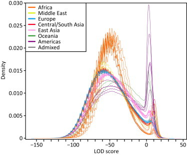
LOD-Score Distributions in 64 Populations

Each line represents the Gaussian kernel density estimates of the pooled LOD scores from all individuals in a given population, colored by geographic affiliation. The ASW and MXL admixed populations appear in gray. The periodicity of each density is a consequence of the resampling approach used to estimate allele frequencies.

Size Classification of ROH

Separately in each population, we modeled the distribution of ROH lengths as a mixture of three Gaussian distributions that we interpreted as representing three ROH classes: (A) short ROH measuring tens of kb that probably reflect homozygosity for ancient haplotypes that contribute to local LD patterns, (B) intermediate ROH measuring hundreds of kb to several Mb that probably result from background relatedness owing to limited population size, and (C) long ROH measuring multiple Mb that probably result from recent parental relatedness. We ran unsupervised three-component Gaussian fitting of the ROH length distribution, using Mclust from the mclust package (v.3) in R, and allowing component magnitudes, means, and variances to be free parameters (Figure 2A). Models with two to ten components were investigated, and only for the three-component model was it possible in each population to partition the real number line into disjoint intervals equal in number to the number of components, such that each interval contained ROH only in one of the components (Figure 2B). For each population, denoting the minimum and maximum ROH sizes in classes A, B, and C (ordered from smallest to largest) by A_min and A_max, B_min and B_max, and C_min and C_max, we defined the size boundaries between classes A and B and classes B and C as (A_max + B_min)/2 and (B_max + C_min)/2. Across all populations, A-B boundaries lay in [379,554 bp; 679,619 bp], with a mean of 509,618 bp and SD of 60,183 bp (Table S1). B-C boundaries lay in [896,699 bp; 2,191,780 bp], with a mean of 1,548,382 bp and SD of 303,986 bp (Table S1). To compare per-individual total lengths of ROH across classes, we used cor.test in R to calculate the Pearson correlation coefficient (r) between total lengths in different pairs of classes, considering all individual genomes. Violin plots⁴⁴ of total lengths and total numbers of ROH in individual genomes were produced using vioplot from the vioplot package in R.

Figure 2.

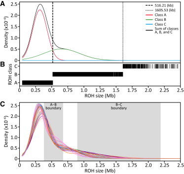
Classification of ROH into Three Size Classes

(A) An example Gaussian kernel density estimation of the ROH size distribution in a single population (French), with the boundary between ROH classes A and B marked by the vertical dashed line (0.516 Mb) and the boundary between classes B and C marked by the vertical dotted line (1.606 Mb).

(B) Inferred assignment of ROH into the three classes for the French population. Only ROH less than 2.5 Mb in length are shown. However, all ROH, regardless of length, were used in the analysis.

(C) Gaussian kernel density estimates of the ROH size distribution in each of the 64 populations, where each line represents a different population, colored by geographic affiliation (Figure 1). The size ranges across the 64 populations of the boundaries between ROH classes A and B and between classes B and C are shown by the shaded boxes.

Geographic Pattern of ROH

To compare the genomic distribution of ROH across populations, we performed classical (metric) multidimensional scaling (MDS). First, for each size class, in each population, at each SNP, we calculated the proportion of individuals from the population that had an ROH that included the SNP (the ROH frequency, Tables S2, S3, and S4). In a sample of N individuals, the proportion p_x of individuals with an ROH of class x (x∈{A,B,C}) at SNP k was calculated as

$$p_x=\frac{n_x}{N-n_{x^{\prime }}},$$ (Equation 1)

where n_x is the number of individuals with an ROH of class x that included SNP k, and n_x′ is the number of individuals with an ROH in one of the remaining classes ({A,B,C}\{x}) that included SNP k. In rare cases with n_x′ = N (i.e., all individuals were covered by one or both of the other classes, and none could have carried a run of class x), we set p_x to “missing” (instead of 0).

For each ROH size class and each pair of populations, we calculated ROH similarity between populations as the Pearson correlation coefficient (r) of their SNP-wise ROH frequencies. We then applied MDS to the similarity matrix using cmdscale in R. For each class, to compare the MDS plot with that previously obtained for 29 HGDP-CEPH populations from SNP genotypes,⁴⁵ using the method of Wang et al.,⁴⁵ we computed the Procrustes similarity t₀ between the 29-population SNP-based MDS plot of Wang et al. and the restriction of our MDS plot to the 29 populations. The significance of t₀ estimates under the null hypothesis of no similarity between plots was evaluated with 10,000 permutations of population labels.

Genomic Distribution of ROH

To study the spatial distribution of ROH across the genome, we calculated SNP-wise ROH frequencies, considering all sampled individuals and jointly considering all three size classes (Table S5). In a sample of N individuals, the frequency p_all of individuals with an ROH of any size class at SNP k is

$$p_{all}=\frac{n_{all}}{N},$$ (Equation 2)

where n_all is the number of individuals with an ROH in any class. Next, we defined as ROH hotspot locations where p_all exceeded 30.34%, the 99.5^th percentile among all p_all values. We ranked ROH hotspots by the mean ROH frequency across the SNPs they contained. In rare cases in which multiple hotspots had the same mean frequency, we broke ties with the maximum ROH frequency across SNPs within hotspots. Similarly, we defined ROH coldspots as locations in which p_all was less than 2.72%, the 0.5^th percentile among values of p_all, ranking them as in the analysis of hotspots. In cases of ties in mean frequency for coldspots, the one with the lowest minimum ROH frequency was ranked as a stronger coldspot. Because less information is available for identification of ROH at chromosome ends, we ignored the first and last 60 SNPs on each chromosome arm when identifying hotspots and coldspots.

To investigate whether the number of ROH hotspots per chromosome differed significantly from the number of ROH coldspots, we compared the numbers of ROH hotspots and coldspots on each chromosome using a Wilcoxon signed-rank test, performed with wilcox.test in R.

To study how ROH hotspots and coldspots varied across geographic regions, we calculated SNP-wise ROH frequencies separately in each geographic region using Equation 2, jointly considering all three ROH size classes (Table S5). We then identified hotspots and coldspots separately in each region using the same method as was used in the full data set.

Relationship between ROH and Genomic Variables

For each ROH size class, we investigated recombination rate and integrated haplotype scores⁴⁶ (iHS) for correlations with ROH frequency (Equation 1) across the genome. Population-based recombination-rate estimates were obtained from release 22 of HapMap Phase II (downloaded January 30^th, 2009).¹⁹ iHS values for each of the 53 HGDP-CEPH populations were obtained from the HGDP Selection Browser (downloaded December 1^st, 2011).³³

Because the density of available data points differed for recombination rate, iHS, and ROH frequency, we summarized these variables over nonoverlapping windows of w bases, excluding windows within centromeres. We defined w separately for each ROH class as the minimum ROH size of that class: A, w = 34,129 bp; B, w = 379,565 bp; C, w = 897,801 bp. We then calculated for each window the mean ROH frequency across SNPs in the window and the mean recombination rate across all data points within the window for which a recombination rate was available. Similarly, separately in each of the 53 HGDP-CEPH populations, we calculated for each window the mean iHS across all data points available for iHS within the window. In rare cases of no data points available within a window, we omitted the window in subsequent computations. Thus, for each ROH class, we obtained a vector of mean ROH frequencies equal in length to the number of windows and similar vectors of mean recombination rate and iHS.

Separately for each ROH class, we calculated the Spearman’s rank correlation coefficient (ρ) between ROH frequency and recombination rate using cor.test in R. To display the two-way distribution of ROH frequency and recombination rate, we partitioned their bivariate combinations into a 100 × 100 square grid, and using image from the spam package in R, we plotted the counts in the grid as a heat map. To remove the potential confounding effect of recombination rate when evaluating the relationship between ROH frequency and iHS, we performed partial-correlation analyses using pcor.test⁴⁷ in R. Separately for each ROH class, in each HGDP-CEPH population, we calculated the Spearman’s partial rank correlation coefficient $\left({\rho }_{pc}\right)$ between ROH frequency and iHS, including recombination rate as a covariate. To evaluate the relationship of ${\rho }_{pc}$ with geographic distance from Addis Ababa, separately for each ROH class, we calculated the coefficient of determination (R²) for the regression of ${\rho }_{pc}$ on geographic distance. We then investigated differences in ${\rho }_{pc}$ between ROH classes, separately for all three pairs of classes, by comparing paired lists of the 53 population-level ${\rho }_{pc}$ values using a Wilcoxon signed-rank test.

To compare ROH frequencies between genes associated with autosomal-recessive diseases, autosomal-dominant diseases, and neither type of disease, we used the hg18 release of the UCSC gene database to define genic regions (i.e., the transcribed region of a gene). Overlapping genic regions were merged, creating 16,721 nonoverlapping regions. For each ROH class, we calculated the mean ROH frequency across SNPs in each genic region, ignoring the 2,781 genic regions that had no genotyped SNPs. Because genome-wide patterns in ROH frequency showed significant correlations with recombination rate (see Results), we recombination-adjusted ROH frequency before comparing its distribution between recessive, dominant, and non-OMIM genic regions. First, in each of the 13,940 genic regions for which we could calculate a mean ROH frequency, we calculated the mean recombination rate across available data points, ignoring one genic region that had no data points available for recombination rate within the region. Second, we ran a locally weighted linear regression of ROH frequency against recombination rate with the model $F_k={\beta }_0+{\beta }_r{R}_k+{\epsilon }_k$ using loessFit from the limma package in R, where ${\beta }_0$ is the intercept, ${\beta }_r$ is the regression coefficient, and $F_k$ and ${\epsilon }_k$ are the ROH frequency and error term of region k, respectively. To ensure constant variance of the error term, we used log_e-transformed recombination rates as $R_k$. Third, using the Online Mendelian Inheritance in Man (OMIM) database (accessed May 24, 2010), we identified 699 genic regions associated only with autosomal-recessive diseases (and not with dominant diseases) and 515 genic regions associated only with autosomal-dominant diseases (and not with recessive diseases) for which regression residuals were available. For comparison, we used 12,491 autosomal genic regions that have not been associated in OMIM with either recessive or dominant diseases (non-OMIM genic regions) and for which regression residuals were available; 234 genic regions associated with both recessive and dominant diseases were not considered. We then compared the distributions of regression residuals among recessive genes, dominant genes, and non-OMIM genes using two-sided Kolmogorov-Smirnov (KS) tests (ks.test in R).

Results

Identification and Size Classification of ROH

We used a likelihood approach to identify ROH in genotype data for 1,839 unrelated individuals that represent 64 worldwide populations. For a given 60-SNP window, the probabilities of observing the genotype data under the hypothesis of autozygosity and under the null hypothesis of nonautozygosity were compared in a LOD score. The distribution of LOD scores for all windows in the genome is bimodal (Figure 1), with population-dependent modes and a noticeable shift toward lower LOD scores in non-African populations. LOD scores on the left-hand side favor the hypothesis of nonautozygosity, whereas those on the right-hand side favor the autozygosity hypothesis. The bimodal distribution therefore provides evidence for the presence of genomic regions of autozygosity. As the area under the right-hand mode is greater in populations at a greater distance from Africa, it suggests that autozygous regions are more frequent in these populations.

We defined LOD-score thresholds above which a genomic window is considered an ROH. For a given population, the threshold can be naturally placed at the minimum between the two modes for the population, and for the rest of this study, we refer to windows with LOD scores above the threshold as ROH; consecutive ROH windows are joined. The population-specific thresholds (Table S1) are negatively correlated with geographic distance from East Africa, as measured with great-circle distance from Addis Ababa via land-based routes (R² = 0.757; Figure S2). This correlation is similar to the negative correlation observed for expected heterozygosity.^32,48,49

In each population, the size distribution of ROH appears to contain multiple components (Figure 2A). Using a three-component Gaussian mixture model, we classified ROH in each population into three size classes (Figure 2B): short (class A), intermediate (class B), and long (class C). Size boundaries between different classes vary across populations (Table S1); however, considering all populations, all A-B boundaries are strictly smaller than all B-C boundaries (Figure 2C). The mean sizes of class A and B ROH are similar among populations from the same geographic region (Figure S3), with the exception that Africa and East Asia have greater variability. The class C mean is generally largest in the Middle East, Central/South Asia, and the Americas and smallest in East Asia (Figure S3), with the exception that the Tujia population has the largest value. In the admixed Mexican population (MXL), mean ROH sizes are similar to those in European populations. In the admixed African American population (ASW), however, mean ROH sizes are among the smallest in our data set, notably smaller than in most Africans and Europeans.

Geographic Pattern of ROH

Several patterns emerge from a comparison of the per-individual total lengths of ROH across populations (Figure 3). First, the total lengths of class A (Figure 3A) and class B (Figure 3B) ROH generally increase with distance from Africa, rising in a stepwise fashion in successive continental groups. This trend is similar to the observed reduction in haplotype diversity with increasing distance from Africa.^32,35,50,51 Second, total lengths of class C ROH (Figure 3C) do not show the stepwise increase. Instead, they are higher and more variable in most populations from the Middle East, Central/South Asia, Oceania, and the Americas than in most populations from Africa, Europe, and East Asia. This pattern suggests that a larger fraction of individuals from the Middle East, Central/South Asia, Oceania, and the Americas tend to have higher levels of parental relatedness, in accordance with demographic estimates of high levels of consanguineous marriage particularly in populations from the Middle East and Central/South Asia,^52,53 and it is similar to that observed for inbreeding-coefficient⁵⁴ and identity-by-descent⁵⁵ estimates. Third, in the admixed ASW and MXL individuals, total lengths of ROH in each size class are similar to those observed in populations from Africa and Europe, respectively (Figure 3).

Figure 3.

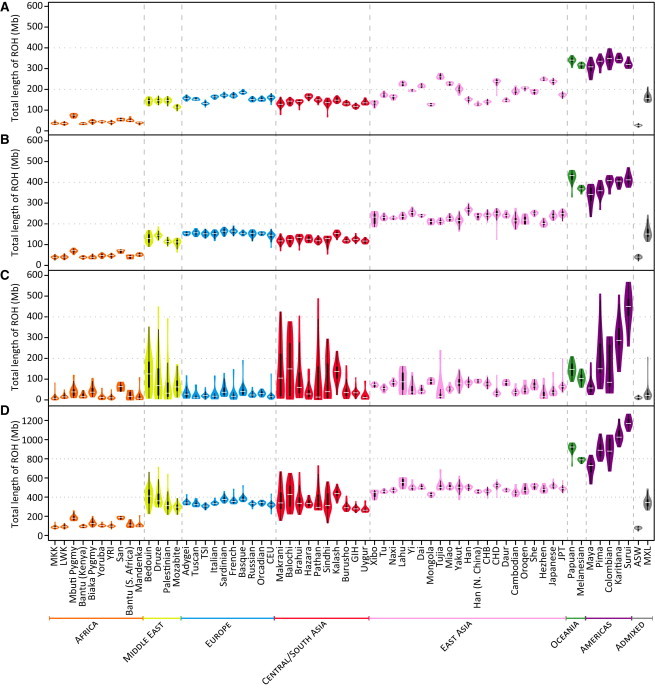
Population-Specific Distributions of the Total Length of ROH per Individual

Data are shown as “violin plots,” representing the distribution of total ROH length over all individuals in each of the 53 HGDP-CEPH and 11 HapMap populations, for (A) class A, (B) class B, (C) class C, and (D) all three classes combined. Each “violin” contains a vertical black line (25%–75% range) and a horizontal white line (median), with the width depicting a 90°-rotated kernel density trace and its reflection, both colored by the geographic affiliation of the population.⁴⁴ Populations are ordered from left to right by geographic region and within each region by increasing geographic distance from Addis Ababa.

The total numbers of ROH per individual (Figure S4) show similar patterns to those observed for total lengths (Figure 3). However, in East Asian populations, total numbers of class B and class C ROH per individual are notably more variable across populations than are ROH total lengths.

Correlations among ROH Size Classes

To quantitatively assess the patterns observed in the population-level distributions of total ROH length in Figure 3, we performed pairwise comparisons between the total lengths of class A, class B, and class C ROH in individual genomes (Figure 4). As implied by Figure 3, the total lengths of class A and B ROH are highly correlated (r = 0.899, p < 10⁻¹⁶). Neither is strongly correlated with the total length of class C ROH (r = 0.381 with p < 10⁻¹⁶ and r = 0.410 with p < 10⁻¹⁶, respectively), however, suggesting that class C and class A and B ROH may have arisen via different processes: class C from recent inbreeding, and class A and B ROH from population-level LD patterns on different evolutionary scales.

Figure 4.

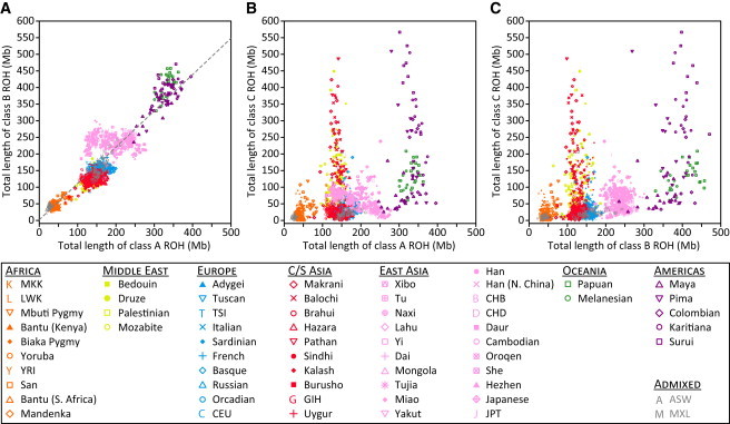
Comparison of per-Individual Total ROH Lengths across Size Classes

(A) Class B versus class A (r = 0.899, p < 10⁻¹⁶).

(B) Class C versus class A (r = 0.381, p < 10⁻¹⁶).

(C) Class C versus class B (r = 0.410, p < 10⁻¹⁶).

Genomic Distribution of ROH

For the different size classes, the distributions of ROH across the genome are largely nonuniform. As an example, Figure 5 shows the distribution of ROH frequencies on chromosome 3 for each of the 64 populations analyzed. In agreement with the patterns observed for total ROH lengths per individual, ROH frequencies for each class increase progressively through populations from Africa, the Middle East, Europe, Central/South Asia, and East Asia to Oceania and the Americas. The nonuniform patterns of ROH across the chromosome vary among populations, especially for class C, and to a lesser extent, for class B.

Figure 5.

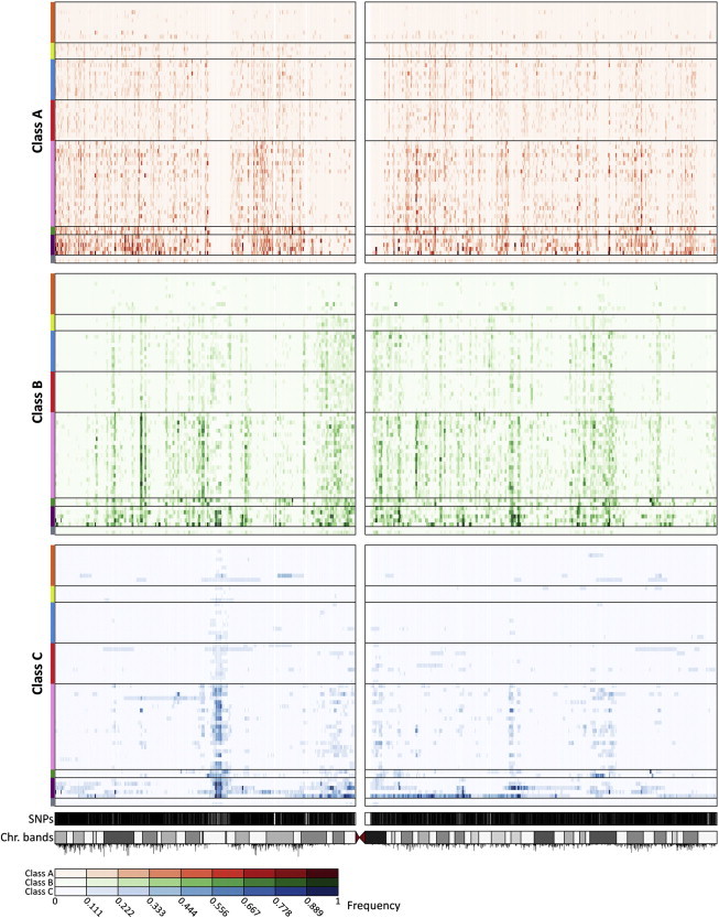
Distribution of ROH Frequency across Chromosome 3 for Each ROH Class

For each ROH class, for each population, at each SNP, the proportion of individuals in that population who have an ROH encompassing the SNP is plotted. Each row represents a population, and each column represents a genotyped SNP position. The intensity of a point increases with increasing ROH frequency, as indicated by the color scale below the figure. Populations are ordered from top to bottom by geographic affiliation, as indicated by colored bars on the left, and within regions from top to bottom by increasing geographic distance from Addis Ababa (in the same order as in Figure 3). SNP positions and the ideogram of chromosome banding are in the bottom tracks. Recombination rates are represented by vertical black lines below the ideogram, with line heights proportional to recombination rates.

MDS plots on the basis of the genomic distributions of class A (Figure 6A) and class B (Figure 6B) ROH frequencies are similar to a previous MDS plot on the basis of SNP genotypes,⁴⁵ grouping the populations by geographic region (Procrustes similarity t₀ = 0.946 for class A, p < 0.001; t₀ = 0.910 for class B, p < 0.001). By contrast, the MDS plot for class C ROH (Figure 6C) matches the SNP-level plot less closely (t₀ = 0.778, p < 0.001); the populations fall into two loose clusters, one for populations from Africa, the Middle East, Europe, and Central/South Asia, and the other for those from East Asia, Oceania, and the Americas. These observations are consistent with the interpretation that class A and B ROH, for which neighboring populations have similar patterns, reflect long-term aspects of population structure that have affected population similarity at the SNP level, and that class C ROH, for which neighboring populations do not necessarily have similar patterns, reflect a different and more recent phenomenon.

Figure 6.

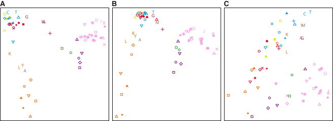
Geographic Groupings in the Distribution of ROH Frequencies across the Genome

The first two dimensions of a multidimensional scaling analysis of pairwise correlations between genome-wide ROH frequencies in individual populations are shown for: (A) class A, (B) class B, and (C) class C ROH. Populations are indicated by the same symbols as in Figure 4.

Hotspots and Coldspots of ROH

The nonuniform patterns of ROH across the genome (Figure 7) uncover regions where ROH are unusually frequent (hotspots) or infrequent (coldspots). ROH hotspots are regions with reduced diversity—and thus increased homozygosity—compared to the rest of the genome, whereas ROH coldspots are regions with increased diversity. The existence of ROH hotspots and coldspots can be explained partly as a consequence of stochasticity in recombination events across the genome or variation across the genome in the effects of demographic processes influencing genetic diversity. However, ROH hotspots could also represent regions that harbor targets of positive selection and that have experienced an overall reduction in genetic diversity and an increase in homozygosity around selected loci.

Figure 7.

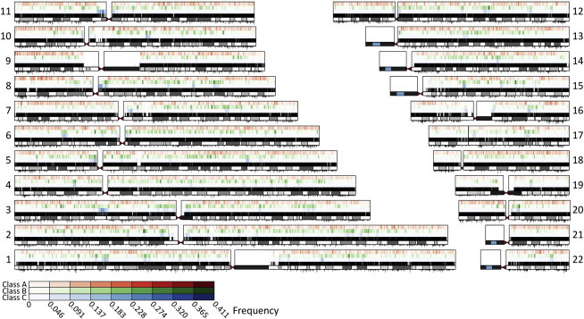
Distribution of Worldwide Mean ROH Frequency across the Genome

For each chromosome, the figure shows the ROH frequency for class A (top), class B (middle), and class C (bottom). SNP position, chromosome banding, and recombination rates are shown as in Figure 5.

To further investigate the properties of ROH hotspots and coldspots, we focused on regions of the genome that contained SNPs in the extreme tails (< 0.5% or > 99.5%) of the empirical distribution of total ROH frequencies calculated over all three size classes and over all populations (Table S5). All SNPs with ROH frequencies above the 99.5^th percentile fall in 69 genomic regions declared to be ROH hotspots, and all SNPs below the 0.5^th percentile lie in 65 ROH coldspots. The distribution of the number of ROH hotspots across autosomes does not differ significantly from the distribution of the number of ROH coldspots (p = 0.965, Wilcoxon signed-rank test).

ROH Hotspots

The top ten hotspots—the regions with the highest frequencies of ROH—appear in Table 1. They range in size from 400 kb to nearly 1 Mb, and each is carried by 34% to 43% of individuals. The top-ranked ROH hotspot is located on chromosome 2p in a region that has low recombination rates (Figure S5A) and that contains the exocyst complex component gene, EXOC6B (Figure S5B). In this region, ROH frequencies are highest in East Asians and lowest in Africans (Figure S5C). The gene contains 24 near-fixed differences between East Asians and Africans,⁵⁶ and the region surrounding EXOC6B has been identified as a strong candidate for recent positive selection in East Asians.^57,58

Table 1.

The Top Ten ROH Hotspots on Human Autosomes

Rank	Chr	Genomic Region (kb)			ROH Frequency			Content
		Begin	End	Length	Max	Mean	SD	miRNA	RefSeq Genes
1a	2	72,209	72,982	773	0.458	0.427	0.034	−	CYP26B1, EXOC6B, SPR
2	20	33,546	34,281	735	0.410	0.372	0.037	−	C20orf173, C20orf152, CEP250, CPNE1, EPB41L1, ERGIC3, FER1L4, LOC647979, NFS1, PHF20, RBM12, RBM39, ROMO1, SCAND1, SPAG4
3a	1	103,134	103,530	396	0.411	0.370	0.030	−	COL11A1b
4	9	125,357	125,762	405	0.394	0.367	0.023	−	DENND1A
5	10	73,578	74,430	852	0.384	0.362	0.021	−	ANAPC16, ASCC1, CBARA1, CCDC109A, DDIT4, DNAJB12, OIT3, PLA2G12B
6a	3	25,703	26,273	569	0.379	0.359	0.011	−	LOC285326, NGLY1, OXSM
7	5	44,604	45,448	843	0.393	0.355	0.023	−	HCN1, MRPS30
8	15	69,881	70,571	690	0.367	0.347	0.011	−	ARIH1, C15orf34, CELF6, GRAMD2, HEXA,cMYO9A, NR2E3, PARP6, PKM2, SENP8, TMEM202
9a	12	86,938	87,756	818	0.388	0.344	0.033	−	C12orf29, C12orf50, CEP290,dKITLG,eTMTC3
10a	4	33,305	34,259	954	0.378	0.343	0.018	−	−

The following abbreviations are used: Chr, chromosome; ROH, runs of homozygosity; Max, maximum; and miRNA, microRNA. Regions are ordered from top to bottom by decreasing worldwide mean ROH frequency. Genes in bold and underlined are associated with autosomal-dominant and autosomal-recessive diseases, respectively, in the OMIM database.

^aThese hotspots overlap regions identified in previous genomic surveys as probable targets of recent positive selection.^33,57,59,60

^bStickler syndrome (MIM 604481) and Marshall syndrome (MIM 154780).

^cTay-Sachs disease (MIM 272800).

^dSenior-Loken syndrome (MIM 610819), Joubert syndrome (MIM 610188), Leber congenital amaurosis (MIM 611755), Meckel syndrome (MIM 611134), and Bardet-Biedel syndrome (MIM 209900).

^eFamilial progressive hyperpigmentation (MIM 145250).

Among the next nine top hotspots, four have been identified in previous genomic surveys as probable targets of recent positive selection.^33,57,59,60 For example, the third-ranked hotspot, which has a pronounced elevation in ROH frequencies primarily in East Asians (data not shown), lies in a region reported to have undergone positive selection in populations of Chinese descent.⁵⁹ This region contains COL11A2, a gene essential for cartilage-tissue development⁶¹ and implicated in Stickler syndrome type III⁶² and Marshall syndrome.⁶³ The ninth-ranked hotspot lies in a region reported to have undergone positive selection in non-Africans^33,59,60,64 and has higher ROH frequencies in non-Africans than in Africans (data not shown). This region contains KITLG (Table 1), a determinant of human skin pigmentation.^64,65

In separate analyses for each geographic region, the location of the top-ranked hotspot varies across continental regions (Table S6). Of these geographic-region-specific top-ranked hotspots, three lie in genomic regions that have been identified as probable targets of recent positive selection in their respective geographic regions.^33,57,59,60 We observed that ROH frequencies in some hotspots varied greatly across geographic regions. For example, the top-ranked hotspot in Oceania lies on chromosome 8p, in a genomic region that has a nontrivial recombination rate (Figure S6A) and contains only two genes (Figure S6B). This region was reported as a selection target in Oceanians.³³ Whereas at most SNPs in this region, > 85% of the Oceanians were homozygous, none of the other geographic regions had > 31% homozygous individuals at any SNP in the region (Figure S6C).

ROH Coldspots

The top ten ROH coldspots appear in Table 2. They range in size from 88 kb to 1.41 Mb, and each is carried by only 1.47% to 1.90% of individuals. The top-ranked coldspot lies on chromosome 3q in a region that has high recombination rates (Figure S7A) and contains five genes (Figure S7B). In this region, ROH frequencies are lowest in Oceanians and highest in Native Americans (Figure S7C). Of the next nine top coldspots, the fifth-ranked coldspot contains the largest known microRNA gene cluster in the human genome (C19MC), a primate-specific cluster of tandemly repeated microRNA genes that underwent a rapid Alu-mediated expansion during primate evolution.^66,67

Table 2.

The Top Ten ROH Coldspots on Human Autosomes

Rank	Chr	Genomic Region (kb)			ROH Frequency			Content
		Begin	End	Length	Min	Mean	SD	miRNA	RefSeq Genes
1	3	195,095	195,561	466	0.015	0.019	0.004	−	CPN2, HES1, LRRC15, LOC100128023, LOC100131551
2	19	540	1,949	1,409	0.016	0.019	0.003	MIR3187, MIR1909	ABCA7, ADAMTSL5, ADAT3, APC2, ARID3A, ATP5D, ATP8B3, AZU1, BTBD, C19orf6, C19orf21, C19orf22, C19orf23, C19orf24, C19orf25, C19orf26, C19orf34, CFD,aCIRBP, CNN2, CSNK1G2, DAZAP1, EFNA2, ELANE, FAM108A1, FGF22, FSTL3, GAMT,bGPX4, GRIN3B, HCN2, HMHA1, KISS1R,cKLF16, LOC100288123, LPPR3, MBD3, MED16, MEX3D, MIDN, MUM1, NDUFS7,dONECUT3, PALM, PCSK4, PLK5P, POLR2E, POLRMT, PRSSL1, PRTN3, PTBP1, REEP6, REXO1, RNF126, RPS15, SBN02, SCAMP4, STK11,eTCF3, UQCR11, WDR18
3	10	131,492	131,693	200	0.017	0.020	0.002	MIR4297	EBF3
4	18	69,604	69,722	118	0.017	0.020	0.003	−	−
5	19	58,569	59,6067	1,036	0.015	0.021	0.003	C19MC, MIR371, MIR372, MIR373, MIR935	CACNG6, CACNG7, CACNG8, CNOT3, DPRX, LAIR1, LENG1, LILRA3, LILRA4, LILRA5, LILRA6, LILRB2, LILRB3, LILRB5, LOC284379, MBOAT7, MYADM, NDUFA3, NLRP12, OSCAR, PRKCG,fPRPF31,gRPS9, TARM1, TFPT, TMC4, TSEN34, VSTM1, ZNF331, ZNF525, ZNF761, ZNF765, ZNF813
6	6	41,512	41,719	207	0.016	0.021	0.003	−	FOXP4, MDFI
7	16	77,531	77,621	90	0.019	0.022	0.002	−	WWOX
8	19	2,959	3,743	785	0.016	0.022	0.004	−	AES, APBA3, C19orf28, C19orf29, C19orf71, C19orf77, CELF5, DOHH, FZR1, GIPC3, GNA11, GNA15, HMG20B, MATK, MRPL54, NCLN, NFIC, PIP5K1C, RAX2, S1PR4, TBXA2R, TJP3, TLE2
9	19	61,317	61,444	127	0.021	0.022	0.002	−	GALP, ZNF444, ZNF787, ZSCAN5A, ZSCAN5B
10	7	151,087	151,176	89	0.019	0.023	0.002	−	PRKAG2

The following abbreviations are used: Chr, chromosome; ROH, runs of homozygosity; Min, minimum; and miRNA, microRNA. Regions are ordered from top to bottom by increasing worldwide mean ROH frequency. Genes in bold and underlined are associated with autosomal-dominant and autosomal-recessive diseases, respectively, in the OMIM database.

^aComplement factor D deficiency (MIM 1343560).

^bGuanidinoacetate methyltransferase deficiency (MIM 612736).

^cHypogonadotropic hypogonadism (MIM 146110) and central precocious puberty (MIM 176400).

^dMitochondrial complex I deficiency (MIM 252010).

^ePeutz-Jeghers syndrome (MIM 175200).

^fSpinocerebellar ataxia (MIM 605361).

^gRetinitis pigmentosa (MIM 600138).

The location of the top-ranked coldspot generally varies across geographic regions (Table S7), though the top-ranked coldspots in East Asians, Oceanians, and Native Americans all lie in a 70 Mb region on chromosome 3q. The top-ranked coldspots in Africans and Oceanians were not homozygous in any of the 386 Africans or 28 Oceanians in our data set, respectively; the gene content in both coldspots provides no immediate explanation for the absence of homozygosity in these geographic regions.

Relationship between ROH and Genomic Variables

The nonuniform distribution of ROH across the genome could reflect local genomic properties that influence the probability that a given region maintains homozygosity. To investigate such influences, we examined the relationships of ROH frequency with recombination rate, indices of recent positive selection, and genes implicated in Mendelian disorders.

Recombination Rate

Because recombination events reduce LD and the probability that an individual possesses two copies of the same long haplotype, local recombination rate is expected to be negatively correlated with ROH frequency. As recombination acts over many generations, its effect might be expected to be greater on class A and B ROH than on class C ROH; class A and B ROH probably result from population-level LD patterns on longer time scales, whereas class C ROH probably result from recent inbreeding and thus might have had fewer opportunities for recombination events to systematically occur in high-recombination regions. Conversely, as recombination disrupts longer haplotypes more frequently than shorter haplotypes, we might instead expect the influence of recombination rate to be greater on class B and C ROH than on class A ROH.

The relationship between recombination rate and ROH frequency is consistent with the latter hypothesis; we found negative correlations with the frequencies of class B (ρ = −0.785, p < 10⁻¹⁶) and class C (ρ = −0.731, p < 10⁻¹⁶) ROH (Figure 8; Table 3). By contrast, the correlation has a small positive value for class A (ρ = 0.171, p < 10⁻¹⁶). These results support the view that class B and C ROH, which are longer and probably younger than class A ROH, tend to occur in low-recombination regions, whereas over a longer time scale, class A ROH created by disruptions of class B and C ROH occur in high-recombination regions.

Figure 8.

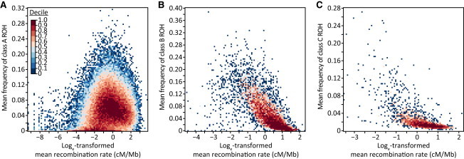
Relationship between ROH Frequency and Recombination Rate across the Genome

The figure shows heat maps for (A) class A (ρ = 0.171, p < 10⁻¹⁶), (B) class B (ρ = −0.785, p < 10⁻¹⁶), and (C) class C (ρ = −0.731, p < 10⁻¹⁶). Cells are colored by decile. The numbers of data points (nonoverlapping genomic windows) examined are 75,282, 7,013, and 2,994 for classes A, B, and C, respectively.

Table 3.

Spearman’s Correlation Coefficients between ROH Frequency and Recombination Rate

ROH Class	Number of Windows	ρ	p Value
A	75,254	0.171	<10−16
B	7,029	−0.785	<10−16
C	2,994	−0.731	<10−16

Signals of Recent Selection

Positive selection reduces haplotype diversity and increases homozygosity around the target locus, generating higher ROH frequencies in regions that harbor selection targets. This phenomenon is reflected in the observation that five of our top ten ROH hotspots overlapped regions previously identified as potential sites of recent positive selection.^33,57,59,60 Because selection acts over many generations, its effect might be expected to be greater on class A ROH and, to some extent, class B ROH than on class C ROH, which typically involve younger haplotypes produced by inbreeding. Conversely, as recent positive selection is expected to generate unusually long haplotypes,⁶⁸ we might expect that selection will have a greater influence on class C ROH than on the shorter ROH in classes A and B.

The relationship between iHS, a measure of positive selection based on haplotype patterns,⁴⁶ and ROH frequency produces several patterns (Figure 9). First, the frequencies of class A, B, and C ROH are generally positively correlated with iHS, supporting a role for natural selection in shaping genomic ROH patterns. Second, consistent with the latter hypothesis, the correlations between iHS and the frequency of class C ROH in each population exceed those between iHS and the frequencies of class A (p = 0.002, Wilcoxon signed-rank test) and B (p = 1.21 × 10⁻⁵) ROH, which were not significantly different (p = 0.515). These results are compatible with a scenario in which regions with homozygosity for the unusually long haplotypes created by recent selection events tend to be classified as class C ROH, whereas class A and B ROH created by older selection events either have weaker iHS signals or are partially diluted by the presence of class A and B ROH generated by other forces.

Figure 9.

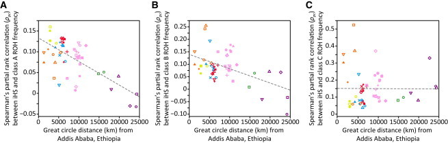
Relationship between iHS Selection Scores and ROH Frequencies in the 53 HGDP-CEPH Populations

The decrease of the Spearman’s partial rank correlation $\left({\rho }_{pc}\right)$ between iHS and ROH frequency with geographic distance from Addis Ababa is shown for (A) class A (R² = 0.468), (B) class B (R² = 0.253), and (C) class C (R² = 0.001) ROH. Populations are indicated by the same symbols as in Figure 4. Most ${\rho }_{pc}$ correlations had p < 0.05 (exceptions: A, Naxi and Surui; B, Papuan).

Third, the correlations between iHS and frequencies of class A and B ROH decrease with geographic distance from East Africa (R² = 0.468 and R² = 0.253, respectively), whereas the correlation with the frequency of class C ROH does not show such a pattern (R² = 0.001). This result is compatible with the observed increase in numbers of class A and B ROH with increasing distance from Africa (Figures S4A and S4B, respectively). These ROH result primarily from demographic processes rather than selection; demography drives class A and B ROH frequencies more strongly at a greater distance from Africa, and thus could progressively mask the influence of selection on ROH patterns. The lack of a negative correlation with class C ROH perhaps reflects a reduced impact of demography on class C ROH with increasing distance from Africa (Figure S4C).

OMIM versus Non-OMIM Genes

Genic regions represent the most conserved regions of the genome,⁶⁹ because amino-acid changes can alter protein function and lead to phenotypic changes. Consequently, functionally important variants, whether deleterious or beneficial, are expected to occur most often in or near genes. The influence of purifying selection on patterns of ROH might be most apparent at genes known to harbor deleterious alleles and whose disruption significantly influences fitness. For this reason, we compared genes implicated in Mendelian disorders with those that have not been so implicated.

Purifying selection is expected to increase levels of homozygosity; as strongly deleterious alleles might be expected to occur more frequently in OMIM genes than in non-OMIM genes, we expect ROH frequencies to be higher in OMIM genes than in non-OMIM genes. Additionally, as the correlations between iHS and the frequency of class C ROH significantly exceeded those with class A and B ROH frequencies, we might also expect a greater difference in the frequency of class C ROH between OMIM (separately for dominant and recessive diseases) and non-OMIM genes than in the frequencies of class A and B ROH.

Consistent with this expectation, whereas class C ROH were more frequent in genes associated with autosomal-dominant disease than in non-OMIM genes (p = 1.11 × 10⁻⁵, KS test; Table 4), class A and B ROH frequencies did not differ significantly between dominant and non-OMIM genes (p = 0.104 and p = 0.231, respectively). In comparison, class A, B, and C ROH frequencies were not significantly different between recessive and non-OMIM genes (p = 0.129, p = 0.106, and p = 0.089, respectively; Table 4). These results are compatible with deleterious alleles occurring more frequently in dominant-disease-associated genes than in non-OMIM genes. In addition, they are consistent with purifying selection removing deleterious dominant alleles, which are exposed to selection in both homozygotes and heterozygotes, more effectively than deleterious recessive alleles, which experience selection only in the rarer homozygous form.

Table 4.

Comparisons of ROH Frequencies between OMIM and Non-OMIM Genes

Variable 1	Variable 2	ROH Class	D	p Value
Autosomal-dominant genes (n = 515)	non-OMIM genes (n = 12,491)	A	−0.051	0.149
		B	0.048	0.207
		C	−0.063	0.039
Autosomal-recessive genes (n = 699)	non-OMIM genes (n = 12,491)	A	−0.045	0.129
		B	−0.047	0.106
		C	−0.048	0.089

p values are from two-sided Kolmogorov-Smirnov tests comparing runs-of-homozygosity (ROH) frequencies between two groups. Negative values of D indicate that group 1 (left) has higher frequencies than group 2 (right). Significant p values (<0.05) are highlighted in bold.

Discussion

Long ROH in humans are ubiquitous and frequent; they range in size from tens of kb to multiple Mb, and ROH of different sizes have different geographic distributions and patterns of occurrence across the genome. Per-individual total lengths of class A and class B ROH that reflect LD patterns are lowest in populations from Africa, rising in a stepwise fashion in successive continental groups and having relatively similar values within continents. This finding can be explained as a consequence of a serial-migration model outward from Africa; each migration decreases effective population size, generating LD, reducing haplotype diversity, and increasing the probability that identical copies of the same long haplotype will pair together in the same individual. The per-individual total lengths of class C ROH, which result largely from inbreeding, do not follow such a pattern and are instead most frequent in populations where isolation and consanguineous unions are more common. The different continental patterns observed for different ROH classes therefore reflect the distinct forces generating ROH of different sizes.

ROH hotspots potentially represent low-recombination regions, regions that may contain few deleterious recessive alleles and are thus able to maintain homozygosity, or locations of selective sweeps that have produced long tracts of extended haplotype homozygosity. By contrast, ROH coldspots might represent regions with high recombination rates, regions enriched for variants that have a severe negative impact on fitness in homozygotes, and thus cannot maintain homozygosity, or regions that harbor loci with heterozygous advantage and under selection favoring high haplotype diversity. We found that ROH hotspots were located throughout the genome, that their locations varied across continental regions, and that several of the most noticeable hotspots covered genomic regions that had previously been identified as sites of recent positive selection. These results suggest that positive selection is an important force driving the formation of ROH hotspots, and they raise the possibility that other hotspots we have identified might also result from positive selection. Consistent with this view, the positive correlation between selection signals and the frequencies of class A, B, and C ROH suggests that natural selection helps to shape patterns of genomic homozygosity over a broad range of evolutionary timescales.

We examined the possibility that the nonuniform genomic distribution of ROH might reflect correlations between ROH frequencies and other genomic variables and observed a negative correlation between recombination rate and class B and C ROH frequencies. This is in accordance with the view that by breaking long haplotypes, recombination will reduce the occurrence of long ROH. Curiously, however, we observed a weak positive correlation between recombination rate and the frequency of class A ROH, which suggests that the role of recombination in disrupting ROH is influenced by other factors that vary by ROH length and may reflect a faster transition from class B and C to class A ROH in high-recombination regions.

An additional possibility is that the heterogeneous distribution of copy-number-variable regions (CNVR) across the genome^70–72 might have influenced the genomic distribution of ROH we observed; certain types of copy-number changes can create long runs of erroneous homozygous genotype calls. If we compare CNVR previously identified in the 938 HGDP-CEPH individuals (HGDP Selection Browser; downloaded March 8^th, 2010) and 901 HapMap phase III individuals (downloaded January 27^th, 2011) to locations of ROH (Figure S8), we find that across individuals, on average only 0.12% of the total length of ROH overlaps CNVR (Figure S8D; SD = 0.19%, maximum = 1.7%). Thus, the genomic ROH distribution we report here is unlikely to have been strongly influenced by CNVR.

To investigate how deleterious dominant and recessive alleles might influence patterns of ROH frequencies, we separately compared mean ROH frequencies in genes known to be associated with autosomal-dominant or -recessive diseases to those in genes not associated with Mendelian disease. Mean class C ROH frequencies differed significantly between dominant and non-OMIM genes, but not between recessive and non-OMIM genes; this is compatible with the view that because purifying selection has a weaker effect on deleterious recessive loci than it does on deleterious dominant loci,⁷³ a difference in ROH frequency from non-OMIM loci is more likely for dominant than for recessive loci.

Several recent studies have produced related results on ROH patterns and the roles of different forces in producing ROH,^{4,6,20–22,24,25,31} and many studies have examined similar aspects of ROH to those we considered here.^{5,7,8,10,12,19,23,26–30} McQuillan et al.⁶ and Auton et al.,³¹ considering ROH primarily in Eurasians, remarked on the dual roles of ancient demographic history and consanguineous unions in producing ROH. Curtis et al.,²² Auton et al.,³¹ and Nothnagel et al.²⁵ further observed nonuniform distributions of genomic homozygosity, and recognized the existence of genomic regions where ROH were unusually frequent. Gibson et al.,²⁰ Li et al.,⁴ and Lencz et al.²¹ examined correlations of ROH with genomic variables, such as recombination rate and signals of positive selection. Notably, using an overlapping HGDP-CEPH data set, Kirin et al.²⁴ uncovered distinctive patterns of ROH in different populations, attributing them to the differing roles of demographic history and consanguineous unions in the various groups. However, they did not investigate the genomic distribution of ROH, its variability across populations, or its relationship to genomic variables. Finally, the studies of Leutenegger et al.⁵⁴ and Henn et al.,⁵⁵ which did not consider ROH, used HGDP-CEPH data to study variation across populations in related quantities, such as inbreeding coefficients and identity-by-descent tracts.

In addition to its contribution in combining many types of analysis of ROH into a comprehensive treatment of a large data set, our work provides a number of advances beyond past studies. First, most previous studies identified ROH using a genotype-counting approach that relies on a fixed number of homozygous sites within a sliding window of fixed size, allowing for occasional missing or heterozygous genotypes to account for possible genotyping errors. In contrast, our likelihood approach incorporates population-specific allele frequency estimates into the determination of the autozygosity status of a window, enabling more rigorous assessments of the possibility of genotyping errors and the loss of information caused by missing data. Indeed, a comparison of per-individual total lengths and numbers of ROH detected using likelihood-based and genotype-counting methods in our data set (Figure S9) and their overlap (Figure S10) suggests that the likelihood-based approach detects ROH more sensitively than does the genotype-counting approach. In addition, the likelihood-based approach provides a more precise measure of the probability that a given window is homozygous by chance; increasing the LOD-score threshold can enrich the ROH identified for those that probably represent autozygosity.

Second, previous studies classified ROH using a priori size boundaries applied to all populations, typically ignoring ROH shorter than ∼500 kb to exclude those ROH that may result from baseline LD patterns. This approach assumes that the distribution of ROH lengths is constant across populations, and therefore does not account for differences in this distribution that may derive from the distinct histories and consanguinity patterns of different populations. Our Gaussian-mixture approach instead accommodates population differences in the ROH length distribution by allowing boundaries between ROH size classes to vary across populations; furthermore, our mixture method does not ignore short ROH that result from baseline LD patterns, but instead treats them as a distinct class of ROH (class A). Despite their small size, these class A ROH derive from windows with high LOD scores and represent regions with genuine signals of autozygosity. The lower bound on ROH size in our analyses is determined primarily by the window length employed in the ROH-detection process; indeed, 96.7% of class A ROH we identified were smaller than 500 kb, as were 10.6% of all class B ROH. Additionally, whereas previous studies interpreted ROH of different sizes as resulting from different evolutionary mechanisms, our method builds an understanding of these mechanisms directly into ROH identification, placing ROH into different size classes that enable differences among populations to be more easily detected and interpreted. Finally, beyond these methodological advances, our inclusion of genomic comparisons with the frequency of each ROH class provides a more complete perspective on the determinants of ROH.

The patterns of ROH described here can provide a basis for improving specificity of disease-associated-gene identification in the context of homozygosity mapping. It has been hypothesized that thousands of genes associated with rare recessive disorders have yet to be discovered.⁷⁴ Such genes are often identified through homozygosity mapping in multigenerational consanguineous families. This approach sometimes yields too many candidate homozygous regions for efficient localization of the causal mutation.¹⁵ One approach to overcoming these problems is to increase the sample size by applying homozygosity mapping in outbred families^16,18 and individuals,^15,17 in whom homozygous regions are predicted to be smaller and less frequent. However, with the small sample sizes typical of rare diseases, the number of candidate regions can remain large. Our results on autosomal-recessive and non-OMIM genes suggest that the presence of a recessive-disease-associated gene in a genomic region is not predictive of its ROH frequency in a population sample of probably unaffected individuals; however, a region with high ROH frequency in affected individuals provides strong evidence for the presence of a disease-associated gene if it has a low frequency in unaffected individuals. Thus, many candidate regions might simply be regions in which ROH are common in the population, and those candidate regions with low population-level ROH frequencies are stronger candidates for further investigation. To facilitate the interpretation of homozygosity-mapping signals, we provide tables of genome-wide ROH frequencies for different ROH classes (Tables S2, S3, and S4), as well as of combined ROH frequencies over all three size classes (Table S5). This resource of baseline ROH frequencies in diverse human populations has the potential to accelerate the discovery of novel genes that underlie a wide variety of recessive disorders.

Supplemental Data

Table S2. The Frequency of Class A ROH at Each SNP in the Combined Data Set

ROH frequencies are given separately for each geographic region, as well as across all individuals in the data set.

Table S3. The Frequency of Class B ROH at Each SNP in the Combined Data Set

ROH frequencies are given separately for each geographic region, as well as across all individuals in the data set.

Table S4. The Frequency of Class C ROH at Each SNP in the Combined Data Set

ROH frequencies are given separately for each geographic region, as well as across all individuals in the data set.

Table S5. The Frequency of ROH Calculated over All Three Size Classes at Each SNP in the Combined Data Set

ROH frequencies are given separately for each geographic region, as well as across all individuals in the data set.

Web Resources

The URLs for data presented herein are as follows:

• Online Mendelian Inheritance in Man (OMIM), http://www.omim.org

• UCSC Human Genome Database, http://hgdownload.cse.ucsc.edu/downloads.html#human

• HapMap, http://hapmap.ncbi.nlm.nih.gov

• LocusZoom, http://csg.sph.umich.edu/locuszoom/

• HGDP Selection Browser, http://hgdp.uchicago.edu/

• pcor.test function for R, http://www.yilab.gatech.edu/pcor.html

References

- 1.Darwin C.R. John Murray; London, UK: 1876. The effects of cross and self fertilization in the vegetable kingdom. [Google Scholar]
- 2.Garrod A.E. The incidence of alkaptonuria: a study in chemical individuality. Lancet. 1902;160:1616–1620. [Google Scholar]
- 3.Mendel, G. (1866). Versuche über Pflanzenhybriden. Verhandlungen des naturforschenden Vereines in Brünn, 4, 3–47.
- 4.Li L.H., Ho S.F., Chen C.H., Wei C.Y., Wong W.C., Li L.Y., Hung S.I., Chung W.H., Pan W.H., Lee M.T. Long contiguous stretches of homozygosity in the human genome. Hum. Mutat. 2006;27:1115–1121. doi: 10.1002/humu.20399. [DOI] [PubMed] [Google Scholar]
- 5.Jakkula E., Rehnström K., Varilo T., Pietiläinen O.P., Paunio T., Pedersen N.L., deFaire U., Järvelin M.R., Saharinen J., Freimer N. The genome-wide patterns of variation expose significant substructure in a founder population. Am. J. Hum. Genet. 2008;83:787–794. doi: 10.1016/j.ajhg.2008.11.005. [DOI] [PMC free article] [PubMed] [Google Scholar]
- 6.McQuillan R., Leutenegger A.L., Abdel-Rahman R., Franklin C.S., Pericic M., Barac-Lauc L., Smolej-Narancic N., Janicijevic B., Polasek O., Tenesa A. Runs of homozygosity in European populations. Am. J. Hum. Genet. 2008;83:359–372. doi: 10.1016/j.ajhg.2008.08.007. [DOI] [PMC free article] [PubMed] [Google Scholar]
- 7.Gross A., Tönjes A., Kovacs P., Veeramah K.R., Ahnert P., Roshyara N.R., Gieger C., Rueckert I.M., Loeffler M., Stoneking M. Population-genetic comparison of the Sorbian isolate population in Germany with the German KORA population using genome-wide SNP arrays. BMC Genet. 2011;12:67. doi: 10.1186/1471-2156-12-67. [DOI] [PMC free article] [PubMed] [Google Scholar]
- 8.Humphreys K., Grankvist A., Leu M., Hall P., Liu J., Ripatti S., Rehnström K., Groop L., Klareskog L., Ding B. The genetic structure of the Swedish population. PLoS ONE. 2011;6:e22547. doi: 10.1371/journal.pone.0022547. [DOI] [PMC free article] [PubMed] [Google Scholar]
- 9.Woods C.G., Cox J., Springell K., Hampshire D.J., Mohamed M.D., McKibbin M., Stern R., Raymond F.L., Sandford R., Malik Sharif S. Quantification of homozygosity in consanguineous individuals with autosomal recessive disease. Am. J. Hum. Genet. 2006;78:889–896. doi: 10.1086/503875. [DOI] [PMC free article] [PubMed] [Google Scholar]
- 10.Hunter-Zinck H., Musharoff S., Salit J., Al-Ali K.A., Chouchane L., Gohar A., Matthews R., Butler M.W., Fuller J., Hackett N.R. Population genetic structure of the people of Qatar. Am. J. Hum. Genet. 2010;87:17–25. doi: 10.1016/j.ajhg.2010.05.018. [DOI] [PMC free article] [PubMed] [Google Scholar]
- 11.Lander E.S., Botstein D. Homozygosity mapping: a way to map human recessive traits with the DNA of inbred children. Science. 1987;236:1567–1570. doi: 10.1126/science.2884728. [DOI] [PubMed] [Google Scholar]
- 12.Broman K.W., Weber J.L. Long homozygous chromosomal segments in reference families from the centre d’Etude du polymorphisme humain. Am. J. Hum. Genet. 1999;65:1493–1500. doi: 10.1086/302661. [DOI] [PMC free article] [PubMed] [Google Scholar]
- 13.Botstein D., Risch N. Discovering genotypes underlying human phenotypes: past successes for Mendelian disease, future approaches for complex disease. Nat. Genet. 2003;33(Suppl):228–237. doi: 10.1038/ng1090. [DOI] [PubMed] [Google Scholar]
- 14.Gibbs J.R., Singleton A. Application of genome-wide single nucleotide polymorphism typing: simple association and beyond. PLoS Genet. 2006;2:e150. doi: 10.1371/journal.pgen.0020150. [DOI] [PMC free article] [PubMed] [Google Scholar]
- 15.Hildebrandt F., Heeringa S.F., Rüschendorf F., Attanasio M., Nürnberg G., Becker C., Seelow D., Huebner N., Chernin G., Vlangos C.N. A systematic approach to mapping recessive disease genes in individuals from outbred populations. PLoS Genet. 2009;5:e1000353. doi: 10.1371/journal.pgen.1000353. [DOI] [PMC free article] [PubMed] [Google Scholar]
- 16.Collin R.W., van den Born L.I., Klevering B.J., de Castro-Miró M., Littink K.W., Arimadyo K., Azam M., Yazar V., Zonneveld M.N., Paun C.C. High-resolution homozygosity mapping is a powerful tool to detect novel mutations causative of autosomal recessive RP in the Dutch population. Invest. Ophthalmol. Vis. Sci. 2011;52:2227–2239. doi: 10.1167/iovs.10-6185. [DOI] [PubMed] [Google Scholar]
- 17.Hagiwara K., Morino H., Shiihara J., Tanaka T., Miyazawa H., Suzuki T., Kohda M., Okazaki Y., Seyama K., Kawakami H. Homozygosity mapping on homozygosity haplotype analysis to detect recessive disease-causing genes from a small number of unrelated, outbred patients. PLoS ONE. 2011;6:e25059. doi: 10.1371/journal.pone.0025059. [DOI] [PMC free article] [PubMed] [Google Scholar]
- 18.Schuurs-Hoeijmakers J.H., Hehir-Kwa J.Y., Pfundt R., van Bon B.W., de Leeuw N., Kleefstra T., Willemsen M.A., van Kessel A.G., Brunner H.G., Veltman J.A. Homozygosity mapping in outbred families with mental retardation. Eur. J. Hum. Genet. 2011;19:597–601. doi: 10.1038/ejhg.2010.167. [DOI] [PMC free article] [PubMed] [Google Scholar]
- 19.Frazer K.A., Ballinger D.G., Cox D.R., Hinds D.A., Stuve L.L., Gibbs R.A., Belmont J.W., Boudreau A., Hardenbol P., Leal S.M., International HapMap Consortium A second generation human haplotype map of over 3.1 million SNPs. Nature. 2007;449:851–861. doi: 10.1038/nature06258. [DOI] [PMC free article] [PubMed] [Google Scholar]
- 20.Gibson J., Morton N.E., Collins A. Extended tracts of homozygosity in outbred human populations. Hum. Mol. Genet. 2006;15:789–795. doi: 10.1093/hmg/ddi493. [DOI] [PubMed] [Google Scholar]
- 21.Lencz T., Lambert C., DeRosse P., Burdick K.E., Morgan T.V., Kane J.M., Kucherlapati R., Malhotra A.K. Runs of homozygosity reveal highly penetrant recessive loci in schizophrenia. Proc. Natl. Acad. Sci. USA. 2007;104:19942–19947. doi: 10.1073/pnas.0710021104. [DOI] [PMC free article] [PubMed] [Google Scholar]
- 22.Curtis D., Vine A.E., Knight J. Study of regions of extended homozygosity provides a powerful method to explore haplotype structure of human populations. Ann. Hum. Genet. 2008;72:261–278. doi: 10.1111/j.1469-1809.2007.00411.x. [DOI] [PMC free article] [PubMed] [Google Scholar]
- 23.Nalls M.A., Simon-Sanchez J., Gibbs J.R., Paisan-Ruiz C., Bras J.T., Tanaka T., Matarin M., Scholz S., Weitz C., Harris T.B. Measures of autozygosity in decline: globalization, urbanization, and its implications for medical genetics. PLoS Genet. 2009;5:e1000415. doi: 10.1371/journal.pgen.1000415. [DOI] [PMC free article] [PubMed] [Google Scholar]
- 24.Kirin M., McQuillan R., Franklin C.S., Campbell H., McKeigue P.M., Wilson J.F. Genomic runs of homozygosity record population history and consanguinity. PLoS ONE. 2010;5:e13996. doi: 10.1371/journal.pone.0013996. [DOI] [PMC free article] [PubMed] [Google Scholar]
- 25.Nothnagel M., Lu T.T., Kayser M., Krawczak M. Genomic and geographic distribution of SNP-defined runs of homozygosity in Europeans. Hum. Mol. Genet. 2010;19:2927–2935. doi: 10.1093/hmg/ddq198. [DOI] [PubMed] [Google Scholar]
- 26.O’Dushlaine C.T., Morris D., Moskvina V., Kirov G., Consortium I.S., Gill M., Corvin A., Wilson J.F., Cavalleri G.L. Population structure and genome-wide patterns of variation in Ireland and Britain. Eur. J. Hum. Genet. 2010;18:1248–1254. doi: 10.1038/ejhg.2010.87. [DOI] [PMC free article] [PubMed] [Google Scholar]
- 27.Roy-Gagnon M.H., Moreau C., Bherer C., St-Onge P., Sinnett D., Laprise C., Vézina H., Labuda D. Genomic and genealogical investigation of the French Canadian founder population structure. Hum. Genet. 2011;129:521–531. doi: 10.1007/s00439-010-0945-x. [DOI] [PubMed] [Google Scholar]
- 28.Teo S.M., Ku C.S., Naidoo N., Hall P., Chia K.S., Salim A., Pawitan Y. A population-based study of copy number variants and regions of homozygosity in healthy Swedish individuals. J. Hum. Genet. 2011;56:524–533. doi: 10.1038/jhg.2011.52. [DOI] [PubMed] [Google Scholar]
- 29.Teo S.M., Ku C.S., Salim A., Naidoo N., Chia K.S., Pawitan Y. Regions of homozygosity in three Southeast Asian populations. J. Hum. Genet. 2012;57:101–108. doi: 10.1038/jhg.2011.132. [DOI] [PubMed] [Google Scholar]
- 30.Simon-Sanchez J., Scholz S., Fung H.C., Matarin M., Hernandez D., Gibbs J.R., Britton A., de Vrieze F.W., Peckham E., Gwinn-Hardy K. Genome-wide SNP assay reveals structural genomic variation, extended homozygosity and cell-line induced alterations in normal individuals. Hum. Mol. Genet. 2007;16:1–14. doi: 10.1093/hmg/ddl436. [DOI] [PubMed] [Google Scholar]
- 31.Auton A., Bryc K., Boyko A.R., Lohmueller K.E., Novembre J., Reynolds A., Indap A., Wright M.H., Degenhardt J.D., Gutenkunst R.N. Global distribution of genomic diversity underscores rich complex history of continental human populations. Genome Res. 2009;19:795–803. doi: 10.1101/gr.088898.108. [DOI] [PMC free article] [PubMed] [Google Scholar]
- 32.Li J.Z., Absher D.M., Tang H., Southwick A.M., Casto A.M., Ramachandran S., Cann H.M., Barsh G.S., Feldman M., Cavalli-Sforza L.L., Myers R.M. Worldwide human relationships inferred from genome-wide patterns of variation. Science. 2008;319:1100–1104. doi: 10.1126/science.1153717. [DOI] [PubMed] [Google Scholar]
- 33.Pickrell J.K., Coop G., Novembre J., Kudaravalli S., Li J.Z., Absher D., Srinivasan B.S., Barsh G.S., Myers R.M., Feldman M.W., Pritchard J.K. Signals of recent positive selection in a worldwide sample of human populations. Genome Res. 2009;19:826–837. doi: 10.1101/gr.087577.108. [DOI] [PMC free article] [PubMed] [Google Scholar]
- 34.International HapMap 3 Consortium. Altshuler D.M., Gibbs R.A., Peltonen L., Dermitzakis E., Schaffner S.F., Yu F., Bonnen P.E., de Bakker P.I., Deloukas P. Integrating common and rare genetic variation in diverse human populations. Nature. 2010;467:52–58. doi: 10.1038/nature09298. [DOI] [PMC free article] [PubMed] [Google Scholar]
- 35.Jakobsson M., Scholz S.W., Scheet P., Gibbs J.R., VanLiere J.M., Fung H.C., Szpiech Z.A., Degnan J.H., Wang K., Guerreiro R. Genotype, haplotype and copy-number variation in worldwide human populations. Nature. 2008;451:998–1003. doi: 10.1038/nature06742. [DOI] [PubMed] [Google Scholar]
- 36.Rosenberg N.A. Standardized subsets of the HGDP-CEPH Human Genome Diversity Cell Line Panel, accounting for atypical and duplicated samples and pairs of close relatives. Ann. Hum. Genet. 2006;70:841–847. doi: 10.1111/j.1469-1809.2006.00285.x. [DOI] [PubMed] [Google Scholar]
- 37.Weir B.S. Sinauer; Sunderland, MA: 1996. Genetic data analysis II. [Google Scholar]
- 38.Pemberton T.J., Wang C., Li J.Z., Rosenberg N.A. Inference of unexpected genetic relatedness among individuals in HapMap Phase III. Am. J. Hum. Genet. 2010;87:457–464. doi: 10.1016/j.ajhg.2010.08.014. [DOI] [PMC free article] [PubMed] [Google Scholar]
- 39.Rosenberg N.A., Mahajan S., Ramachandran S., Zhao C., Pritchard J.K., Feldman M.W. Clines, clusters, and the effect of study design on the inference of human population structure. PLoS Genet. 2005;1:e70. doi: 10.1371/journal.pgen.0010070. [DOI] [PMC free article] [PubMed] [Google Scholar]
- 40.Cann H.M., de Toma C., Cazes L., Legrand M.F., Morel V., Piouffre L., Bodmer J., Bodmer W.F., Bonne-Tamir B., Cambon-Thomsen A. A human genome diversity cell line panel. Science. 2002;296:261–262. doi: 10.1126/science.296.5566.261b. [DOI] [PubMed] [Google Scholar]
- 41.Rosenberg N.A., Mahajan S., Gonzalez-Quevedo C., Blum M.G., Nino-Rosales L., Ninis V., Das P., Hegde M., Molinari L., Zapata G. Low levels of genetic divergence across geographically and linguistically diverse populations from India. PLoS Genet. 2006;2:e215. doi: 10.1371/journal.pgen.0020215. [DOI] [PMC free article] [PubMed] [Google Scholar]
- 42.Wang S., Haynes C., Barany F., Ott J. Genome-wide autozygosity mapping in human populations. Genet. Epidemiol. 2009;33:172–180. doi: 10.1002/gepi.20344. [DOI] [PMC free article] [PubMed] [Google Scholar]
- 43.R Development Core Team (2011). R: A language and environment for statistical computing. R Foundation for Statistical Computing, Vienna. ISBN 3-900051-07-0, http://www.R-project.org.
- 44.Hintze J.L., Nelson R.D. Violin plots: A box plot-density trace synergism. Am. Stat. 1998;52:181–184. [Google Scholar]
- 45.Wang C., Szpiech Z.A., Degnan J.H., Jakobsson M., Pemberton T.J., Hardy J.A., Singleton A.B., Rosenberg N.A. Comparing spatial maps of human population-genetic variation using Procrustes analysis. Stat. Appl. Genet. Mol. Biol. 2010;9:13. doi: 10.2202/1544-6115.1493. [DOI] [PMC free article] [PubMed] [Google Scholar]
- 46.Voight B.F., Kudaravalli S., Wen X., Pritchard J.K. A map of recent positive selection in the human genome. PLoS Biol. 2006;4:e72. doi: 10.1371/journal.pbio.0040072. [DOI] [PMC free article] [PubMed] [Google Scholar]
- 47.Kim S.H., Yi S.V. Understanding relationship between sequence and functional evolution in yeast proteins. Genetica. 2007;131:151–156. doi: 10.1007/s10709-006-9125-2. [DOI] [PubMed] [Google Scholar]
- 48.Prugnolle F., Manica A., Balloux F. Geography predicts neutral genetic diversity of human populations. Curr. Biol. 2005;15:R159–R160. doi: 10.1016/j.cub.2005.02.038. [DOI] [PMC free article] [PubMed] [Google Scholar]
- 49.Ramachandran S., Deshpande O., Roseman C.C., Rosenberg N.A., Feldman M.W., Cavalli-Sforza L.L. Support from the relationship of genetic and geographic distance in human populations for a serial founder effect originating in Africa. Proc. Natl. Acad. Sci. USA. 2005;102:15942–15947. doi: 10.1073/pnas.0507611102. [DOI] [PMC free article] [PubMed] [Google Scholar]
- 50.Conrad D.F., Jakobsson M., Coop G., Wen X., Wall J.D., Rosenberg N.A., Pritchard J.K. A worldwide survey of haplotype variation and linkage disequilibrium in the human genome. Nat. Genet. 2006;38:1251–1260. doi: 10.1038/ng1911. [DOI] [PubMed] [Google Scholar]
- 51.Huang L., Jakobsson M., Pemberton T.J., Ibrahim M., Nyambo T., Omar S., Pritchard J.K., Tishkoff S.A., Rosenberg N.A. Haplotype variation and genotype imputation in African populations. Genet. Epidemiol. 2011;35:766–780. doi: 10.1002/gepi.20626. [DOI] [PMC free article] [PubMed] [Google Scholar]
- 52.Bittles A.H., Black M.L. Evolution in health and medicine Sackler colloquium: Consanguinity, human evolution, and complex diseases. Proc. Natl. Acad. Sci. USA. 2010;107(Suppl 1):1779–1786. doi: 10.1073/pnas.0906079106. [DOI] [PMC free article] [PubMed] [Google Scholar]
- 53.Bittles A.H., Black M.L. Consanguineous marriage and human evolution. Annu. Rev. Anthropol. 2010;39:193–207. [Google Scholar]
- 54.Leutenegger A.L., Sahbatou M., Gazal S., Cann H., Génin E. Consanguinity around the world: what do the genomic data of the HGDP-CEPH diversity panel tell us? Eur. J. Hum. Genet. 2011;19:583–587. doi: 10.1038/ejhg.2010.205. [DOI] [PMC free article] [PubMed] [Google Scholar]
- 55.Henn B.M., Hon L., Macpherson J.M., Eriksson N., Saxonov S., Pe’er I., Mountain J.L. Cryptic distant relatives are common in both isolated and cosmopolitan genetic samples. PLoS ONE. 2012;7:e34267. doi: 10.1371/journal.pone.0034267. [DOI] [PMC free article] [PubMed] [Google Scholar]
- 56.1000 Genomes Project Consortium A map of human genome variation from population-scale sequencing. Nature. 2010;467:1061–1073. doi: 10.1038/nature09534. [DOI] [PMC free article] [PubMed] [Google Scholar]
- 57.Sabeti P.C., Varilly P., Fry B., Lohmueller J., Hostetter E., Cotsapas C., Xie X., Byrne E.H., McCarroll S.A., Gaudet R., International HapMap Consortium Genome-wide detection and characterization of positive selection in human populations. Nature. 2007;449:913–918. doi: 10.1038/nature06250. [DOI] [PMC free article] [PubMed] [Google Scholar]
- 58.Tang K., Thornton K.R., Stoneking M. A new approach for using genome scans to detect recent positive selection in the human genome. PLoS Biol. 2007;5:e171. doi: 10.1371/journal.pbio.0050171. [DOI] [PMC free article] [PubMed] [Google Scholar]
- 59.Williamson S.H., Hubisz M.J., Clark A.G., Payseur B.A., Bustamante C.D., Nielsen R. Localizing recent adaptive evolution in the human genome. PLoS Genet. 2007;3:e90. doi: 10.1371/journal.pgen.0030090. [DOI] [PMC free article] [PubMed] [Google Scholar]
- 60.Coop G., Pickrell J.K., Novembre J., Kudaravalli S., Li J., Absher D., Myers R.M., Cavalli-Sforza L.L., Feldman M.W., Pritchard J.K. The role of geography in human adaptation. PLoS Genet. 2009;5:e1000500. doi: 10.1371/journal.pgen.1000500. [DOI] [PMC free article] [PubMed] [Google Scholar]
- 61.Lui V.C., Ng L.J., Sat E.W., Cheah K.S. The human alpha 2(XI) collagen gene (COL11A2): completion of coding information, identification of the promoter sequence, and precise localization within the major histocompatibility complex reveal overlap with the KE5 gene. Genomics. 1996;32:401–412. doi: 10.1006/geno.1996.0135. [DOI] [PubMed] [Google Scholar]
- 62.Richards A.J., Yates J.R., Williams R., Payne S.J., Pope F.M., Scott J.D., Snead M.P. A family with Stickler syndrome type 2 has a mutation in the COL11A1 gene resulting in the substitution of glycine 97 by valine in alpha 1 (XI) collagen. Hum. Mol. Genet. 1996;5:1339–1343. doi: 10.1093/hmg/5.9.1339. [DOI] [PubMed] [Google Scholar]
- 63.Griffith A.J., Sprunger L.K., Sirko-Osadsa D.A., Tiller G.E., Meisler M.H., Warman M.L. Marshall syndrome associated with a splicing defect at the COL11A1 locus. Am. J. Hum. Genet. 1998;62:816–823. doi: 10.1086/301789. [DOI] [PMC free article] [PubMed] [Google Scholar]
- 64.Miller C.T., Beleza S., Pollen A.A., Schluter D., Kittles R.A., Shriver M.D., Kingsley D.M. cis-Regulatory changes in Kit ligand expression and parallel evolution of pigmentation in sticklebacks and humans. Cell. 2007;131:1179–1189. doi: 10.1016/j.cell.2007.10.055. [DOI] [PMC free article] [PubMed] [Google Scholar]
- 65.Sulem P., Gudbjartsson D.F., Stacey S.N., Helgason A., Rafnar T., Magnusson K.P., Manolescu A., Karason A., Palsson A., Thorleifsson G. Genetic determinants of hair, eye and skin pigmentation in Europeans. Nat. Genet. 2007;39:1443–1452. doi: 10.1038/ng.2007.13. [DOI] [PubMed] [Google Scholar]
- 66.Bentwich I., Avniel A., Karov Y., Aharonov R., Gilad S., Barad O., Barzilai A., Einat P., Einav U., Meiri E. Identification of hundreds of conserved and nonconserved human microRNAs. Nat. Genet. 2005;37:766–770. doi: 10.1038/ng1590. [DOI] [PubMed] [Google Scholar]
- 67.Zhang R., Wang Y.Q., Su B. Molecular evolution of a primate-specific microRNA family. Mol. Biol. Evol. 2008;25:1493–1502. doi: 10.1093/molbev/msn094. [DOI] [PubMed] [Google Scholar]
- 68.Sabeti P.C., Schaffner S.F., Fry B., Lohmueller J., Varilly P., Shamovsky O., Palma A., Mikkelsen T.S., Altshuler D., Lander E.S. Positive natural selection in the human lineage. Science. 2006;312:1614–1620. doi: 10.1126/science.1124309. [DOI] [PubMed] [Google Scholar]
- 69.International Human Genome Sequencing Consortium Finishing the euchromatic sequence of the human genome. Nature. 2004;431:931–945. doi: 10.1038/nature03001. [DOI] [PubMed] [Google Scholar]
- 70.Redon R., Ishikawa S., Fitch K.R., Feuk L., Perry G.H., Andrews T.D., Fiegler H., Shapero M.H., Carson A.R., Chen W. Global variation in copy number in the human genome. Nature. 2006;444:444–454. doi: 10.1038/nature05329. [DOI] [PMC free article] [PubMed] [Google Scholar]
- 71.Kidd J.M., Cooper G.M., Donahue W.F., Hayden H.S., Sampas N., Graves T., Hansen N., Teague B., Alkan C., Antonacci F. Mapping and sequencing of structural variation from eight human genomes. Nature. 2008;453:56–64. doi: 10.1038/nature06862. [DOI] [PMC free article] [PubMed] [Google Scholar]
- 72.Conrad D.F., Pinto D., Redon R., Feuk L., Gokcumen O., Zhang Y., Aerts J., Andrews T.D., Barnes C., Campbell P., Wellcome Trust Case Control Consortium Origins and functional impact of copy number variation in the human genome. Nature. 2010;464:704–712. doi: 10.1038/nature08516. [DOI] [PMC free article] [PubMed] [Google Scholar]
- 73.Teshima K.M., Przeworski M. Directional positive selection on an allele of arbitrary dominance. Genetics. 2006;172:713–718. doi: 10.1534/genetics.105.044065. [DOI] [PMC free article] [PubMed] [Google Scholar]
- 74.Ropers H.H. New perspectives for the elucidation of genetic disorders. Am. J. Hum. Genet. 2007;81:199–207. doi: 10.1086/520679. [DOI] [PMC free article] [PubMed] [Google Scholar]
Associated Data
This section collects any data citations, data availability statements, or supplementary materials included in this article.
Supplementary Materials