Abstract
The objective of this study was to develop a probabilistic model to predict the end of lag time (λ) during the growth of Bacillus cereus vegetative cells as a function of temperature, pH, and salt concentration using logistic regression. The developed λ model was subsequently combined with a logistic differential equation to simulate bacterial numbers over time. To develop a novel model for λ, we determined whether bacterial growth had begun, i.e., whether λ had ended, at each time point during the growth kinetics. The growth of B. cereus was evaluated by optical density (OD) measurements in culture media for various pHs (5.5 ∼ 7.0) and salt concentrations (0.5 ∼ 2.0%) at static temperatures (10 ∼ 20°C). The probability of the end of λ was modeled using dichotomous judgments obtained at each OD measurement point concerning whether a significant increase had been observed. The probability of the end of λ was described as a function of time, temperature, pH, and salt concentration and showed a high goodness of fit. The λ model was validated with independent data sets of B. cereus growth in culture media and foods, indicating acceptable performance. Furthermore, the λ model, in combination with a logistic differential equation, enabled a simulation of the population of B. cereus in various foods over time at static and/or fluctuating temperatures with high accuracy. Thus, this newly developed modeling procedure enables the description of λ using observable environmental parameters without any conceptual assumptions and the simulation of bacterial numbers over time with the use of a logistic differential equation.
INTRODUCTION
Modeling of bacterial lag time is complicated because the mechanisms governing lag time are not fully understood. Early models of bacterial lag time described the log-transformed lag time using polynomial equations as functions of environmental factors (20). Later, the model proposed by Baranyi and Roberts (4) introduced the parameter α0, which represents the physiological state of bacterial cells. Their model focused on the constant relationship between h0 (= −ln α0), which refers to the “work to be done,” and the product of a specific growth rate (μmax) and the lag time (λ) (4, 36). Similarly, Mellefont et al. (21) introduced the concept of relative lag time, which represents the ratio of the lag time and the generation time. Although these models are mechanistic and appear robust, they do not consider the stochastic variability of the lag time. Stochastic variability in the behavior of single cells has recently received attention, and the variability of the lag time of single cells has been described as an appropriate probability distribution (12, 13, 19, 32, 33). However, although this modeling approach incorporates the probabilistic aspects of lag time, the deterministic aspects of lag time, such as the effects of environmental factors, have not been explicitly accounted for. Thus, although there have been numerous studies on bacterial lag time modeling, the modeling procedures developed to date have left room for improvement.
It is known that bacterial lag time is influenced not only by current environmental conditions but also by multiple other factors, such as the history of the cells and initial cell counts; however, the mechanisms of the lag time have not been completely clarified thus far. In previous lag time models, assumptions regarding h0 and the physiological state parameter (α0), which are directly unobservable conceptual variables, have been introduced to provide mechanistic and deterministic descriptions of the lag time. However, as the mechanisms of the lag time have not been completely clarified, we cannot avoid complications involved in developing a predictive lag time model based on various assumptions of directly unobservable conceptual parameters that consider various environmental factors and stochastic variabilities. Thus, under these circumstances, we focused on the development of a data-driven, empirical, and probabilistic model to describe the lag time based on experimentally observable data as a promising alternative.
The present study was aimed at developing a probabilistic lag time model that includes both the deterministic and probabilistic aspects of lag time. The probabilistic aspect of lag time can be described deterministically as a function of environmental factors. To provide baseline data for this study, we first determined whether bacterial growth had initiated; i.e., whether the lag time had ended at each time point was treated as the probability of that event occurring, which was modeled using logistic regressions as a function of time and other environmental parameters (1). The equation can be described as follows:
| (1) |
where P(t) is the probability of the end of lag time and f(t) is a function of time. The probability of the end of lag time can subsequently be described as a sigmoidal function with a value between 0 and 1.
We focused on the Baranyi and Roberts model (4) to apply the probabilistic lag time model described above. The Baranyi and Roberts model is one of the most frequently used differential equation models in predictive microbiology. It consists of the following two simultaneous differential equations:
| (2) |
| (3) |
where N denotes the bacterial cell concentration (CFU/g or CFU/ml) at time t, q is a dimensionless quantity related to the physiological state of the cells, μmax is the maximum specific growth rate (1/h), and Nmax represents the maximum population density of the bacteria (CFU/g or ml). Equation 2 can be explicitly solved as follows:
| (4) |
where q0 is the initial value of q at time zero. Then, equation 3 can be described by incorporating equation 4 as follows:
| (5) |
Equation 5 can be further modified as follows:
| (6) |
We focused on the function of
in equation 6, which adjusts the lag time as a value between 0 and 1, representing a sigmoidal change over time. However, because q is a dimensionless conceptual variable, it is difficult to use this variable to explicitly describe the effects of environmental and/or other factors. If an alternative function described by various factors could be substituted into equation 6 in place of
and still result in values between 0 and 1 with a sigmoidal increase over time, then bacterial growth simulation could be achieved successfully. The function of
is essentially the same as equation 1, which represents a logistic function. Thus, if the function of
could be replaced with a function of the probability of the end of lag time as described by the logistic regression given above, then the modified model of equation 6 could simulate bacterial densities over time.
The objective of the present study was to develop a statistical model for the probability of the end of bacterial lag time during growth kinetics using logistic regression as a function of time, temperature, pH, and sodium chloride concentration. The developed logistic regression model for lag time was subsequently combined with primary differential equations, such as the logistic model (Verhulst model) (28), to predict bacterial numbers over time. This new model was validated using experimentally obtained data on bacterial growth in real foods.
MATERIALS AND METHODS
Bacterial strain.
Bacillus cereus (BI-88, nonhemolytic enterotoxin producing, isolated from a crepe) was used as a target bacterium because it is a representative contaminant in cooked foods and demonstrates potential growth at low temperatures. The strain used in this study can grow at 8°C. The B. cereus culture was stored at −85°C in a medium containing 10% skim milk (Morinaga Milk Industry Co., Ltd., Tokyo, Japan). A sterile wire loop was used to transfer the frozen bacterial cultures to plate count agar (Eiken Ltd., Tokyo, Japan). The plate was incubated at 35°C for 18 h. A typical single colony was inoculated in a glass tube containing 10 ml of tryptic soy broth (TSB; Difco Ltd., Franklin Lakes, NJ) and incubated at 35°C for 18 h without agitation. Subsequently, 1 ml of the culture was inoculated in 10 ml of fresh TSB and incubated at 35°C for 6 h without agitation. The growth medium consisting of the vegetative cells was used as an inoculum.
B. cereus growth experiments.
Peptone-yeast extract-glucose (PYG) broth containing yeast extract (2.0 g/liter; Difco), peptone (5.0 g/liter, Difco), and glucose (1.0 g/liter; Wako, Ltd., Tokyo, Japan) was used as a base medium for the B. cereus growth experiments (18, 24). Hydrochloric acid (HCl; Wako) was used to adjust the pH of the medium to 5.5, 6.0, 6.5, and 7.0. Sodium chloride (NaCl; Wako) was also added to the PYG medium at concentrations of 0.5, 1.0, 1.5, and 2.0% (wt/vol). These media were filtered through a membrane filter (pore size, 0.45 μm; Millipore Ltd., Billerica, MA), and a 5-ml aliquot was transferred to an L-shaped glass tube. The inoculum consisting of vegetative cells of B. cereus (0.1 ml) was added to 5 ml of broth (ca. 105 CFU/ml) and incubated at 10, 15, and 20°C.
To validate the model, independent conditions from the model development were examined within the interpolation region of the model. The growth data were obtained at 12 and 17°C for pH values of 5.8, 6.3, and 6.7 and NaCl concentrations of 0.7, 1.2, and 1.7%.
Optical density measurement of B. cereus growth and determination of the lag time.
B. cereus growth was monitored by optical density (OD) measurements at 660 nm using a Bio-photorecorder (model TVS062CA; Advantec Toyo Roshi Kaisha, Ltd., Tokyo, Japan). This apparatus can continuously and automatically measure and record the OD values in an L-shaped glass tube at various temperatures. The OD values were recorded every 10 min until they reached 1.0. B. cereus growth curves for each condition given above were obtained in triplicate.
In the present study, the lag time of B. cereus was defined as the time required for the OD to increase by 0.006 from the beginning of the incubation (0.000). The value of 0.006 was chosen because it represents the smallest detectable significant change in OD values for the given sensitivity of the apparatus (0.001) and the measurement noise (0.003 to 0.005).
In parallel, the lag time was estimated by the previously reported procedure using OD data and viable counts (8). Briefly, the nontransformed four-parameter logistic model fit the OD growth curves as follows (9):
| (7) |
where t is time, ODmax and ODmin are asymptotic maximum and minimum OD values, respectively, μOD is μmax determined from OD values, and ti is the time at the inflection point in equation 7. Then, the time (tΔOD) and viable counts (NΔOD) corresponding to a 0.05-unit increase in OD values were determined from fitted model parameter values. The lag time was then calculated by using equation 8:
| (8) |
where values of N0 and NΔOD were determined from viable counts, and other parameters are as described above.
Modeling the probability of the end of lag time.
As described above, the end of the lag time of B. cereus was defined as the detection of a change of >0.006 OD unit at 660 nm during the incubation period. Each replicate sample was assigned a value of 1 or 0 to indicate whether or not the end of the B. cereus lag time had been reached, respectively. The data were fitted to a logistic regression model using R statistical software (v 2.14.1; www.R-project.org/) based on a previously developed approach (16) in which we used the “glm” function. The two models proposed in this study were of the following form:
| (9) |
| (10) |
where, Logit(P) represents ln[P/(1 − P)], ln is the natural logarithm, P is the probability of growth initiation (or the end of the lag time), which has a value between 0 and 1, ai and bi are the coefficients to be estimated, Temp is the temperature (°C), Time is the time of incubation (h), pH is the pH of the tested environment, and NaCl is the concentration (%) of sodium chloride in the tested environment. We used the logarithm of the incubation time because this factor would have a nonlinear effect on the end of the lag time.
Simulation of the population size of B. cereus.
We applied the developed probability model for the end of the lag time, as described above, to equation 6 as a substitute for
. Equations 9 and 10 can be transformed into the following equations:
| (11) |
| (12) |
Therefore, the following model equations were proposed:
| (13) |
| (14) |
The model for determining the μmax value of B. cereus was obtained from ComBase Predictor (http://modelling.combase.cc/ComBase_Predictor.aspx). The μmax model for B. cereus employed by ComBase Predictor is as follows (kindly provided by J. Baranyi):
| (15) |
where Temp and pH are as described above and bw corresponds to
. aw was calculated using the following equation (29):
| (16) |
Nmax was set at 108 CFU/g. Equations 13 and 14 were solved numerically using the fourth-order Runge-Kutta method to obtain predictions of the bacterial concentrations using the “odesolve” package in the R statistical software.
Evaluation of model performance.
The performance of the developed lag time model was evaluated using the following procedures. The area under the receiver-operating characteristic curve (AUC) (14), maximum rescaled R2, and percent concordance were used as measures of the goodness of fit of the developed model. In addition, the performance of the lag time model was evaluated using the acceptable prediction zone method (26). The prediction errors or relative errors (REs) for the individual fitted cases were calculated according to the following equation:
| (17) |
An RE of less than 0 represents fail-safe predictions, and an RE greater than 0 represents fail-dangerous predictions. The proportion of RE (pRE) in the acceptable prediction zone of −0.6 to 0.3 was used to quantify the performance of the lag time model. The performance of the lag time model was classified as acceptable for a pRE value of ≥0.70 (26). The performance of the combined models (equations 13 and 14) for the bacterial number over time was evaluated using the root mean squared error (RMSE) (20).
B. cereus growth in foods under static conditions.
Six types of Japanese deli food (cooked pumpkin, cooked okara [soy pulp, a residue of tofu production], cooked burdock roots and carrots, cooked satoimo [a taro], cooked freeze-dried tofu, and lightly salted cooked freeze-dried tofu) were used for the model validation. All sample foods were either obtained from a local manufacturer (pumpkins, okara, burdock, and carrot) or cooked in the laboratory (satoimo and freeze-dried tofu). The pH and NaCl concentration of the sample foods were determined using a pH meter (D-51; Horiba, Kyoto, Japan) and a compact salt meter (C-121; Horiba), respectively. Samples of 25 ± 1 g of each deli food were aseptically divided into plastic pouches (deposition as follows: 12 μm polyethylene terephthalate [PET], 15 μm oriented nylon [ONY], and 6 µm cast polypropylene [CPP], with a thickness of 33 μm) at each sampling interval. An aliquot of 0.1 ml of the B. cereus (3 to 4 log CFU/g) vegetative cell suspension, which was prepared as described above, was inoculated onto each deli food. The inoculated foods were aerobically stored at 10 or 15°C for up to 7 days (168 h). Sampling was generally conducted at 12- and 6-h intervals for the samples at 10 and 15°C, respectively. Each experiment consisted of two independent replicates and two plates per replicate at each time interval.
B. cereus growth in food under fluctuating-temperature conditions.
The model performance was validated under fluctuating-temperature conditions. B. cereus vegetative cells were inoculated into two cream pasta sauces (pH 6.20 and 1.05% NaCl; pH 5.95 and 1.59% NaCl) in the same manner as the other deli foods mentioned above. The inoculated pasta sauces were aerobically stored under fluctuating temperature conditions that consisted of 10°C storage with some temperature fluctuations over an 80-h storage period. The temperature data were recorded using a temperature logger (Thermo recorder TR-71S; T&D Corporation, Nagano, Japan) and were used for the simulation of B. cereus growth using the developed models (equations 13 and 14).
Enumeration of B. cereus.
Each food sample (25 ± 1 g) was combined with 225 ml of 0.1% peptone water in a 400-ml stomacher bag and was processed for 1 min in a stomacher (Organo Ltd., Tokyo, Japan). The sample suspension was then serially diluted in 0.1% peptone-water. The diluted sample was plated in duplicate (0.1 ml) on Kim and Goepfert (KG) agar with NaCl and glycine (NGKG) (15) (Nissui Pharmaceutical Ltd., Tokyo, Japan), which is a selective medium for B. cereus, and incubated at 35°C for 24 h.
RESULTS
Comparison of the lag times (λ) estimated by two methods.
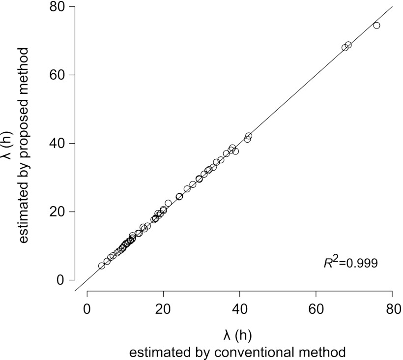
The λs estimated by the changes in OD values (>0.006) were very closely correlated to the λs estimated from the curve-fitting (equations 7 and 8) procedure (Fig. 1). Because the λs estimated by curve fitting procedure to OD values were consistent with those estimated by viable counts (8), the small but significant OD changes employed in the present study appropriately estimated the lag time of bacterial growth.
Fig 1.
Relationship of the estimated lag times between the conventional curve fitting procedure (8) and the method employed in the present study.
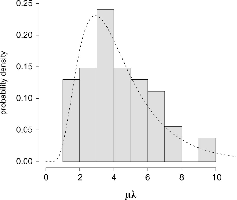
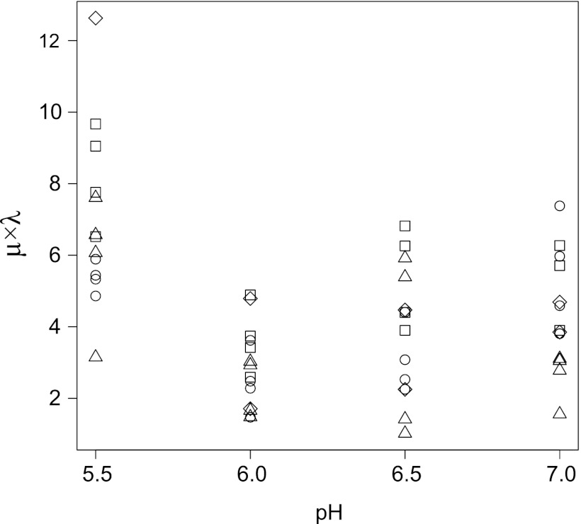
The parameters such as μmax and λ were obtained through the curve-fitting procedure of the OD growth data. The products of μmax and λ were not constant but were distributed as shown in Fig. 2. The distribution of values of μmax × λ was fitted with a log-normal distribution. Furthermore, there was no NaCl concentration and/or pH dependency on the μmax × λ (Fig. 3). Since an apparent inverse proportionality between μmax and λ was not confirmed, a separate modeling of the λ from μmax was investigated in the present study.
Fig 2.
Distribution of the product of estimated specific growth rate (μmax) and lag time (λ). The dotted line is a fitted probability distribution as a function of log-normal (mean = 1.34, standard deviation = 0.52).
Fig 3.
pH and/or NaCl dependency of the μmaxλ. □, 0.5% NaCl; ○, 1.0% NaCl; △, 1.5% NaCl; □, 2.0% NaCl.
Modeling the probability of the end of lag time.
The growth initiation response of B. cereus to various environmental conditions was monitored, resulting in a total of 45,222 data points collected during the incubation period. The 45,222 data points were analyzed using the developed logistic regression models described in equations 9 and 10. The estimated parameters and their 95% confidence intervals are given in Table 1 along with the performance statistics of the AUC, maximum rescaled R2, and percent concordance. Figure 4a shows an example of the cumulative probability distribution estimated from the developed models derived from equations 11 and 12. Figure 4b shows the corresponding probability density distribution that is calculated by the differentiation of equations 11 and 12. The performance statistics indicate a good performance of both models, with little difference between them (Table 1 and Fig. 4). Although Akaike's information criterion (AIC) for equation 9 was slightly larger than that for equation 10 (Table 1), we chose the simpler model, equation 9, for further study because with the simpler model, the effects of each environmental factor are easier to calculate and interpret.
Table 1.
Estimated parameters of logistic regression models
| Equation and parameter | Estimate (mean) | 95th percentile |
SE | |
|---|---|---|---|---|
| 2.5% | 97.5% | |||
| Equation 9a | ||||
| Intercept | −21.449 | −22.025 | −20.879 | 0.292 |
| ln (time) | 3.105 | 3.043 | 0.574 | 0.032 |
| temp | 0.560 | 0.546 | 3.169 | 0.007 |
| pH | 0.960 | 0.899 | 1.022 | 0.031 |
| Salt | −0.955 | −1.017 | −0.894 | 0.031 |
| Equation 10b | ||||
| Intercept | −14.619 | −16.257 | −12.984 | 0.834 |
| ln(time) | 3.322 | 3.254 | 3.392 | 0.035 |
| Temp | −0.364 | −0.476 | −0.253 | 0.056 |
| pH | −0.877 | −1.134 | −0.620 | 0.131 |
| Salt | 4.526 | 3.782 | 5.273 | 0.380 |
| Temp × pH | 0.200 | 0.182 | 0.219 | 0.009 |
| Temp × salt | −0.202 | −0.221 | −0.184 | 0.009 |
| pH × salt | −0.488 | −0.598 | −0.379 | 0.055 |
AUC of equation 9, 0.95; max rescaled R2, 0.70; concordance, 95.8%; AIC, 22,971.
AUC of equation 10, 0.95; max rescaled R2, 0.71; concordance, 96.1%; AIC, 22,055.
Fig 4.
Representative changes in the probability of the end of lag time at pH 6.0 and 0.5% NaCl. (a) The cumulative probability distribution predicted by equation 11 (solid lines) and equation 12 (dashed lines). (b) Probability density distributions calculated by differentiation of equation 11 (solid lines) and equation 12 (dashed lines).
Validation with independent OD growth data in the interpolation region.
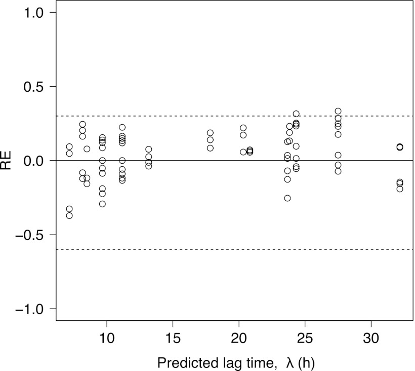
The developed model for the probability of end of lag time in equation 9 was validated using independent data sets derived from the conditions of the interpolation region of the developed model. The λs predicted by the developed model were calculated at a P value of 0.5. For these independent data, 52 of 54 (3 pH conditions × 3 NaCl conditions × 2 temperature conditions in triplicate) REs (%RE = 97.7%) were within the acceptable prediction zone (−0.6 to 0.3) (Fig. 5). No prediction problems or regional biases were encountered. Thus, the model for the probability of end of lag time had an acceptable goodness of fit and was validated for interpolation.
Fig 5.
Relative error (RE) plots comparing the observed and predicted values (at P = 0.5) of the lag time of B. cereus fitted by equation 9. The dotted lines represent the acceptable prediction zone for an RE of −0.6 (fail-safe) to 0.3 (fail-dangerous).
Validation using bacterial growth data in cooked foods under static conditions.
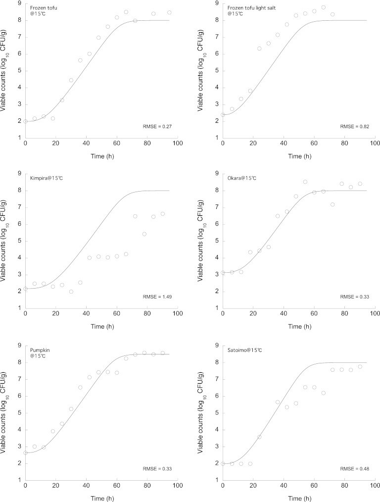
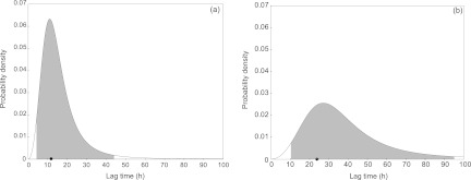
The experimentally observed changes in the number of B. cereus cells on various Japanese deli foods and the growth simulation given by equation 13 incorporated into the ComBase Predictor μmax model using the pH and NaCl concentration of each food (Table 2) are shown in Fig. 6 and 7. The overall predictions during storage, regardless of the storage temperature or the type of food, were consistent with the observed B. cereus number, with relatively small RMSEs (Fig. 6 and 7). The λs were estimated from the observed growth data using the DMFit software (4) (Table 2). The accuracy of the model prediction was good under all food and temperature conditions (Table 2). All of the observed λs fell within the 95% prediction interval of the predicted probability distribution. Compared with other predictions of λs of B. cereus vegetative cells based on polynomial models, such as the Pathogen Modeling Program (PMP) (6), the ComBase Predictor, and the model devised by Ölmez and Aran (25), the observed results and those predicted by the model developed in the present study indicated relatively shorter λs. While the pRE (≥0.70) was in the acceptable prediction zone of the λ (−0.6 to 0.3), demonstrating acceptable performance of the developed lag time model, the other models were not acceptable (pRE < 0.70). The probability distributions of the end of the lag time derived using the differentiation of equation 11 for the growth of bacteria in cooked okara (soy pulp, tofu residue) are shown in Fig. 8 as a representative result. The observed λs fell within the 95% prediction intervals of the newly developed model. Thus, this newly developed model for the lag time enabled a description of the probability distribution of the lag time and could also be combined with a bacterial growth differential equation model to accurately simulate bacterial growth.
Table 2.
Comparison of the observed and predicted lag times of B. cereus inoculated on cooked foods
| Food | pH | NaCl (%) | Temp (°C) | Lag time (h) |
||||
|---|---|---|---|---|---|---|---|---|
| Observeda | Predictedb [95% PIc] | CBPd | PMPe | Reference 25f | ||||
| Freeze-dried tofu | 6.92 | 1.7 | 15 | 16.5 | 13.2 [4.0–42.3] | 24.5 | 23.0 | 22.3 |
| 10 | 28.3 | 32.6 [10.0–105.9] | 52.4 | 103.7 | 70.3 | |||
| Freeze-dried tofu, lightly salted | 7.09 | 0.40 | 15 | 6.1 | 8.4 [2.6–27.3] | 22.1 | 14.4 | 9.8 |
| 10 | 7.2 | 20.8 [6.4–67.4] | 53.2 | 61.2 | 37.7 | |||
| Satoimo (taro) | 5.49 | 0.49 | 15 | 8.2 | 14.2 [4.3–46.0] | 32.6 | 18.1 | 20.5 |
| 10 | 22.9 | 35.0 [10.8–113.6] | 63.0 | 69.6 | 77.6 | |||
| Pumpkin | 6.18 | 0.57 | 15 | 7.8 | 11.8 [3.6–38.1] | 27.6 | 12.2 | 13.6 |
| 10 | 35.7 | 28.9 [8.9–94.1] | 62.3 | 49.4 | 51.0 | |||
| Okara (soy pulp) | 6.37 | 1.25 | 15 | 15.4 | 13.7 [4.2–44.3] | 27.4 | 15.6 | 20.1 |
| 10 | 30.8 | 33.7 [10.3–109.4] | 61.3 | 66.7 | 67.8 | |||
| Burdock root and carrot | 5.72 | 1.45 | 15 | 29.6 | 17.8 [5.4–57.7] | 34.2 | 20.0 | 32.1 |
| 10 | 53.2 | 43.7 [13.4–142.3] | 73.2 | 83.2 | 104.9 | |||
| pREg | 0.75 | 0.25 | 0.33 | 0.33 | ||||
Estimated by fitting growth curve using DMFit.
Predicted value at P = 0.5.
PI, prediction interval.
Prediction by the ComBase predictor (physiological state value was set as default: 0.000611).
Prediction by the Pathogen Modeling Program.
Prediction by the model of Ölmez and Aran.
Proportion of relative error (pRE) in the acceptable prediction zone of lag time (−0.3 to 0.6).
Fig 6.
Experimentally observed changes in the number of B. cereus cells on Japanese deli foods and the growth prediction calculated using equation 13 at 10°C.
Fig 7.
Experimentally observed changes in the number of B. cereus cells on Japanese deli foods and the growth prediction calculated using equation 13 at 15°C.
Fig 8.
Probability density distributions of the end of lag time for cooked okara at 15°C (a) and 10°C (b) derived using the differentiation of equation 11. The shaded area represents the 95% prediction interval, and the filled circle represents the observed lag time estimated by using DMFit software.
Validation using bacterial growth data under fluctuating temperatures.
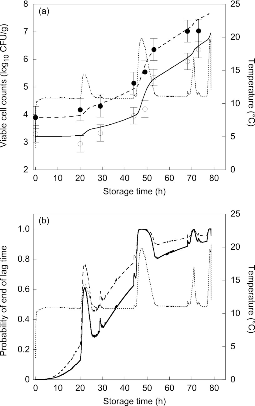
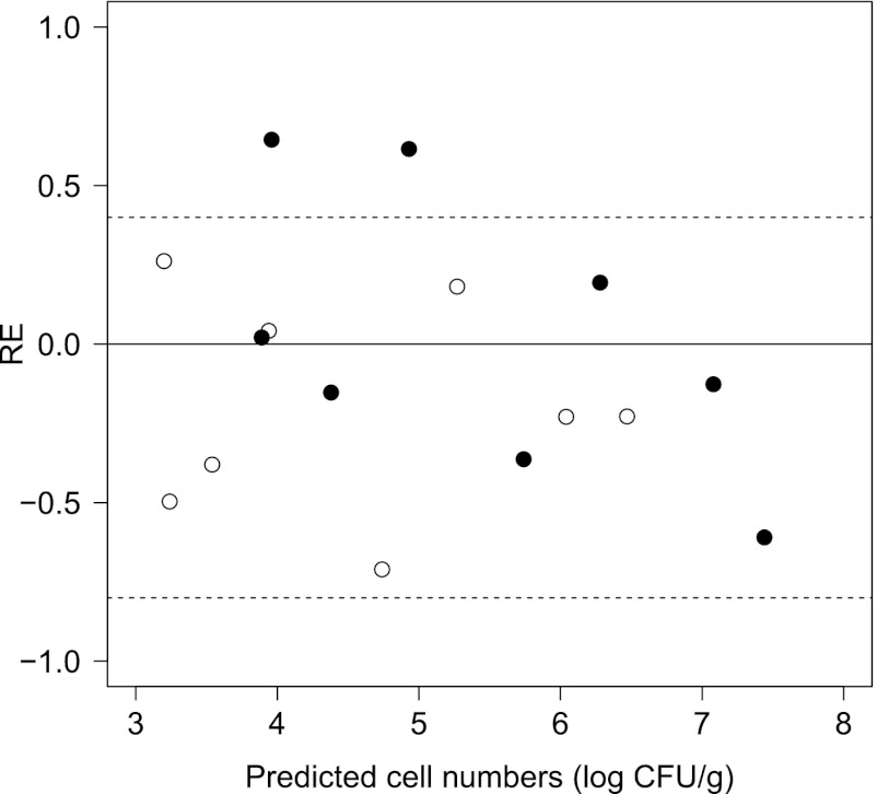
The experimentally observed changes in the number of B. cereus cells in cream pasta sauces under fluctuating temperature conditions and the growth simulation given by equation 12 incorporated into the ComBase Predictor μmax model using the values of pH and NaCl concentration of each pasta sauce are shown in Fig. 9a. The overall model predictions during storage, regardless of the conditions (pH or salt concentration) of the sauce, were consistent with the observed B. cereus number, with RMSEs of less than 0.2 log CFU/g. Although the probability of the end of lag time basically increased with time, the changes in the probability of the end of lag time followed the temperature shifts (Fig. 9b). The changes in the probability of the end of lag time seemed to adjust to the increase in B. cereus during the storage period. The pRE of B. cereus cell numbers within the acceptable prediction zone (−0.8 to 0.4) (26) was 87.5%, representing an acceptable performance (Fig. 10). Moreover, no prediction problems or regional biases were encountered (Fig. 10). Thus, the developed model illustrated acceptable accuracy under fluctuating temperatures.
Fig 9.
(a) Experimentally observed changes in the number of B. cereus cells in cream pasta sauces and the growth prediction under fluctuating temperatures calculated using equation 13. The dotted line represents changes in temperature. Filled and open circles represent the observed B. cereus number (log CFU/g) in sauces I (pH 6.20, 1.05% NaCl) and II (pH 5.95, 1.59% NaCl), respectively. The dashed and solid lines represent model predictions for sauces I and II, respectively. The root mean squared errors for sauces I and II were 0.17 and 0.18, respectively. (b) Probability of the end of lag time corresponding to temperature changes. The dotted line represents changes in temperature. The dashed and solid lines represent model predictions for sauces I and II, respectively.
Fig 10.
Relative error (RE) plots comparing the observed and predicted values of the number of B. cereus cells calculated by equation 13 under fluctuating temperature conditions. The dotted lines represent the acceptable prediction zone for an RE of −0.8 (fail-safe) to 0.4 (fail-dangerous). Filled and open circles represent the results for sauces I (pH 6.20, 1.05% NaCl) and II (pH 5.95, 1.59% NaCl), respectively.
DISCUSSION
The function adjusting the lag time plays a key role in describing the bacterial numbers over time using a differential equation model such as the Baranyi and Roberts model (4). The function
, which adjusts the lag time in the Baranyi and Roberts model, shows a sigmoidal increase over time with values between 0 and 1. With the adjusting function, the differential equation model can exhibit lag duration in a growth curve. However, although the adjusting function in the Baranyi and Roberts model is based on the assumption α0 that is based on constancy of μmax × λ, the values of μmax × λ are not always constant, as shown in the present study (Fig. 2) as well as the other literature (2, 10, 21, 31). The distribution of the values for μmax × λ presented here is similar to those in previous studies. Since this conceptual relationship should therefore be applied with caution, there is room for improvement in the adjusting function of lag time combined with a differential equation. Because lag time is apparently highly variable for various reasons, it might be difficult to describe the lag time as a deterministic function. To take into account the various factors influencing lag time duration, a probabilistic approach would be better to describe the complexity of lag time. Thus, an alternative modeling of lag time describing it as a probability function without any biological and/or conceptual assumption was investigated in the present study.
The model developed in the present study for the probability of the end of the lag time is not based on any biological and/or conceptual assumption. Because a logistic regression model was simply fitted to the experimental data, the flexibility of the model is improved over that of other procedures that rely on prior assumptions. A mechanistic approach to modeling that is based on biological and/or conceptual assumptions is critical to future improvement; however, until the mechanism governing bacterial lag time is understood, the benefit of modeling the lag time based on biological and/or conceptual assumptions is unclear. Thus, empirical modeling driven by experimental data remains an important procedure.
The developed logistic regression model for the probability of the end of lag time demonstrated high goodness of fit as representing a high AUC value (0.95) and high concordance (95.8%). In contrast, the maximum rescaled R2 value was not very high (0.70). However, because it has been reported that the R2 does not accurately reflect the goodness of fit of the logistic regression model, as it does that of the linear regression model (1), this result was not surprising. From the validation results shown in Fig. 3 and Table 2, it has been illustrated that the developed model enabled accurate prediction of the lag time. The lag time could be successfully described as a probability function of time and environmental factors that can be directly measured.
The OD growth kinetics data were used in the present study to develop the model for the probability of the end of lag time during the growth kinetics. In order to determine accurate timing of the end of lag time, OD measurement with short measuring intervals (10 min) was employed. However, the most important point is not the measurement of OD value itself but an appropriate determination of the lag time ending. Although the defined small but significant OD change in the present study successfully reflected the lag time ending (Fig. 1), the OD change would not reflect real end of lag time in the case of a smaller inoculum. Because the changes in OD value are below the detection limit at lower inoculum levels, such as <104 CFU/ml, the changes in OD value would be biased toward zero and could not detect the end of lag time appropriately. In such cases, the end of lag time can be estimated by other procedures, such as time-to-detection measurement with a 2-fold dilution method (5, 7), plate counts, and other high-resolution enumeration methods. The end of lag time determined by those methods would also be applied to the probabilistic model development as described in the introduction. This feature would allow us to increase the choices for more accurate and flexible model development.
Many authors have observed that abrupt changes in environmental conditions, such as temperature, pH, and aw, during the growth phase induce an “intermediate” lag phase (17, 21–23, 34, 37). It has been reported that abrupt environmental changes cause cells to perform extra work before reinitiating their growth. Some authors have proposed models for the effects of temperature shifts on the lag time of Escherichia coli (34), Lactobacillus plantarum (36), and Listeria monocytogenes (35). Delignette-Muller et al. (11) highlighted a linear relationship between the work to be done and the magnitude and direction of temperature shifts. Although the intermediate lag times caused by abrupt changes in environmental conditions are commonly neglected in tertiary models that simulate bacterial numbers over time, Muñoz-Cuevas et al. (23) recently proposed a procedure for incorporating intermediate lag times induced by temperature shifts. Moreover, Le Marc et al. (17) proposed a procedure for incorporating intermediate lag times induced by pH and/or osmotic shifts. Muñoz-Cuevas et al. (23) successfully described the intermediate lag time by reflecting the changes in h(t) (remaining work to be done) as a square root function of temperature and aw. These procedures are based on the theoretical parameter h0, which is derived from the assumption of a constant product of μmax and λ. This approach is totally mechanistic, and the relationship between μmax and λ is indispensable.
In contrast, the procedure developed in the present study is a completely data-driven empirical approach without any conceptual and/or biological assumptions. The procedure allows us to determine lag time independent of h0 and μmax. This approach allowed us to develop a flexible model. As mentioned above, the model developed in the present study successfully simulated bacterial numbers over time with temperature fluctuations (Fig. 6a). Moreover, the results of the changes in the probability of the lag time ending (Fig. 6b) may reflect the intermediate lag time corresponding to temperature shifts. While the approach of the present study is not mechanistic, as is the approach by Muñoz-Cuevas et al. (23), this simple data-driven empirical modeling procedure using logistic regression offers the possibility of considering the intermediate lag time as a change in the probability of the end of lag time. Further studies are required to investigate the ability to estimate the intermediate lag time between the developed empirical method and other mechanistic approaches.
The bacterial lag time is affected by the current environmental conditions, as well as various other factors, such as the history of the population or cell, preculturing conditions, the magnitude and rate of change in the environment (11, 21, 22, 35), initial cell counts (3, 27, 30), and strain variability. In the present study, we did not employ these factors as parameters; however, we could use the effects of the population history, initial cell counts, and strain variability as parameters in a logistic regression model due to the flexible nature of the model. Because logistic regressions employ various types of data as explanatory variables (1), we could develop a model for the probability of the end of lag time that would consider the effects mentioned above if sufficient data sets became available. The availability of data sets is a critical and challenging problem for the modeling procedure developed in the present study and should be addressed in future studies.
Using single-cell behavior as an approach to accounting for variability among bacterial cells has recently received attention, and the variability of single-cell lag times has been modeled as a probability distribution (12, 13, 19, 32, 33). This modeling approach has drawn attention to risk assessors, because the nature of such models emphasizes the variability of the lag time. The model developed in the present study enabled us to illustrate the probability distribution of the lag time by differentiation of the model equation, as shown in Fig. 4b and 8. However, the distribution derived from the developed model reflects the distribution of the population lag time. If single-cell lag time data were applied to a logistic regression, such as that developed in the present study, the lag distribution of single-cell variability could be described. This possibility will be considered for future studies involving the model developed here.
In conclusion, the newly developed model for the probability of end of lag time will allow us to develop more flexible models without additional biological assumptions. Although some problems to be examined remain, this modeling procedure represents an effective alternative for predicting bacterial lag time.
Footnotes
Published ahead of print 22 June 2012
REFERENCES
- 1. Agresti A. 2007. An introduction to categorical data analysis, 2nd ed. John Wiley & Sons, Inc., Hoboken, NJ [Google Scholar]
- 2. Augustin J-C, Carlier V. 2000. Mathematical modelling of the growth rate and lag time for Listeria monocytogenes. Int. J. Food Microbiol. 56: 29–51 [DOI] [PubMed] [Google Scholar]
- 3. Baranyi J, Pin C. 1999. Estimating bacterial growth parameters by means of detection times. Appl. Environ. Microbiol. 65: 732–736 [DOI] [PMC free article] [PubMed] [Google Scholar]
- 4. Baranyi J, Roberts T. 1994. A dynamic approach to predicting bacterial-growth in food. Int. J. Food Microbiol. 23: 277–294 [DOI] [PubMed] [Google Scholar]
- 5. Biesta-Peters EG, Reij MW, Joosten H, Gorris LGM, Zwietering MH. 2010. Comparison of two optical-density-based methods and a plate count method for estimation of growth parameters of Bacillus cereus. Appl. Environ. Microbiol. 76: 1399–1405 [DOI] [PMC free article] [PubMed] [Google Scholar]
- 6. Buchanan RL. 1993. Developing and distributing user-friendly application software. J. Ind. Microbiol. 12: 251–255 [Google Scholar]
- 7. Cuppers HGAM, Smelt JPPM. 1993. Time to turbidity measurement as a tool for modeling spoilage by Lactobacillus. J. Ind. Microbiol. Biotechnol. 12: 168–171 [Google Scholar]
- 8. Dalgaard P, Koutsoumanis K. 2001. Comparison of maximum specific growth rates and lag times estimated from absorbance and viable count data by different mathematical models. J. Microbiol. Methods 43: 183–196 [DOI] [PubMed] [Google Scholar]
- 9. Dalgaard P, Ross T, Kamperman L, Neumeyer K, McMeekin TA. 1994. Estimation of bacterial growth rates from turbidimetric and viable count data. Int. J. Food Microbiol. 23: 391–404 [DOI] [PubMed] [Google Scholar]
- 10. Delignette-Muller M. 1998. Relation between the generation time and the lag time of bacterial growth kinetics. Int. J. Food Microbiol. 43: 97–104 [DOI] [PubMed] [Google Scholar]
- 11. Delignette-Muller ML, Baty F, Cornu M, Bergis H. 2005. Modelling the effect of a temperature shift on the lag phase duration of Listeria monocytogenes. Int. J. Food Microbiol. 100: 77–84 [DOI] [PubMed] [Google Scholar]
- 12. Francois K, et al. 2005. Modelling the individual cell lag phase: effect of temperature and pH on the individual cell lag distribution of Listeria monocytogenes. Int. J. Food Microbiol. 100: 41–53 [DOI] [PubMed] [Google Scholar]
- 13. Guillier L, Augustin J-C. 2006. Modelling the individual cell lag time distributions of Listeria monocytogenes as a function of the physiological state and the growth conditions. Int. J. Food Microbiol. 111: 241–251 [DOI] [PubMed] [Google Scholar]
- 14. Hosmer DW, Lemeshow S. 2000. Applied logistic regression, 2nd ed. Wiley & Sons, New York, NY [Google Scholar]
- 15. Kim HU, Goepfert JM. 1971. Enumeration and identification of Bacillus cereus in foods. I. 24-hour presumptive test medium. Appl. Microbiol. 22: 581–587 [DOI] [PMC free article] [PubMed] [Google Scholar]
- 16. Koseki S, Matsubara M, Yamamoto K. 2009. Prediction of a required log reduction with probability for Enterobacter sakazakii during high-pressure processing, using a survival/death interface model. Appl. Environ. Microbiol. 75: 1885–1891 [DOI] [PMC free article] [PubMed] [Google Scholar]
- 17. Le Marc Y, Skandamis P, Belessi C. 2010. Modeling the effect of abrupt acid and osmotic shifts within the growth region and across growth boundaries on adaptation and growth of Listeria monocytogenes. Appl. Environ. Microbiol. 76: 6555–6563 [DOI] [PMC free article] [PubMed] [Google Scholar]
- 18. McCann K, et al. 2005. Isolation and characterisation of antibacterial peptides derived from the f (164–207) region of bovine α S2-casein. Int. Dairy J. 15: 133–143 [Google Scholar]
- 19. McKellar RC, Hawke A. 2006. Assessment of distributions for fitting lag times of individual cells in bacterial populations. Int. J. Food Microbiol. 106: 169–175 [DOI] [PubMed] [Google Scholar]
- 20. McKellar RC, Lu X. 2004. Modeling microbial responses in food. CRC Press, Boca Raton, FL [Google Scholar]
- 21. Mellefont L, McMeekin T, Ross T. 2003. The effect of abrupt osmotic shifts on the lag phase duration of foodborne bacteria. Int. J. Food Microbiol. 83: 281–293 [DOI] [PubMed] [Google Scholar]
- 22. Mellefont LA, Ross T. 2003. The effect of abrupt shifts in temperature on the lag phase duration of Escherichia coli and Klebsiella oxytoca. Int. J. Food Microbiol. 83: 295–305 [DOI] [PubMed] [Google Scholar]
- 23. Muñoz-Cuevas M, Fernández PS, George S, Pin C. 2010. Modeling the lag period and exponential growth of Listeria monocytogenes under conditions of fluctuating temperature and water activity values. Appl. Environ. Microbiol. 76: 2908–2915 [DOI] [PMC free article] [PubMed] [Google Scholar]
- 24. Murdock CA, Matthews KR. 2002. Antibacterial activity of pepsin-digested lactoferrin on foodborne pathogens in buffered broth systems and ultra-high temperature milk with EDTA. J. Appl. Microbiol. 93: 850–856 [DOI] [PubMed] [Google Scholar]
- 25. Ölmez HK, Aran N. 2005. Modeling the growth kinetics of Bacillus cereus as a function of temperature, pH, sodium lactate and sodium chloride concentrations. Int. J. Food Microbiol. 98: 135–143 [DOI] [PubMed] [Google Scholar]
- 26. Oscar TP. 2005. Development and validation of primary, secondary, and tertiary models for growth of Salmonella Typhimurium on sterile chicken. J. Food Prot. 68: 2606–2613 [DOI] [PubMed] [Google Scholar]
- 27. Pascual C, Robinson TP, Ocio MJ, Aboaba OO, Mackey BM. 2001. The effect of inoculum size and sublethal injury on the ability of Listeria monocytogenes to initiate growth under suboptimal conditions. Lett. Appl. Microbiol. 33: 357–361 [DOI] [PubMed] [Google Scholar]
- 28. Peleg M, Corradini MG, Normand MD. 2007. The logistic (Verhulst) model for sigmoid microbial growth curves revisited. Food Res. Int. 40: 808–818 [Google Scholar]
- 29. Resnik SL, Chirife J. 1988. Proposed theoretical water activity values at various temperatures for selected solutions to be used as reference sources in the range of microbial growth. J. Food Prot. 51: 419–423 [DOI] [PubMed] [Google Scholar]
- 30. Robinson T, et al. 2001. The effect of inoculum size on the lag phase of Listeria monocytogenes. Int. J. Food Microbiol. 70: 163–173 [DOI] [PubMed] [Google Scholar]
- 31. Ross T. 1999. Predictive microbiology models in the meat industry. Meat and Livestock Australia, Sydney, Australia [Google Scholar]
- 32. Standaert AR, et al. 2007. Modeling individual cell lag time distributions for Listeria monocytogenes. Risk Anal. 27: 241–254 [DOI] [PubMed] [Google Scholar]
- 33. Stringer SC, Webb MD, Peck MW. 2011. Lag time variability in individual spores of Clostridium botulinum. Food Microbiol. 28: 228–235 [DOI] [PubMed] [Google Scholar]
- 34. Swinnen IAM, Bernaerts K, Gysemans K, Van Impe JF. 2005. Quantifying microbial lag phenomena due to a sudden rise in temperature: a systematic macroscopic study. Int. J. Food Microbiol. 100: 85–96 [DOI] [PubMed] [Google Scholar]
- 35. Whiting RC, Bagi LK. 2002. Modeling the lag phase of Listeria monocytogenes. Int. J. Food Microbiol. 73: 291–295 [DOI] [PubMed] [Google Scholar]
- 36. Zwietering MH, Cuppers HG, de Wit JC, van't Riet K. 1994. Evaluation of data transformations and validation of a model for the effect of temperature on bacterial growth. Appl. Environ. Microbiol. 60: 195–203 [DOI] [PMC free article] [PubMed] [Google Scholar]
- 37. Zwietering MH, de Wit JC, Cuppers HG, van't Riet K. 1994. Modeling of bacterial growth with shifts in temperature. Appl. Environ. Microbiol. 60: 204–213 [DOI] [PMC free article] [PubMed] [Google Scholar]


