Abstract
Purpose: Micro-CT is widely used for small animal imaging in preclinical studies of cardiopulmonary disease, but further development is needed to improve spatial resolution, temporal resolution, and material contrast. We present a technique for visualizing the changing distribution of iodine in the cardiac cycle with dual source micro-CT.
Methods: The approach entails a retrospectively gated dual energy scan with optimized filters and voltages, and a series of computational operations to reconstruct the data. Projection interpolation and five-dimensional bilateral filtration (three spatial dimensions + time + energy) are used to reduce noise and artifacts associated with retrospective gating. We reconstruct separate volumes corresponding to different cardiac phases and apply a linear transformation to decompose these volumes into components representing concentrations of water and iodine. Since the resulting material images are still compromised by noise, we improve their quality in an iterative process that minimizes the discrepancy between the original acquired projections and the projections predicted by the reconstructed volumes. The values in the voxels of each of the reconstructed volumes represent the coefficients of linear combinations of basis functions over time and energy. We have implemented the reconstruction algorithm on a graphics processing unit (GPU) with CUDA. We tested the utility of the technique in simulations and applied the technique in an in vivo scan of a C57BL/6 mouse injected with blood pool contrast agent at a dose of 0.01 ml/g body weight. Postreconstruction, at each cardiac phase in the iodine images, we segmented the left ventricle and computed its volume. Using the maximum and minimum volumes in the left ventricle, we calculated the stroke volume, the ejection fraction, and the cardiac output.
Results: Our proposed method produces five-dimensional volumetric images that distinguish different materials at different points in time, and can be used to segment regions containing iodinated blood and compute measures of cardiac function.
Conclusions: We believe this combined spectral and temporal imaging technique will be useful for future studies of cardiopulmonary disease in small animals.
Keywords: dual energy, micro-CT, spectral, cardiac, small animal imaging
INTRODUCTION
Micro-CT is widely used for small animal imaging in preclinical studies of cardiopulmonary disease.1 However, the small size of the mouse heart (5 mm diameter) and the rapid heart rate (up to 600 beats per minute [bpm]) present substantial technical challenges.
Functional cardiac imaging requires the monitoring of the ECG signal during the micro-CT scan. The monitoring can be performed extrinsically, with electrodes or a pulse oximeter, or intrinsically, by observing the motion of the heart in the projection images.2, 3 This signal can be used to time the acquisition of x-ray projections to coincide with distinct phases of the heart (prospective gating), or the projections can be acquired at a constant rate and the signal can be used after the scan to allocate the projections to different phases (retrospective gating). Prospective gating ensures equiangular distribution of projections, but it involves longer scan times and greater technical complexity.4 Retrospective gating is faster and simpler to implement, but it generates projections with an irregular angular distribution, which can result in reconstructed volumes afflicted by streaking artifacts.5 In both strategies, once the projections are acquired, images of the heart at several phases of the cardiac cycle can be reconstructed separately. However, many of the features in these images are preserved over time, and there has been growing interest in exploiting this redundancy in the reconstruction process to improve image quality and reduce scan time and radiation dose.6 Some promising strategies include iterative reconstruction algorithms that use temporal information as a starting condition or a constraint.7 Other strategies extend noise reduction techniques such as bilateral filtration to the temporal domain.8
Iodinated contrast agents are typically used to distinguish the blood from the surrounding tissue. However, conventional CT produces a single value at each voxel, the attenuation coefficient, which complicates efforts to quantify the concentration of iodine when other materials are present in varying concentrations. In order to better distinguish the contrast agent, dual energy imaging is commonly used. In this technique, scans are acquired with two different spectral settings. These differences can be obtained by changing the x-ray tube voltage9 or adding filters,10 and can be implemented with one x-ray tube changing over time,11 two x-ray tubes and detectors,12 or overlaid detectors.13 Once the projections are acquired at these different settings and reconstructed separately, the contrast agent and the surrounding tissue can be decomposed in postprocessing.14 However, this approach tends to amplify the noise in the reconstructed images and is especially sensitive to geometric errors. As with temporal reconstruction, efforts have been made to exploit the substantial overlap of information between the two scans within the reconstruction process.15, 16, 17
In this work, we present a technique to visualize the changing distribution of iodine in the body with a dual source micro-CT system, using a retrospectively gated dual energy scan with optimized filters and voltages, and a series of computational operations to reconstruct the data. This results in five-dimensional volumetric images that distinguish different materials at different points in time and can be used to segment regions containing iodinated blood and compute various measures of cardiac function, such as the stroke volume, the ejection fraction, and the cardiac output. We test the utility of the separate steps in simulations, and then demonstrate the technique in an in vivo scan of a mouse.
THEORY
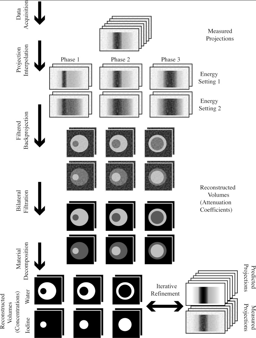
Our method uses retrospective gating to acquire temporal information, and dual energy material decomposition to acquire spectral information. Both of these techniques are imperfect, and their problems compound: Retrospective gating tends to produce reconstructed images that are afflicted by streaking artifacts and noise, and dual energy material decomposition tends to amplify these undesirable properties. To reduce the artifacts and noise, we employ projection interpolation (Sec. 2A) and bilateral filtration (Sec. 2B). To reduce the amplification of the artifacts and noise, we optimize the spectral properties of our data acquisition protocol (Sec. 2C), and we iteratively refine the results of the material decomposition (Sec. 2D). Some of these steps present computational challenges that must be overcome (Sec. 2E), and some depend upon a physically accurate spectral model of our system (Sec. 2F). The utility of these various steps are demonstrated in simulations (Sec. 3A). The entire method is summarized in Fig. 1. Unless otherwise noted, all calculations were performed in MATLAB (The MathWorks, Natick, MA).
Figure 1.
A diagram of the proposed technique.
Projection interpolation
During the scan, while the projections are acquired, the animal's cardiac and respiratory signals are recorded. After acquisition, the phases in the cardiac and respiratory signals are identified by thresholding the signals along with their first and second derivatives. These three thresholds are found in an iterative procedure that minimizes the standard deviation of the duration of the cycles. At each iteration, a new set of three thresholds are chosen, the thresholds are used to label the peaks, the times between the peaks are found, and the standard deviation of the set of times between the peaks is calculated. When this standard deviation converges, the procedure stops, and the final set of three thresholds are used to identify the peaks. Each projection is then assigned a relative time between 0 and 1 for each signal (cardiac or respiratory) identifying the fraction of the cycle elapsed since the most recent peak.
The projections can then be allocated to sets based on their phases in the cardiac and respiratory cycles, and these sets can be reconstructed separately with conventional reconstruction algorithms, such as filtered backprojection (FBP).18 However, because the projection acquisition and the physiological processes of the animal are in general uncorrelated, the angular distribution of the projections in each set will be irregular, and this results in streaking artifacts in the images reconstructed with FBP.5 To overcome this problem, we generate synthetic sets of projections with a regular angular distribution by interpolating the projections in each set, using the following method.
The projections acquired at a given tube setting are distinguished by their angle, their cardiac phase, and their respiratory phase. An interpolated projection Pi at a particular angle αi and phase ϕi is a weighted average of all the acquired projections Pj, with the weights determined by a function w of the distances between the interpolated angle and phase and the acquired angles and phases:
| (1) |
where
P is a projection, a two-dimensional array of values measured on the detector.
i is the index of the interpolated projection.
j is the index of the acquired projection.
α is the angle of the projection.
αs is the step angle between the interpolated projections.
ϕ is the phase of the projection (cardiac or respiratory).
nϕ is the number of phases to be reconstructed.
Here, w is a Gaussian weight function used for both angle and phase values:
| (2) |
where
a is an angle or phase.
d is the maximum allowable distance between ai and aj.
n is the maximum possible value of a.
[ai, aj]n is a distance function on a cyclical domain from 0 to n:
| (3) |
The value of the step angle αs between the interpolated projections is chosen according to the desired tradeoff between the image quality at each phase and the temporal blurring between phases. In general, this value is scan-dependent. The same formulas apply to both respiratory and cardiac imaging. In the case of the cardiac imaging performed in this study, in addition to the cardiac phases, we weight the projections by their distance from the end-expiration phase of the respiratory cycle in order to reduce motion blur caused by respiratory motion.
Bilateral filtration
Because of the limited numbers of photons and projections available at each phase, and some residual streaking artifacts left by the projection interpolation, the reconstructed images are still noisy. To denoise the images we use bilateral filtration.19 This technique is similar to smoothing by convolution with a Gaussian kernel. In conventional Gaussian smoothing, the value at a voxel μ(r) at position r is replaced by a weighted average of its neighbors μ′(r), and the contribution of each neighboring voxel is determined by the distance between the neighbor and the voxel being modified:
| (4) |
where
| (5) |
and σ is the standard deviation of the Gaussian.
In bilateral filtration, however, the contribution is also weighted by the difference in the values of the neighboring voxel and the modified voxel:
| (6) |
where σd and σr are referred to as the domain and range parameters, respectively. In other words, this technique favors the contributions of voxels that look similar and suppresses the contributions of voxels that look different. This has the effect of preserving edges while reducing noise.
To extend this technique beyond three dimensions, we include the time inside the domain, and make μ a function with two values at each point, corresponding to each tube setting:
| (7) |
where [t, t′]1 is the cyclical distance that we described in Sec. 2A, and ‖‖2 is the L2 norm. The filtration is applied to all the volumes from each time and energy setting, combined together into a five-dimensional data structure. This approach is similar to the five-dimensional bilateral filtration employed by Sawall et al.8
To use this technique, appropriate values must be found for σd, σt, and σr. We set these parameters based on heuristic criteria, and their values are scan-dependent. σd is set so that the spatial neighborhood is no larger than 5 × 5 voxels, since larger neighborhoods are computationally demanding. σt is set so that no temporal neighborhood extends beyond one time point before or after, to minimize temporal blurring. σr is set to be less than the difference in intensities between bone and soft tissue at the low energy setting, and less than the difference in intensities between iodine and soft tissue at the high energy setting, to minimize the contributions of voxels from different materials.
Material decomposition
The projections are acquired at two different energy settings simultaneously, and images at each setting and at each cardiac phase are reconstructed separately. After performing bilateral filtration on these images, we apply a linear transformation to separate the images into components corresponding to water and iodine. We represent the attenuation coefficients at each energy setting at each point in time and space as a linear combination of the attenuation coefficients of water and iodine:
| (8) |
where cwater and ciodine are the concentrations of water and iodine, respectively. The values of the material coefficients μwater, low, μiodine, low, μwater, high, and μiodine, high are measured in manually selected regions in vials containing known concentrations of these materials that are attached to the animal cradle. The concentrations of water and iodine in the rest of the image are then found through matrix inversion:
| (9) |
We apply this transformation from attenuation space to material space separately to each cardiac phase. This material decomposition is standard in the field.14
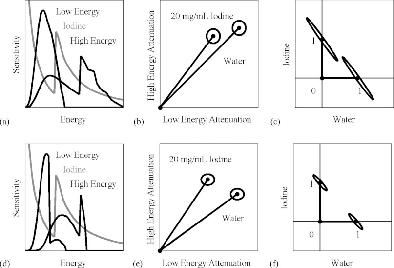
Unfortunately, this decomposition has the effect of amplifying noise. The reason can be seen in Fig. 2, which shows the spectral sensitivity functions at the different energy settings of our system compared to the attenuation spectrum of iodine (a) and (d); the expected attenuation values of water and iodine at these energy settings (b) and (e); and the decomposed fractional concentrations of water and iodine (c) and (f). The rows of the matrix to be inverted in Eq. 9 correspond to the vectors in attenuation space (b) and (e), which are almost collinear. Regions of uncertainty, defined by the standard deviations of the measurements of the materials, are represented as ellipses. The closer the vectors are to each other, the more the domain is stretched out when the transformation is performed, and the regions of uncertainty in material space are severely elongated. Our choice of energy settings is directed toward maximizing the angle between these vectors in order to minimize the elongation of the regions of uncertainty.
Figure 2.
The material decomposition can be represented as a linear transformation from attenuation space (b) and (e) to material space (c) and (f). The attenuation coefficients for water and iodine are represented by vectors, and the axes of the ellipses around the vectors are the standard deviations of these measurements in a typical scan with our micro-CT system (b), (e). These correspond to the vectors and ellipses representing the relative concentrations (0–1) of water and iodine (c) and (f). When the energy settings are suboptimal (a), the vectors corresponding to water and iodine are close together (b), and the transformation amplifies the noise (c). When a better set of energy settings are chosen (d), the water and iodine vectors are farther apart (e), and the noise amplification is less pronounced (f). The condition number of the decomposition matrix corresponding to the improved settings is less than half of the condition number for the original settings.
This elongation is predicted by the condition number.20 The condition number of a function is a measure of how small changes in the inputs might be amplified by the function. The higher the condition number, the greater the possible amplification, and the lower the accuracy in the presence of noise. For matrices, such as in Eq. 9, the condition number is equal to the ratio of the maximum and minimum singular values.
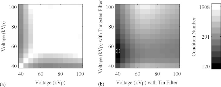
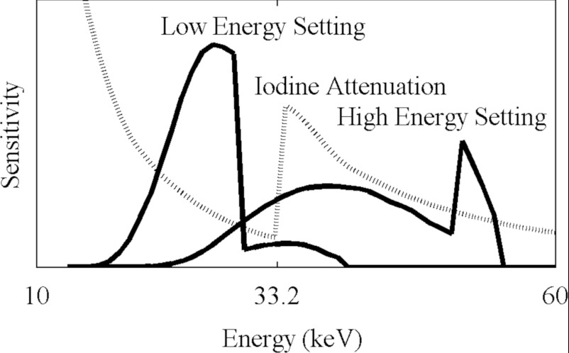
We used this metric to determine the optimal energy settings. We first searched for a pair of filters to shape the spectrum. We surveyed the periodic table and compiled a list of metals that are available in sheets or plates that are solid, stable, and nontoxic; with sufficient thickness to absorb between one-third and two-thirds of the incident radiation; and that have absorption spectra that predominantly block photons either above or below the K-edge of iodine, 33.2 keV. We found that tin is effective at suppressing energies above this value, and tungsten below this value. We then considered various combinations of voltages on the x-ray tubes. At each pair of voltages between 40 kVp and 100 kVp, we calculated the average attenuation coefficients of water and iodine, with and without the filters, and calculated the condition number of the matrix in Eq. 9. These numbers are displayed in Fig. 3. We selected the combination of voltages and filters that produce the lowest condition number. The resulting spectral sensitivity functions for our system are shown in Fig. 4.
Figure 3.
The condition number of the material decomposition matrix as a function of voltage, without (a) and with (b) filters. The darkest region in B, 40 kVp with the tin filter and 55 kVp with the tungsten filter, indicated with the crosshairs, corresponds to the lowest condition number.
Figure 4.
The spectral sensitivity of our system with the two x-ray energy settings. These functions include the contributions from the tube, filters, and detector.
Iterative refinement
The resulting material images are still compromised by noise. To improve the quality of the images, we apply a refinement that iteratively reduces the discrepancy between the original acquired projections and the projections predicted by the reconstructed volumes. In the previous steps, the acquired projections were allocated to different sets based on their spectral and temporal properties and reconstructed separately. However, this strategy ignored the considerable overlap in the spectra of the different tube settings and the different materials in the object, as well as the overlap of the normalized exposure times of the projections. In the refinement, the values in the voxels of each of the reconstructed volumes represent the coefficients of linear combinations of basis functions over time and energy, and we use all the acquired projections to refine the estimates of these coefficients. The contribution of each projection to the volume representing the coefficient for a particular basis function is proportional to the degree of overlap between the basis function and the temporal and spectral sensitivity of the system when the projection was acquired.
This algorithm is based on several prior techniques.15, 16, 17 However, our method is unique in its combination of both time and energy information in the same formula.
We construct a formula to represent the spectral x-ray image acquisition process at the N pixel measurements from the x-ray detector in terms of the M voxels of the object being imaged. The expected photon count at pixel measurement i is:
| (10) |
where
is the spectral sensitivity function, i.e., the number of x-ray photons at energy e scaled by the detector response at e. This function is described in greater detail in Sec. 2F. The values of this function for our system are shown in Fig. 4.
μj(e) is the attenuation coefficient of voxel j at energy e.
aij is the length of the portion of the x-ray trajectory from the x-ray source to pixel i that intersects voxel j.
Here, and aij are determined by experimental design and calibration procedures, while μj(e) is to be reconstructed.
The actual photon count pi is a random variable, which is often modeled as a sample from a Poisson distribution:
| (11) |
This distribution is only an approximation, for it ignores the polychromatic nature of the radiation, as well as the noise introduced by the indirect conversion at the scintillator and the electronic noise on the detector. The decision to represent the photon count as a deterministic value with additive noise or as a value selected at random from a known distribution influences the choice of the reconstruction algorithm, described below.
The goal of the spectral reconstruction process is to recover μ(e) at all voxels from p at all pixel measurements. μj(e) is represented as a linear combination of D basis functions:
| (12) |
where each basis function fd(e) is chosen in advance based on the known spectral properties of the object, and the coefficient cjd of basis function d at voxel j is unknown. Possible sets of basis functions include the relative contributions to attenuation of Compton scatter and the photoelectric effect,9 or energy bins,15 but in this study we have chosen the mass attenuation curves of water and iodine, since the goal of this spectral reconstruction process is to find the concentration of iodine at all voxels, and the rest of the object can be modeled as predominantly water. (Depending on the application, it might be useful to also consider calcium.) Some of these possible sets of basis functions are shown in Fig. 5.
Figure 5.

Spectral basis functions.
The same formula can be used to represent the temporal x-ray image acquisition process:
| (13) |
where
is the temporal sensitivity function, i.e., the number of photons from the x-ray tube at time t scaled by the detector response at t.
μj(t) is the attenuation coefficient of voxel j at energy t, which is a linear combination of basis functions fd(t) that vary over t.
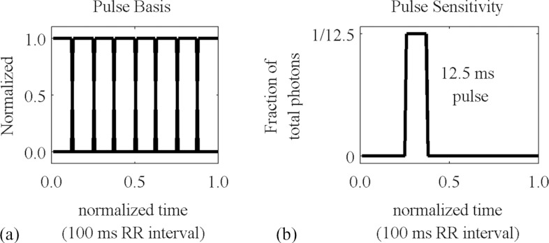
In the case of cyclical dynamic phenomena, such as the cardiac cycle or the respiratory cycle, we define t over the interval from 0 to 1 representing one complete period of the cycle, and the individual sensitivity and basis functions represent fractions of the cycle during which the projection is acquired and the image is reconstructed, respectively. In this study, both the temporal sensitivity and temporal basis functions are assumed to be rectangular pulses, but it is conceivable that other kinds of basis functions might be useful, such as triangles or sinusoids. Gaussian functions and gamma variate functions have been proposed for perfusion applications.21
Some of these basis functions and a typical temporal sensitivity function are shown in Fig. 6.
Figure 6.
Typical temporal basis functions and sensitivity function.
The same formula can include both temporal and spectral information:
| (14) |
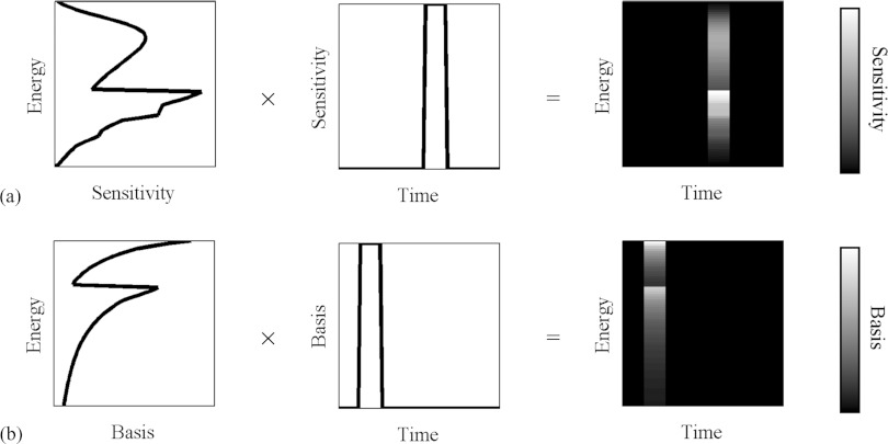
In this case, the sensitivity and basis functions are two-dimensional functions. Some of these functions are shown in Fig. 7. In this study, this is the formula that we use to find the expected photon counts at the detectors.
Figure 7.
Examples of spectral-temporal sensitivity functions (a) and basis functions (b). These functions are normalized and dimensionless.
To reconstruct images containing the values of the coefficients c at all voxels for all basis functions, we represent the quality of the reconstruction with cost functions K, we derive the gradients of these cost functions with respect to the coefficient of each basis function at each voxel, and we use the gradients to minimize the cost functions in an iterative fashion. To construct these gradients, we find the partial derivative of with respect to gradients, cjd:
| (15) |
where the function has been defined here for convenience. This equation is written with the arbitrary variable l that can represent energy, time, or a combination of the two.
The two cost functions we use are the data fidelity:
| (16) |
with the following gradient:
| (17) |
and the log-likelihood:
| (18) |
with the following gradient:
| (19) |
The two minimization techniques we use are gradient descent:
| (20) |
and fixed point iteration:
| (21) |
where the gradient of the cost function ∂K/∂cjd is represented as a difference of two components, ∂K1/∂cjd and ∂K2/∂cjd, such that ∂K/∂cjd = ∂K1/∂cjd − ∂K2/∂cjd, and the formulas of the gradients ∂K1/∂cjd and ∂K2/∂cjd can be readily determined by inspection of the formulas of the gradients of the cost functions. (For data fidelity, and , while for log-likelihood, and .) At each iteration n, these formulas take the estimate and use the gradient to construct an improved estimate . For both minimization techniques a relaxation factor α can be included to allow us to control the rate of convergence. It is not necessary to compute the expected photon counts at all the angles for which projections were acquired at every iteration; instead, different subsets of the angles can be used at each iteration. The number of subsets used at each iteration, the relaxation factor α, the cost function and the minimization technique constitute the main choices that must be made before performing iterative refinement. In general these parameters are scan-dependent.
The two algorithms based on gradient descent behave in a similar way, as do the two methods based on fixed point. To reduce the set of possible algorithms to explore, we have focused on data fidelity gradient descent (DFGD) and likelihood fixed point (LFP). In the conventional 3D CT realm, DFGD is the basis for the algebraic family of algorithms, such as the simultaneous algebraic reconstruction technique,22 while LFP is the basis for the statistical family of algorithms, such as the maximum likelihood algorithm.17 In our experience, LFP is more successful at adjusting the coefficient values to the correct range, while DFGD is more successful at establishing the proper boundaries between regions with different values. DFGD also tends to be less volatile and more amenable to the inclusion of filtration of the projections in order to accelerate convergence. Furthermore, formulas based on fixed point, such as LFP, will not change a voxel if its value before the update is 0. To balance the advantages and disadvantages of these two methods, we interleave DFGD and LFP, performing one iteration of one method followed by one iteration of the other.
Some algorithms developed by other groups based on LFP exploit the convexity of the formula in order to eliminate some terms and accelerate convergence.17 We have not used this approach, but we observe that such an approach is easily included in our model.
This algorithm does not make use of regularization or prior knowledge about the structure of the object, but such details could easily be included. We do make use of a non-negativity constraint at each iteration, and we perform the material decomposition at each iteration to force the concentrations to the correct range of values and prevent divergence.
Computation
In these formulas, the sum over voxels j from 1 to M for each pixel [Eqs. 10, 13, 14, 15] represents the forward projection function, while the sum over pixels i from 1 to N for each voxel [Eqs. 16, 17, 18, 19] represents the backprojection function, and these are the most computationally intensive steps in our algorithms. The reason is that the geometry term aij, the length of the portion of the x-ray trajectory from the x-ray source to pixel i that intersects voxel j, must be computed anew for every combination of voxels and pixels when these functions are called. In the live animal study in Sec. 3B, M = 640 × 640 × 100 = 4.1 × 10⁷ and N = 1002 × 300 × 3600 = 1.1 × 10⁹, meaning that an array of precomputed aij values would have M × N = 4.4 × 10¹⁶ elements, an impractically large number. Consequently, the forward projection and backprojection functions are the first priority in optimizing the reconstruction process for speed.
For the majority of combinations of i and j, aij has a value of 0, so dedicated array traversal and interpolation schemes are needed to avoid unnecessary computations. In our implementation, we use a ray-based scheme for forward projection, in which, for each pixel on the detector, we construct a ray from the source to the pixel, and then step along the array in constant increments through the volume, read the values at the points on the ray in the volume with trilinear interpolation, and sum all these values together. For backprojection we use a voxel-based scheme, in which, at each voxel, we perform a perspective transformation to find the corresponding detector pixels that fall on the ray from the source through the voxel, read the values from the projection with bilinear interpolation, and add these values to the voxel. Based on Zeng et al.,23 we do not believe that the use of two different schemes for backprojection and forward projection is a problem. To reduce computation time, we perform these operations on a graphics processing unit (GPU), using a GTX 285 (NVIDIA, Santa Clara, CA) programmed with CUDA. The GPU-based functions are accessed through a server that runs persistently in the background, enabling us to implement and test our reconstruction algorithms with MATLAB scripts, and reduce the number of memory transfers required during development.
Because of the linearity of the projection function, it is possible to move the linear combination of the basis functions at each voxel out of the projection, and instead compute a linear combination of projections:
| (22) |
If there are D basis functions defined over L points in time and energy, this replacement reduces the number of forward projection operations from L to D, which in our application is a difference of an order of magnitude.
The minimization techniques are expressed in terms of cjd, the coefficient at voxel j of basis function d. In updating these values at each iteration, we step through one basis function at a time and compute the values at all voxels. Each of these updates differ only by the term , but otherwise the computations are the same. Consequently, we can precompute the expected photon counts at each iteration, and use these values to update each volume without any additional forward projection operations. It is also possible to create the forward projections of each coefficient volume in advance at each iteration, but in our application there is insufficient memory to maintain all of these arrays.
Spectral model
As described in Secs. 2C, 2D, our method depends upon accurate knowledge of the spectral sensitivity of the imaging system. To predict the photon counts measured at the detector (or, in the case of our scintillation CCD detectors, the charge deposited at each pixel), we need to know how many photons are emitted at each x-ray energy, and the relative contribution of each photon (i.e., the chance of a signal being detected from an x-ray photon and the magnitude of this signal). The majority of this information is taken from the SPEKTR package,24 which includes results from prior studies of the emission spectra of x-ray tubes,25 and databases of elemental absorption spectra.26
Our spectral model is a sequence of several components. The x-rays are first generated by the collision of electrons on a tungsten anode in a vacuum tube, and the tungsten has a characteristic spectrum that is shaped by the voltage traversed by the electrons. These photons are subject to intrinsic filtration by the window on the tube, which is modeled as a given thickness of aluminum (0.7 mm) provided by the manufacturer (Varian Medical Systems, Palo Alto, CA). Additional filtration is provided by the metal filters placed outside the tube, and a 3 mm thick protective plate of plexiglass on the detector.
The remaining photons pass through a scintillator consisting of 0.025 g/cm2 gadolinium oxysulfide (Gd2O2S), and those x-ray photons that are absorbed produce a burst of optical photons. The number of optical photons produced by this process is directly proportional to the energy of the x-ray photons. This model of the detector is based on information provided by the manufacturer of our detectors (Photonic Science, East Sussex, UK).
The spectral sensitivity at a given energy is a product of the contributions of all of these components, and they can be combined into a single function:27
| (23) |
This sensitivity function is normalized so that the sum over all energies equals 1. The values of this function for our system are shown in Fig. 4. Before scanning the object, empty projections are collected (projections at each tube setting with no object present). The spectral sensitivity function for all pixels over all energies is the empty projection times the normalized sensitivity function. This implicitly assumes that the pixels on the detector differ only in the magnitude of their response, and not the spectra.
It is conceivable that any of the components described above might be improperly modeled, or there might be additional components outside the model that influence the spectral sensitivity. To account for possible mismatch between our model and the actual response of our system, we have developed a spectral calibration technique. This technique is presented in greater detail in Ref. 28, but we summarize it here.
A set of projections are collected in which various metal plates are placed between the tube and the detector. Equation 10 is used to find the expected number of measured photons predicted by our spectral model, and the discrepancy between the measured photon counts and the predicted photon counts is found. We then find a quadratic correction function that, when included in the spectral model, minimizes the difference between the measured counts and the predicted counts. This spectral calibration procedure reduces the average discrepancy between the measured counts and the predicted counts from 19% to 9%.
METHODS
We tested the utility of the various steps of our method (Fig. 1) in simulations (Sec. 3A). We then applied this method in in vivo scans of four mice (Sec. 3B).
Simulations
To test the utility of the steps of our technique, we used the Moby digital mouse phantom.29 This phantom is a volumetric representation of a mouse with optional respiratory and cardiac motion. We generated volumes at eight phases of the cardiac cycle without respiratory motion, and decomposed the volume into separate components for water and iodine, with 20 mg/ml iodine added to the blood. Vials containing water and 10 mg/ml iodine were attached to the phantom, as required by our technique. We simulated a scan of the phantom with retrospective gating, with each projection occurring at a randomly selected phase in the cardiac cycle. We generated 2400 projections with Eq. 14, with added Poisson noise. The noise levels in the projections were chosen so that the noise in reconstructions with conventionally distributed sets of projections were at the level we typically observe in studies with our micro-CT system, about 50 HU. The voltages and filters were chosen to match the settings described in the in vivo study in Sec. 3B, 41 kVp with a 0.1 mm tin filter in the low energy setting and 55 kVp with a 0.05 mm tungsten filter in the high energy setting.
The projections were interpolated to regularly spaced sets of 361 projections for each phase for each energy setting. For the bilateral filtration, we set σd = 1, σt = 1, and σr = 0.001 (attenuation coefficients, not HU). For the iterative refinement, we alternated between one iteration of DFGD with α = 0.25 and one iteration of LFP with α = 1, over 10 iterations total, with a randomly selected subset of 1/10 of the total projections at each iteration.
We use four metrics of image quality in order to evaluate the performance of the various steps of our method. The final goal of the material decomposition is to quantify the concentration of the iodine at each point in the object at each phase. We quantify the discrepancy between the true concentration and the reconstructed concentration at all points in the iodine volumes at all points in time with the root mean squared error (RMSE).
The vials included with the mouse have homogeneous interiors, and the vials are made of a homogeneous acrylic material with attenuation properties identical to water. In a perfect reconstruction, these regions should have a uniform value, but in practice the images are noisy, and the amount of noise is quantified by the standard deviation (STD) in these regions. In the steps of our method that produce attenuation images, this quantity is expressed in Hounsfield Units (HU), whereas in the steps that produce concentration images, this quantity is expressed in mg/ml.
However, some image processing techniques, such as simple convolutional smoothing, have the effect of blurring the image. This reduces the STD but, by making the boundaries between different materials diffuse and indistinct, diminishes image quality. Therefore, to quantify the sharpness of the boundaries in the image, we measure the modulation transfer function (MTF) at the boundary of one of the vials. To do this, we construct a series of line segments with one endpoint at the center of the vial and the other endpoint outside, with the exterior endpoints distributed in a circle around the vial, and we find the values in the image at regular intervals along these line segments with linear interpolation. This produces a set of radial profiles, which we average together. We then use a MATLAB curve-fitting function to fit a sigmoid function (based on the arctangent) to the average radial profile. This sigmoid function is the edge-spread function (ESF) of the image, the derivative of the ESF is the point-spread function (PSF), and the magnitude of the Fourier transform of the PSF is the MTF. The MTF is normalized so that the value at the 0 frequency is 1. We report a single value for the MTF: the spatial frequency at which it falls below 0.1. An ideal image should have a high MTF and a low STD. We measure these values around the vial containing water, since its boundary is more easily isolated.
To quantify our ability to accurately distinguish the chambers of the heart in order to compute various measures of cardiac function, we segment out the left ventricle, and compare the segmented region in the reconstructed images with the original phantom. The average number of misclassified voxels over all phases, expressed as a fraction of the total number of voxels in the region, is the segmentation error (SE). The segmentation technique entails finding and applying a threshold value halfway between the average values in the vials, applying morphological erosion to prevent spurious connections between the left and right ventricles, selecting the connected component that contains the left ventricle, and applying morphological dilation to recover the voxels lost by the erosion. This is not especially sophisticated, and it is not the same as the technique used in the in vivo study in Sec. 3B (which includes manual modifications to the segmented regions). We use this segmentation technique here to provide an objective and automated comparison of the contributions of the various stages of our method.
Live animal study
Our protocol is built around the unique capabilities and constraints of our custom dual source micro-CT system.30 X-rays are produced by two G-297 x-ray tubes (Varian Medical Systems, Palo Alto, CA) with 0.3/0.8 mm focal spots, powered by two Epsilon High Frequency x-ray generators (EMD Technologies, Quebec, Canada). The x-rays are detected by two XDI-VHR 2 CCD x-ray detectors (Photonic Science, East Sussex, UK) with a Gd2O2S phosphor and 22 μm pixels, which are typically binned to 88 μm. Each camera has a dedicated power supply, and a dedicated computer for image acquisition, but they receive the same acquisition trigger. The sources and detectors are stationary, and the animal is mounted vertically in a custom animal cradle and moved with an Oriel 13049 stepping motor (Newport, Stratford, CT) for rotation, on a stage that is operated with a separate Silverpak 17C stepping motor (Lin Engineering, Santa Clara, CA) for translation. Rotation and image acquisition are performed in step-and-shoot mode. The system is controlled by a dedicated program written in LabVIEW (National Instruments, Austin, TX).
Projections are acquired concurrently with each x-ray source at different energy settings. For each setting, the accelerating voltage, current, time, and filter must be chosen. We selected an optimal combination of voltages and filters in Sec. 2C. However, the combination of voltages and filters we use result in exposures with low flux, and the current and exposure time must be increased accordingly. These are limited by the heat capacity of the x-ray tubes and the desired temporal resolution.
In our protocol, we use the following energy settings:
Setting 1 (low energy): 41 kVp, 320 mA, 12.5 ms, 0.1 mm tin filter.
Setting 2 (high energy): 55 kVp, 400 mA, 12.5 ms, 0.05 mm tungsten filter.
The relative numbers of photons from the filtered tubes at each energy, scaled by the relative sensitivity of the detector, are shown in Fig. 4.
The currents are at the maximum allowed by our tubes but well below the amount that would saturate our detectors. The exposure times (12.5 ms) are determined by our desired temporal resolution, eight phases of the cardiac cycle in a mouse with ∼100 ms per heartbeat. Because of the heat capacity of the tubes, acquisitions must be broken into separate sets of projections, with several minutes between each set to allow the tubes to cool.
Changes in the orientation of the animal over the course of the scan, as well as imperfectly characterized geometry of our dual source system, may result in artifacts in the reconstructed images, such as double contours, streaks, and smears. These artifacts, which can hinder subsequent interpretation and processing, are often caused by a correlation between the rotation angle and the movement of the animal. By reducing this correlation we can reduce the artifacts, converting motion effects to an isotropic blur that is less disruptive to subsequent image processing and analysis. This strategy is motivated by similar techniques employed in radial sampling in MRI.31 We accomplish this reduction in correlation by interleaving the angles of the projections from each set, and alternating the settings of the two tubes. In other words, between each set, we switch the voltages and filters on the tubes, and we rotate the cradle by an angular offset. At the end of the entire scan, the acquired projections are sorted, resulting in a complete rotation for each tube setting with evenly distributed angles. The step angle and the total number of projections are limited by the desired scan time, radiation dose, and memory of the reconstruction engine.
We applied the proposed technique in in vivo scans of 4 C57BL/6 mice. This study was conducted under the protocol approved by the Duke University Institutional Animal Care and Use Committee. A liposomal blood pool contrast agent32 containing 123 mg I/ml was delivered by injection via a tail vein catheter at a dose of 0.01 ml/g body weight. Each animal was anesthetized with isoflurane (1.5%) mixed with 50% oxygen and balanced with nitrogen. ECG was monitored with electrodes taped to the footpads, and body temperature was maintained with heat lamps, a rectal probe, and feedback controller. A pneumatic pillow on the thorax was used to monitor respiration. Two vials, containing water and a 10 mg/ml iodine solution, were affixed to the cradle and scanned with the animal to facilitate the material decomposition.
Using the energy settings described above, a total of 3600 projections were acquired in 12 sets of 150 projections from 2 detectors. Each projection had 1002 × 667 pixels with a pitch of 0.088 mm × 0.088 mm. The step angle in each set was 1.2°, and an offset was introduced before each set so that the effective step angle for the entire experiment was 0.1°. After a few of the sets, we waited ∼5 min. for the tubes to cool. The total scan time was approximately 1 h. The estimated dose was 115 mGy.
We went through the reconstruction process with the two animals that had the largest and smallest variations in cardiac rate and respiratory rate (410–570 beats per minute [bpm] and 35–50 bpm respiratory rate in the former; 490–530 bpm and 30–39 bpm in the latter). We reconstructed the water and iodine components of the animals at eight phases of the cardiac cycle. Each volume was 640 × 640 × 100 voxels with a pitch of 0.110 mm × 0.110 mm × 0.110 mm. The projections were interpolated to regularly spaced sets of 361 projections for each phase for each energy setting for each camera. For the bilateral filtration, σd = 1.15, σt = 0.8, and σr = 0.002. For the iterative refinement, we used the same reconstruction algorithm as in the simulation.
At each phase in the iodine images, we segmented the left ventricle with Avizo (Visualization Sciences Group, Burlington, MA), and computed the volumes. The segmentation was performed by selecting a point in the ventricle, automatically finding the set of all points in the volume that were within a given range of iodine concentration values, identifying the connected component that contained the selected point, and then manually trimming away all the parts of this connected component that were located outside the ventricle. Using the maximum and minimum volumes in the left ventricle, we calculated the stroke volume, the ejection fraction, and the cardiac output.
RESULTS
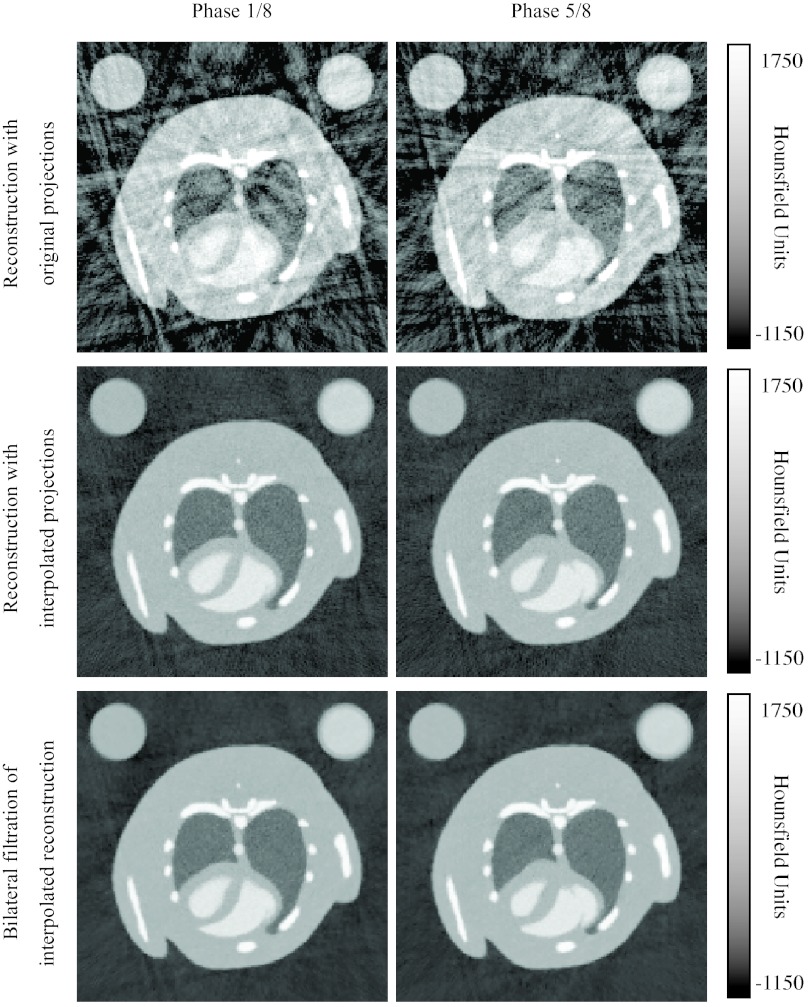
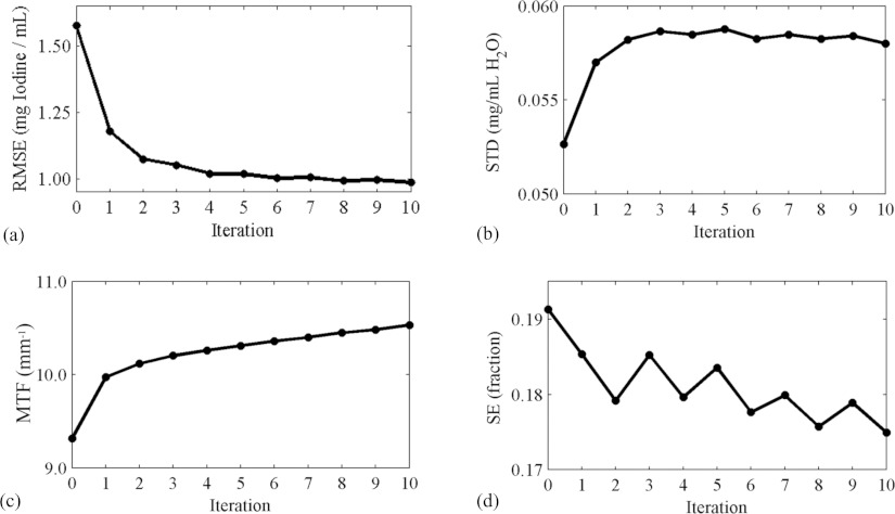
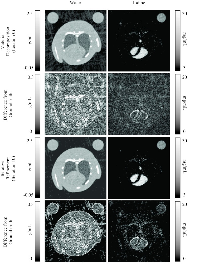
For the simulations, Table 1 shows the measured values of the RMSE, STD, MTF, and SE for reconstruction without projection interpolation (i.e., sorted projections), reconstruction with projection interpolation and bilateral filtration. Figure 8 shows some representative reconstructed images from the low energy setting at two phases in the cardiac cycle. The RMSE, STD, MTF, and SE values at each iteration are plotted in Fig. 9. Some concentration images are shown in Fig. 10.
Table 1.
Measurements of the reconstructed attenuation images from the simulation, with sorted projections and interpolated projections, without and with bilinear filtration.
| RMSE (mg iodine/ml) | STD (HU) | MTF at 0.1 (mm−1) | SE (fraction) | |
|---|---|---|---|---|
| Sorted projections | 58.6 | 130 | 7.9 | 0.24 |
| Interpolated projections | 2.7 | 44 | 6.4 | 0.14 |
| Bilinear filtration | 1.5 | 21 | 6.8 | 0.14 |
Figure 8.
Reconstructed attenuation images from the simulated scan using both original projections and interpolated projections, without and with bilateral filtration. Images with the low energy setting at two cardiac phases are shown.
Figure 9.
Measures of reconstruction quality at each iteration of the refinement process, starting with the result from the material decomposition (iteration 0): The RMSE of the estimated iodine concentration at all points in the iodine volumes at all points in time (a), the STD (b) and MTF (c) measured around the vial containing water, and the SE of the left ventricle (d).
Figure 10.
Images of the water and iodine components at one cardiac phase, before and after iterative refinement.
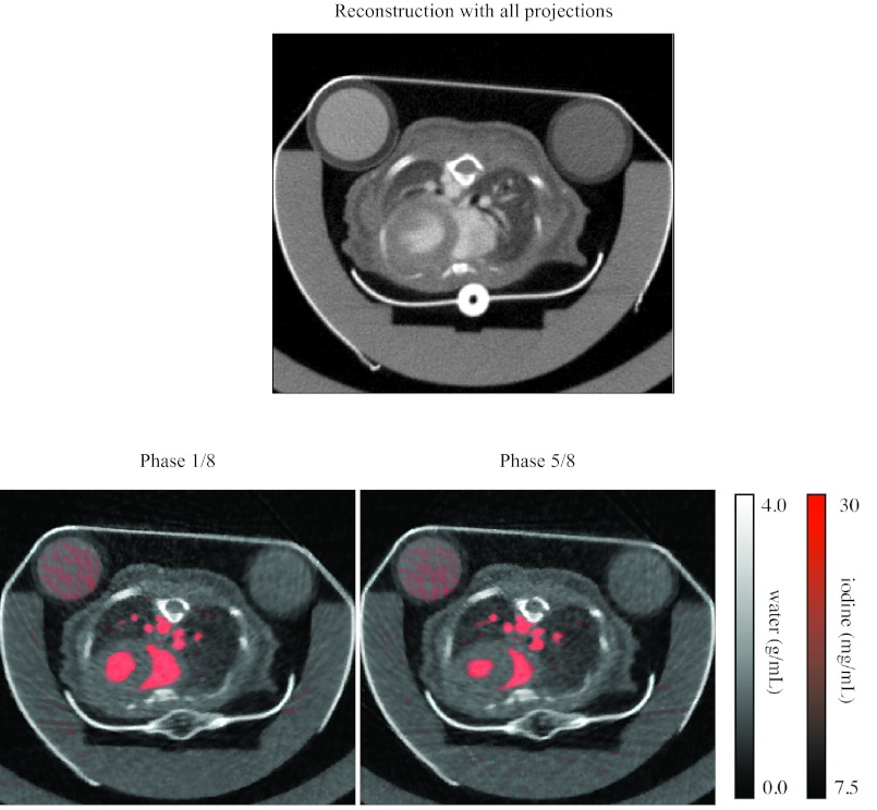
For the in vivo study, reconstructed images from one mouse are shown in Fig. 11. A time-averaged reconstruction with all the data from both tube settings is shown at the top, and images of the water and iodine components at two phases in the cardiac cycle are shown below. A closer view of a coronal section of the iodine in the heart over the cardiac cycle is shown in Fig. 12. Reconstruction time is reported in Table 2.
Figure 11.
Reconstructed images from the in vivo scan. An attenuation image reconstructed with all the projections is shown at the top. The material components at two cardiac phases are shown below, with water in grayscale and iodine in red.
Figure 12.

A closer view of a coronal section of the iodine in the heart over eight phases of the cardiac cycle, with the same color map as in Fig. 11.
Table 2.
Computation time of the steps of the reconstruction process for the in vivo study.
| Time (minutes) | |
|---|---|
| Projection interpolation | 11 |
| Filtered backprojection | 9 |
| Bilateral filtration | 3 |
| Material decomposition | 1 |
| Iterative refinement | 400 |
| Per iteration | 40 |
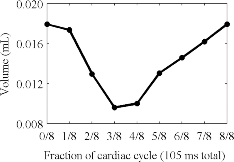
The volume of the segmented left ventricle of the heart of the mouse with the least variation in cardiac rate and respiratory rate is plotted in Fig. 13. For this mouse, the stroke volume was 0.0083 ml, and the ejection fraction was 46%. At a heart rate of 510 bpm, this corresponds to a cardiac output of 4.3 ml/min. For the mouse with the greatest variation, the stroke volume was 0.020 ml, and the ejection fraction was 43%. At a heart rate of 490 bpm, this corresponds to a cardiac output of 9.8 ml/min.
Figure 13.
The volume of the left ventricle of the heart over eight phases of the cardiac cycle, calculated from segmented images.
Animations of axial and coronal slices from the five-dimensional volume from one in vivo scan are available on our website.33 The thresholded iodine image is overlaid in red on the grayscale water image. The bone has been highlighted in blue by thresholding the water image and overlaying it on the grayscale water image. Additionally, we show an animated rendering of the segmented left ventricle superimposed on the grayscale iodine image. The five-dimensional volume is available for download.
DISCUSSION
Our technique is successful in distinguishing the distribution of iodine from the surrounding tissue (Figs. 101112). Large regions such as the heart with high concentrations of iodine can be discerned, and their motion is apparent (Fig. 12). The perspicuity of the iodinated regions makes it easier to segment them. The exact relationship between the reconstruction and the segmentation depends upon the kind of segmentation technique used. Our segmentation techniques, based on iodine concentration thresholds, benefit from the reduction in streaking artifacts and noise delivered by the projection interpolation (Table 1), while the iterative refinement reduces the error introduced by the material decomposition (Fig. 9). In the in vivo study, the calculated functional values (stroke volume, ejection fraction, and cardiac output) are within the range expected for a mouse, although the ejection fractions (43% and 46%) are rather low. This may be related to the nonzero SE associated with our method. It may indicate motion blur or incorrect segmentation of the walls of the ventricles in the reconstructed images, or it may indicate an abnormality in the mouse or the effects of the anesthetic. The substantial changes observed in the cardiac rate and the respiratory rate suggest that the heart motion may have been inconsistent over the course of the scan. In the mouse with the least variations in these rates, the ejection fraction is a little higher, but still somewhat out of the normal range. Further work is needed to establish the robustness of these measurements.
Our technique also succeeds in subtracting the iodine from the body, producing virtual pre-contrast images (Fig. 10). These images should be especially useful in studies where calcified plaques must be separated from iodinated blood, such as in imaging of atherosclerosis. In areas where the vessels lie close to the bone, the iodine and water images provide a clear distinction between the bone and the vessels that would be more difficult to distinguish on the basis of attenuation coefficients alone.
The simulations demonstrate the utility of the projection interpolation and bilateral filtration for improving the image quality of the reconstructions (Table 1). The reconstructed images are relatively free of the noise and streaking artifacts that typically accompany retrospective gating (Fig. 8) According to the MTF measurements, the projection interpolation slightly blurs the image, but this is compensated by a substantial reduction in noise. The bilateral filtration further reduces the noise while preserving the resolution.
Although the energy settings are optimized to facilitate the material decomposition (Fig. 4), the decomposition still has the effect of amplifying the noise, and some fine features are lost in the iodine concentration images.
The iterative refinement is successful in reducing the RMSE of the reconstruction (Fig. 9). Both the MTF and the STD are slightly increased, and the SE is decreased, suggesting that the image is sharpened. Most of the improvement occurs in the first four iterations, beyond which little change occurs. However, this improvement is rather slight, both quantitatively and visually (Fig. 10), and occurs mostly in the empty space surrounding the animal. Further work is needed to determine why this is so, but we speculate that there is too much overlap between the spectra of the different materials (Fig. 5), and between the spectral sensitivities at the different settings (Fig. 4). Even with the optimized voltages and filters, the values of water and iodine are still very close in attenuation space (Fig. 2). This situation might be improved by additional filtering of the x-ray spectra to produce narrower peaks around the K-edge, but this reduces the number of photons and increases the noise. To reduce the overlap of the basis functions, we have tried orthogonalizing them with QR decomposition, but this does not substantially affect performance.
The iterative refinement is less effective in the live animal scan. We suspect that there are additional factors in the image formation process that are not accounted for by our model and not fixed by spectral calibration. In particular, we do not account for x-ray scatter, a problem exacerbated by our dual source architecture in which both x-ray tubes fire simultaneously. In the presence of scatter, our estimate of , the expected number of photons at pixel i and energy e when no object is present, is no longer accurate. In our studies, when we fire one x-ray tube and acquire projection images from both detectors, the scattered signal measured at the detector that is not in line with the tube is typically ∼10% of the signal measured at the other detector, depending on the voltages and the object being scanned. In the future, this might be corrected by acquiring data from each tube at slightly different times, or by using more physically accurate methods to determine the expected number of photons.34
The computation times for most of the steps of the reconstruction (Table 2) are not problematic. However, the iterative refinement is especially time-consuming. Much of the time spent during this step takes place in the forward projection function, since we have insufficient memory to precompute the projections of all the basis functions. This problem may be overcome by using a computer with more memory (our computer has 24 GB of RAM).
Although we have focused on imaging iodine in the blood during the cardiac cycle, we believe that the strategy presented here can be extended to other studies of dynamic phenomena, such as perfusion,35 and other contrast materials, such as gadolinium36 or gold.37 It is possible to extend these techniques to include more than two energy settings and distinguish more than two materials, as long as the spectral properties of the materials are sufficiently distinct. (In our experience, calcium is not sufficiently distinct from water because of the absence of a K-edge in our energy range.) The data we have collected in this animal study can also be used to visualize and quantify respiration. Similar strategies can be used with other dual energy architectures.
This method requires the specification of values for several parameters which are dependent on the scanning protocol. The interpolation parameters should depend on the number of projections acquired and the number of phases to be reconstructed, which will in turn be influenced by dose and time considerations. The filtration parameters should depend on the desired resolution and the amount of noise in the unfiltered images, which depend on the results from the interpolation. The iterative refinement parameters should depend on the desired reconstruction time and the observed improvement. The values for the parameters that we used in the simulation and the live animal study were adjusted to optimize the final image quality for these particular scans. While our values may be good initial values for future studies, we expect that studies involving multiple scans and multiple animals on other imaging systems will adjust these values to optimize image quality in a test case, and then use the same values for all the scans in the study.
In conclusion, we have developed a technique for visualizing the changing distribution of iodine in the cardiac cycle with dual source micro-CT. This entails a retrospectively gated dual energy scan with optimized filters and voltages, and a series of computational operations to reconstruct the data and generate five-dimensional images. These images can be segmented, and the segmented images can be used to compute various measures of cardiac function, such as stroke volume, ejection fraction, and cardiac output. We believe this technique will be useful for future studies of cardiopulmonary disease in small animals.
ACKNOWLEDGMENTS
All work was performed at the Duke Center for In Vivo Microscopy, a NIH/NCRR/NIBIB National Biomedical Technology Research Center (P41 EB015897) with additional support from NCI (U24 CA092656). Liposomal contrast agent was provided by Ketan Ghaghada and Ananth Annapragada (Texas Childrens Hospital).
References
- Badea C. T. et al. , “In vivo small-animal imaging using micro-CT and digital subtraction angiography,” Phys. Med. Biol. 53(19), R319–R350 (2008). 10.1088/0031-9155/53/19/R01 [DOI] [PMC free article] [PubMed] [Google Scholar]
- Kachelriess M. et al. , “Kymogram detection and kymogram-correlated image reconstruction from subsecond spiral computed tomography scans of the heart,”Med. Phys. 29(7), 1489–1504 (2002). 10.1118/1.1487861 [DOI] [PubMed] [Google Scholar]
- Bartling S. H. et al. , “Retrospective motion gating in small animal CT of mice and rats,” Invest. Radiol. 42(10), 704–714 (2007). 10.1097/RLI.0b013e318070dcad [DOI] [PubMed] [Google Scholar]
- Badea C. T. et al. , “4-D micro-CT of the mouse heart,” Mol. Imaging 4(2), 110–116 (2005). [DOI] [PubMed] [Google Scholar]
- Drangova M. et al. , “Fast retrospectively gated quantitative four-dimensional (4D) cardiac micro computed tomography imaging of free-breathing mice,” Invest. Radiol. 42(2), 85–94 (2007). 10.1097/01.rli.0000251572.56139.a3 [DOI] [PubMed] [Google Scholar]
- Song J. et al. , “Sparseness prior based iterative image reconstruction for retrospectively gated cardiac micro-CT,” Med. Phys. 34, 4476–4483 (2007). 10.1118/1.2795830 [DOI] [PMC free article] [PubMed] [Google Scholar]
- Chen G. H., Tang J., and Leng S. H., “Prior image constrained compressed sensing (PICCS): A method to accurately reconstruct dynamic CT images from highly undersampled projection data sets,” Med. Phys. 35(2), 660–663 (2008). 10.1118/1.2836423 [DOI] [PMC free article] [PubMed] [Google Scholar]
- Sawall S. et al. , “Low-dose cardio-respiratory phase-correlated cone-beam micro-CT of small animals,” Med. Phys. 38(3), 1416–1424 (2011). 10.1118/1.3551993 [DOI] [PubMed] [Google Scholar]
- Alvarez R. E. and Macovski A., “Energy-selective reconstructions in x-ray computerized tomography,” Phys. Med. Biol. 21(5), 733–744 (1976). 10.1088/0031-9155/21/5/002 [DOI] [PubMed] [Google Scholar]
- Taschereau R., Silverman R. W., and Chatziioannou A. F., “Dual-energy attenuation coefficient decomposition with differential filtration and application to a micro-CT scanner,” Phys. Med. Biology 55(4), 1141–1155 (2010). 10.1088/0031-9155/55/4/016 [DOI] [PMC free article] [PubMed] [Google Scholar]
- Huh W. and Fessler J. A., “Model-based image reconstruction for dual-energy x-ray CT with fast Kvp switching,” IEEE International Symposium on Biomedical Imaging (IEEE, New York, 2009), pp. 326–329.
- Flohr T. G. et al. , “First performance evaluation of a dual-source CT (DSCT) system,” Eur. Radiol. 16(2), 256–268 (2006). 10.1007/s00330-005-2919-2 [DOI] [PubMed] [Google Scholar]
- Heismann B. J. and Wirth S., “SNR performance comparison of dual-layer detector and dual-kVp spectral CT,” Nuclear Science Symposium Conference Record (IEEE Medical Imaging Conference Record, pp. 3280–3822, Honolulu, HI, 2007).
- Granton P. V. et al. , “Implementation of dual- and triple-energy cone-beam micro-CT for postreconstruction material decomposition,” Med. Phys. 35(11), 5030–5042 (2008). 10.1118/1.2987668 [DOI] [PubMed] [Google Scholar]
- Chueh H. S. et al. , “Development of novel statistical reconstruction algorithms for poly-energetic X-ray computed tomography,” Comput. Methods Programs Biomed. 92(3), 289–293 (2008). 10.1016/j.cmpb.2008.04.002 [DOI] [PubMed] [Google Scholar]
- Elbakri I. A. and Fessler J. A., “Statistical image reconstruction for polyenergetic x-ray computed tomography,” IEEE Trans. Med. Imaging 21(2), 89–99 (2002). 10.1109/42.993128 [DOI] [PubMed] [Google Scholar]
- Erdogan H. and Fessler J. A., “Monotonic algorithms for transmission tomography,” IEEE Trans. Med. Imaging 18(9), 801–814 (1999). 10.1109/42.802758 [DOI] [PubMed] [Google Scholar]
- Feldkamp L. A., Davis L. C., and Kress J. W., “Practical cone-beam algorithm,” J. Opt. Soc. Am. A Opt. Image Sci. Vis 1(6), 612–619 (1984). 10.1364/JOSAA.1.000612 [DOI] [Google Scholar]
- Tomasi C. and Manduchi R., “Bilateral filtering for gray and color images,” Proceedings of the 1998 IEEE International Conference on Computer Vision (1998), pp. 839–846.
- Press W. H.et al. Numerical Recipes, 3rd ed. (Cambridge University Press, Cambridge, England, 2007). [Google Scholar]
- Neukirchen C., Giordano M., and Wiesner S., “An iterative method for tomographic x-ray perfusion estimation in a decomposition model-based approach,” Med. Phys. 37(12), 6125–6141 (2010). 10.1118/1.3495818 [DOI] [PubMed] [Google Scholar]
- Andersen A. H. and Kak A. C., “Simultaneous algebraic reconstruction technique (SART): A superior implementation of the ART algorithm,” Ultrason. Imaging 6(1), 81–94 (1984). 10.1016/0161-7346(84)90008-7 [DOI] [PubMed] [Google Scholar]
- Zeng G. S. L. and Gullberg G. T., “Unmatched projector/backprojector pairs in an iterative reconstruction algorithm,” IEEE Trans. Med. Imaging 19(5), 548–555 (2000). 10.1109/42.870265 [DOI] [PMC free article] [PubMed] [Google Scholar]
- Siewerdsen J. H. et al. , “Spektr: A computational tool for x-ray spectral analysis and imaging system optimization,” Med. Phys. 31(11), 3057–3067 (2004). 10.1118/1.1758350 [DOI] [PubMed] [Google Scholar]
- Boone J. M. and Seibert J. A., “Accurate method for computer-generating tungsten anode x-ray spectra from 30 to 140 kV,” Med. Phys. 24(11), 1661–1670 (1997). 10.1118/1.597953 [DOI] [PubMed] [Google Scholar]
- Hubbell J. H. et al. , “A review, bibliography, and tabulation of K, L, and higher atomic shell x-ray-fluorescence yields,” J. Phys. Chem. Ref. Data 23(2), 339–364 (1994). 10.1063/1.555955 [DOI] [Google Scholar]
- Heismann B. and Balda M., “Quantitative image-based spectral reconstruction for computed tomography,” Med. Phys. 36(10), 4471–4485 (2009). 10.1118/1.3213534 [DOI] [PubMed] [Google Scholar]
- Johnston S. M., Johnson G. A., and Badea C. T., “A spectral calibration technique for x-ray CT,” Proc. SPIE 8313, 831333 (2012). 10.1117/12.911532 [DOI] [Google Scholar]
- Segars W. P. et al. , “Development of a 4-D digital mouse phantom for molecular imaging research,” Mol. Imaging Biol. 6(3), 149–159 (2004). 10.1016/j.mibio.2004.03.002 [DOI] [PubMed] [Google Scholar]
- Badea C. T. et al. , “A dual micro-CT system for small animal imaging,” Proc. SPIE 6913, 691342 (2008). 10.1117/12.772303 [DOI] [PMC free article] [PubMed] [Google Scholar]
- Winkelmann S. et al. , “An optimal radial profile order based on the golden ratio for time-resolved MRI,” IEEE Trans. Med. Imaging 26(1), 68–76 (2007). 10.1109/TMI.2006.885337 [DOI] [PubMed] [Google Scholar]
- Ghaghada K. B. et al. , “Evaluation of tumor microenvironment in an Animal model using a nanoparticle contrast agent in computed tomography imaging,” Acad. Radiol. 18(1), 20–30 (2011). 10.1016/j.acra.2010.09.003 [DOI] [PMC free article] [PubMed] [Google Scholar]
- www.civm.duhs.duke.edu/medphy5dct/.
- Taschereau R., Chow P. L., and Chatziioannou A. F., “Monte Carlo simulations of dose from microCT imaging procedures in a realistic mouse phantom,” Med. Phys. 33(1), 216–224 (2006). 10.1118/1.2148333 [DOI] [PMC free article] [PubMed] [Google Scholar]
- Badea C. T. et al. , “Lung perfusion imaging in small animals using 4D micro-CT at heartbeat temporal resolution,” Med. Phys. 37(1), 54–62 (2010). 10.1118/1.3264619 [DOI] [PMC free article] [PubMed] [Google Scholar]
- Gierada D. S. and Kyongtae T. B., “Gadolinium as a CT contrast agent: Assessment in a porcine model,” Radiology 210(3), 829–834 (1999). [DOI] [PubMed] [Google Scholar]
- Badea C. T. et al. , “Dual-energy micro-CT imaging for differentiation of iodine- and gold-based nanoparticles temporal and spectral reconstruction algorithms for x-ray CT,” Proc. SPIE 7961, 79611X (2011). 10.1117/12.878043 [DOI] [Google Scholar]


