Comparison of image registration based measures of regional lung ventilation from dynamic spiral CT with Xe-CT

Abstract

Purpose: Regional lung volume change as a function of lung inflation serves as an index of parenchymal and airway status as well as an index of regional ventilation and can be used to detect pathologic changes over time. In this paper, the authors propose a new regional measure of lung mechanics—the specific air volume change by corrected Jacobian. The authors compare this new measure, along with two existing registration based measures of lung ventilation, to a regional ventilation measurement derived from xenon-CT (Xe-CT) imaging.

Methods: 4DCT and Xe-CT datasets from four adult sheep are used in this study. Nonlinear, 3D image registration is applied to register an image acquired near end inspiration to an image acquired near end expiration. Approximately 200 annotated anatomical points are used as landmarks to evaluate registration accuracy. Three different registration based measures of regional lung mechanics are derived and compared: the specific air volume change calculated from the Jacobian (SAJ); the specific air volume change calculated by the corrected Jacobian (SACJ); and the specific air volume change by intensity change (SAI). The authors show that the commonly used SAI measure can be derived from the direct SAJ measure by using the air-tissue mixture model and assuming there is no tissue volume change between the end inspiration and end expiration datasets. All three ventilation measures are evaluated by comparing to Xe-CT estimates of regional ventilation.

Results: After registration, the mean registration error is on the order of 1 mm. For cubical regions of interest (ROIs) in cubes with size 20 mm × 20 mm × 20 mm, the SAJ and SACJ measures show significantly higher correlation (linear regression, average r² = 0.75 and r² = 0.82) with the Xe-CT based measure of specific ventilation (sV) than the SAI measure. For ROIs in slabs along the ventral-dorsal vertical direction with size of 150 mm × 8 mm × 40 mm, the SAJ, SACJ, and SAI all show high correlation (linear regression, average r² = 0.88, r² = 0.92, and r² = 0.87) with the Xe-CT based sV without significant differences when comparing between the three methods. The authors demonstrate a linear relationship between the difference of specific air volume change and difference of tissue volume in all four animals (linear regression, average r² = 0.86).

Conclusions: Given a deformation field by an image registration algorithm, significant differences between the SAJ, SACJ, and SAI measures were found at a regional level compared to the Xe-CT sV in four sheep that were studied. The SACJ introduced here, provides better correlations with Xe-CT based sV than the SAJ and SAI measures, thus providing an improved surrogate for regional ventilation.

INTRODUCTION

Regional ventilation is the term used to characterize the volume of fresh gas per unit time that enters or exits the lung at the acinar (gas exchange) level. Disruption of regional ventilation can reflect alterations to airways (physiological or pathological), alterations in parenchymal mechanics, changes to the muscles of respiration, body posture effects, and inhaled gas properties. Thus, measures of regional lung mechanics can serve as a sensitive test of the status of the respiratory system and should be considerably more sensitive and informative than global pulmonary function test. Recent advances in multidetector-row CT (MDCT), 4DCT respiratory gating methods, and image processing techniques enable us to study pulmonary function at the regional level with high resolution anatomical information compared to other methods. MDCT can be used to acquire multiple static breath-hold CT images of the lung taken at different lung volumes, or 4DCT images of the lung acquired during spiral scanning using a low pitch and retrospectively reconstructed at different respiratory phases with proper respiratory control.^{1, 2, 3} Image registration can be applied to these data to estimate a deformation field that transforms the lung from one volume configuration to the other. This deformation field can be analyzed to estimate local lung tissue expansion, calculate voxel-by-voxel intensity change, and make biomechanical measurements. When combined with image segmentation algorithms,^{4, 5, 6, 7} functional and biomechanical measurements can be reported on a lung, lobe, and sublobar basis, and can be used to interpret regional lung function relative to specific segments of bronchial tree. Such measurements of pulmonary function have proven useful as a planning tool during RT planning^{8, 9} and may be useful for tracking the progression of toxicity to nearby normal tissue during RT and can be used to evaluate the effectiveness of a treatment posttherapy.¹⁰

Early studies using CT to study regional air volume changes have proved to enhance our understanding of normal lung function. Several groups have proposed methods that couple image registration and CT imaging to study regional lung function. Guerrero etal. have used optical-flow registration to compute lung ventilation from 4DCT (Refs. ^{11, 12}) with an intensity-based ventilation measure. Christensen et al. used image registration to match images across cine-CT sequences and estimate rates of local tissue expansion and contraction¹³ using a Jacobian-based ventilation measure. While they were able to show that their accumulated measurements matched well with the global measurements, they were not able to compare the registration based measurements to local measures of regional tissue ventilation. Recently, Castillo et al. compared the intensity-based and Jacobian-based calculations of ventilation from 4DCT with the ventilation from ^99mTc-labeled aerosol SPECT/CT.¹⁴ A statistically higher correlation to the SPECT/CT based ventilation was found for intensity-based calculation over the Jacobian-based calculation. However, the comparison of the two techniques was based on the Dice similarity coefficient between the thresholded masks within 20% variation from the 4DCT and from SPECT/CT. Though their experiment is novel and important, since the average mask size is about 490.5 mL (with average subject exhale volume 2452.7 mL, and five submasks per subject), the comparison is more global than regional. In addition, as shown in Sec. 2D, both the intensity-based and Jacobian-based ventilation measures are based on the assumption that regional lung volume change is due solely to air content change, which may not always be a valid assumption. Other factors, such as blood volume change, may also introduce the regional lung volume change.

The physiologic significance of these registration based measures of respiratory function can be established by comparing to more conventional measurements, such as nuclear medicine or contrast wash-in/wash-out studies with CT or MR. Xenon-enhanced CT (Xe-CT) measures regional ventilation by observing the gas wash-in or wash-out rate on serial CT images.^{15, 16, 17} Xe-CT imaging has the advantage of high temporal resolution and spatial resolution and reflects a measure of fresh gas delivery to the gas exchange units of the lung. Although the dynamic Xe-CT method is limited in Z-axis coverage, requires expensive Xe gas, and is technically challenging, it serves as the gold standard of regional ventilation and can be used to compare with registration based measures of regional lung function in animal studies for validation purposes.

This paper describes three measures to estimate regional ventilation from image registration of CT images: the specific air volume change calculated from the Jacobian (SAJ); the specific air volume change calculated by the corrected Jacobian (SACJ); and the specific air volume change by intensity change (SAI). We show that the SAI ventilation measure can be derived from the SAJ measure by making the assumption that there is no tissue volume change between registration volumes. We evaluate these three measures by comparing them with a Xe-CT measure of ventilation in a regional basis (20 mm × 20 mm × 20 mm cube, or 8 mL). Among these three registration based measures, we show that the corrected Jacobian-based measure, SACJ, has the best correlation with the Xe-CT derived measure of specific ventilation.

MATERIAL AND METHODS

Method overview

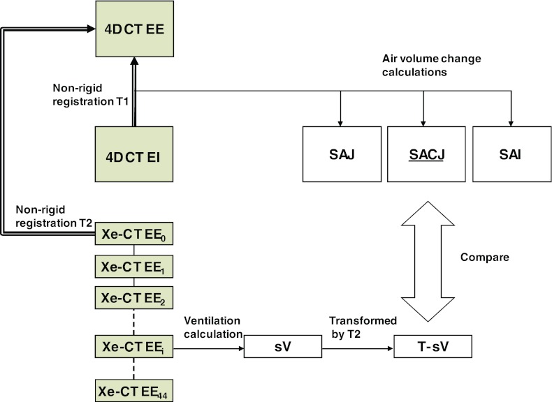
Our goal is to validate and compare the measures used to estimate regional lung ventilation from image registration by comparing them to Xe-CT estimated ventilation. Figure 1 shows a block diagram of the entire process. Two types of data were acquired for each animal: a 4DCT scan and a Xe-CT scan. In order to make our comparisons under the same physiological conditions, each animal was scanned and mechanically ventilated with the same respiratory rate, tidal volume (TV) and positive end-expiratory pressure (PEEP) during the two types of scans. The datasets from the 4DCT scan were reconstructed in volumes at eight phases of the respiratory cycle. For this study we focus on the datasets from two of the phases, a volume near end expiration (EE) and a volume near end inspiration (EI). For the Xe-CT scan, 45 distinctive partial lung volumetric scans were performed at volume near end expiration, or the initial end expiration scan (EE₀) to the last expiration scan (EE₄₄).

Figure 1.

Figure shows the two types of images, an image pair of full lung volumetric phases EE and EI from a 4DCT scan and a Xe-CT scan acquired at the end of expiration over 45 respiratory cycles (EE₀ to EE₄₄), which are analyzed during the processing. Transformation T1 registers EI to EE data and can be used to assess local lung function via calculations of three ventilation measures: SAJ, SACJ, and SAI. The 45 distinctive partial lung volumetric Xe-CT scans EE₀ to EE₄₄ are used to calculate Xe-CT based measure of sV. Transformation T2 maps the sV data into the coordinate system of the EE image (end expiration phase of the 4DCT scan) to allow direct comparison with the 4DCT and registration based measures of ventilation. Both EE and EE₀ are at volumes near end inspiration. (Shaded boxes indicate CT image data; white boxes indicated derived or calculated data; thick arrows indicate image registration transformations being calculated; thin solid lines indicate other operations.)

The nonlinear image registration is used to define the transformation T1 between the EE and EI in order to measure the regional lung ventilation from the 4DCT scan. The Xe-CT based estimated regional lung ventilation is computed on the EE₀ by using Pulmonary Analysis Software Suite 11.0 (PASS) software by finding the constant of the exponential rise of the density from xenon gas wash-in over multiple breaths.¹⁸ The same nonlinear image registration is also applied to define the transformation T2 which maps the EE₀ to the EE so that the Xe-CT based estimate of ventilation can be mapped into the same coordinate system as that of the registration based estimate of ventilation. Additional details on the registration algorithm and other processing steps are given below.

Image datasets

Appropriate animal ethics approval was obtained for these protocols from the University of Iowa Animal Care and Use Committee and the study adhered to NIH guidelines for animal experimentation. Four adult male sheep A, B, C, and D (with weights 44.0, 37.8, 40.4, and 46.7 kg) were used for this study. The sheep were anesthetized using intravenous pentobarbital and pancuronium to ensure adequate sedation and to prevent spontaneous breathing. Animals were positive pressure ventilated during experiments using a custom built dual Harvard apparatus piston ventilator designed for computer control. The 4DCT images were acquired with the animals in the supine position using the dynamic imaging protocol with a pitch of 0.1, slice collimation of 0.6 mm, rotation time of 0.5 s, slice thickness of 0.75 mm, slice increment of 0.5 mm, 120 kV, 400 mAs, and kernel B30f. The airway pressure signal was simultaneously recorded with the x-ray projections and images were reconstructed retrospectively at 0%, 25%, 50%, 75%, and 100% of the inspiration duration and 75%, 50%, and 25% of the expiration duration. The 0% (EE) and 100% (EI) inspiration phases were used for later ventilation measurements. A slab of 12 contiguous axial slices were imaged over 45 breaths for Xe-CT scans. Images were acquired using respiratory gating by triggering the scan during end-expiration with 80 keV energy (for higher density resolution, approximately 2 HU per 1% Xe), 160 mAs tube current, a 360° rotation, a 0.33 s scan time, and 2.4 mm slice thickness. Respiratory gating is achieved using a custom built LabVIEW program which controls the ventilators and triggers the CT scanner. The respiratory rate (RR) for four animals ranged from 15 to 18 breaths per minute with an inspiratory-expiratory ratio of 1:1 which was sufficient to maintain a normocapnic state. Both of the two types of images were acquired with a matrix of 512 by 512 and without moving the animal between scans.

Image registration

A tissue volume and vesselness measure preserving nonrigid registration (TVP) algorithm^{19, 20} is used to estimate the transformations EI to EE and EE₀ to EE. The TVP algorithm minimizes the sum of squared tissue volume difference (SSTVD) (Refs. ^{21, 22, 23, 24} and vesselness measure difference (SSVMD), utilizing the rich image intensity information and natural anatomic landmarks provided by the vessels. This method has been shown to be effective at registering across lung CT images with high accuracy.^{19, 20}

Let I₁ and I₂ represent two 3D image volumes to be registered. The vector x = (x₁, x₂, x₃)^T defines the voxel coordinate within an image. The algorithm finds the optimal transformation h that maps the template image I₁ to the target image I₂ by minimizing the cost function,

$$\begin{array}{ccc}\hfill C_{\text{TOTAL}}& =& \rho {\int }_{\Omega }{\left[V_2\left(\mathbf{x}\right)-V_1\left(\mathbf{h}\left(\mathbf{x}\right)\right)\right]}^{2}d\mathbf{x}\hfill \\ & & +\chi {\int }_{\Omega }{\left[F_2\left(\mathbf{x}\right)-F_1\left(\mathbf{h}\left(\mathbf{x}\right)\right)\right]}^{2}d\mathbf{x},\hfill \end{array}$$ (1)

where Ω is the union domain of the lung regions in images I₁ and I₂. V₂ and V₁ are the tissue volumes as defined in Eq. 2. F₂ and F₁ are the vesselness measures as defined in Eq. 6. The transformation h is a (3 × 1) vector-valued function that maps a point h(x) in the target image to its corresponding location in the template image. The first integral of the cost function defines the SSTVD cost and the second integral of the cost function defines the SSVMD cost. In the following part, we first introduce SSTVD in Eqs. 2– 5 and then we introduce SSVMD in Eqs. 6, 7.

The SSTVD cost assumes that the measured Hounsfield unit (HU) in the lung CT images is a function of tissue and air content. Following the air-tissue mixture model by Hoffman and Ritman²⁵ from the CT value of a given voxel, the tissue volume can be estimated as

$$V\left(\mathbf{x}\right)=\nu \left(\mathbf{x}\right)\frac{I\left(\mathbf{x}\right)-{\text{HU}}_{\text{air}}}{{\text{HU}}_{\text{tissue}}-{\text{HU}}_{\text{air}}}=\nu \left(\mathbf{x}\right)\beta \left(I\left(\mathbf{x}\right)\right),$$ (2)

and the air volume can be estimated as

$$V^{\prime }\left(\mathbf{x}\right)=\nu \left(\mathbf{x}\right)\frac{{\text{HU}}_{\text{tissue}}-I\left(\mathbf{x}\right)}{{\text{HU}}_{\text{tissue}}-{\text{HU}}_{\text{air}}}=\nu \left(\mathbf{x}\right)\alpha \left(I\left(\mathbf{x}\right)\right),$$ (3)

where ν(x) denotes the volume of voxel x and I(x) is the intensity of a voxel at position x. HU_air and HU_tissue refer to the intensity of air and tissue, respectively. In this work, we assume that air is −1000 HU and tissue is 0 HU. $\alpha \left(I\left(\mathbf{x}\right)\right)=\frac{{\text{HU}}_{\text{tissue}}-I\left(\mathbf{x}\right)}{{\text{HU}}_{tissue}-{\text{HU}}_{air}}$ and $\beta \left(I\left(\mathbf{x}\right)\right)=\frac{I\left(\mathbf{x}\right)-{\text{HU}}_{\text{air}}}{{\text{HU}}_{\text{tissue}}-{\text{HU}}_{\text{air}}}$ are introduced for notational simplicity. Notice that α(I(x)) + β(I(x)) = 1.

Given 2, we can then define the SSTVD cost:

$$\begin{array}{c}\hfill C_{\text{SSTVD}}={\int }_{\Omega }{\left[V_2\left(\mathbf{x}\right)-V_1\left(\mathbf{h}\left(\mathbf{x}\right)\right)\right]}^{2}d\mathbf{x}\end{array}$$ (4)

$$\begin{array}{c}\hfill ={\int }_{\Omega }{\left[{\nu }_2\left(\mathbf{x}\right)\beta \left(I_2\left(\mathbf{x}\right)\right)-{\nu }_1\left(\mathbf{h}\left(\mathbf{x}\right)\right)\beta \left(I_1\left(\mathbf{h}\left(\mathbf{x}\right)\right)\right)\right]}^{2}d\mathbf{x}.\end{array}$$ (5)

The notation I₁(h(x)) is interpreted as the image I₁(x) deformed by the transformation h(x) and is computed using trilinear interpolation. The deformed volume element ν₁(h(x)) is calculated using the Jacobian J(x) times the volume element ν₂(x), i.e., ν₁(h(x)) = J(x)ν₂(x).

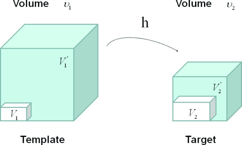
Figure 2 shows an example of a cubic shaped region under deformation h from template image to target image. The region volumes are ν₁ and ν₂. The volumes can be decomposed into the tissue volume fraction and air volume fraction based on the mean voxel intensity within the cube. The small white subvolumes inside the cubes represent the tissue volume V₁ and V₂. Air volumes are represented by $V_1^{\prime }$ and $V_2^{\prime }$ (in blue). As the ratio of air to tissue decreases, the CT intensity of a voxel increases. The mean cube voxel intensities for the template, I₁, and target images, I₂, are functions of the ratios of air to tissue volumes within the cubes.

Figure 2.

Example of a region under deformation h(x) from template image to target image. V₁ and V₂ are tissue volumes in the regions. $V_1^{\prime }$ and $V_2^{\prime }$ are air volumes in the regions. Region volumes ${\nu }_1=V_1+V_1^{\prime }$ and ${\nu }_2=V_2+V_2^{\prime }$.

As the blood vessels branch to smaller and smaller diameters, the raw gray scale information from vessel voxels provide very little contribution to guide the intensity-based registration. To better utilize the information of blood vessel locations, we use the vesselness measure based on the eigenvalues of the Hessian matrix of image intensity. Frangi's vesselness function²⁶ is defined as

$$\begin{array}{ccc}& & F\left(\lambda \right)\hfill \\ & & =\left\{\begin{array}{cc}(1-e^{-\frac{R_A^2}{2{\alpha }^2}})·e^{\frac{-R_B^2}{2{\beta }^2}}·(1-e^{-\frac{S^2}{2{\gamma }^2}})\hfill & \text{if}{\lambda }_2<0\text{and}{\lambda }_3<0\hfill \\ 0\hfill & \text{otherwise}\hfill \end{array}\right.,\hfill \end{array}$$ (6)

with

$$R_A=\frac{|{\lambda }_2|}{|{\lambda }_3|},R_B=\frac{|{\lambda }_1|}{\sqrt{|{\lambda }_2{\lambda }_3|}},S=\sqrt{{\lambda }_1^2+{\lambda }_2^2+{\lambda }_3^2},$$ (7)

where R_A distinguishes between platelike and tubular structures, R_B accounts for the deviation from a bloblike structure, and S differentiates between tubular structure and noise. The vesselness function has been previously widely used in vessel segmentations in lungs^{27, 28} and in retinas.²⁹ α, β, γ control the sensitivity of the vesselness measure. The vesselness measure is rescaled to [0, 1] and can be considered as a probabilitylike estimate of vesselness features. For this study, α = 0.5, β = 0.5, and γ = 5 and the weighting constants in the total cost were set as ρ = 1 and χ = 0.2. These parameters are similar to those used in our previous work.^{19, 20}

The transformation h(x) is a cubic B-splines transform:

$$\mathbf{h}\left(\mathbf{x}\right)=\mathbf{x}+\sum _{i\in G}{\varphi }_i{\beta }^{\left(3\right)}(\mathbf{x}-{\mathbf{x}}_i),$$ (8)

where ϕ_i describes the displacements of the control nodes and β⁽³⁾(x) is a three-dimensional tensor product of basis functions of cubic B-Spline. A spatial multiresolution procedure from coarse to fine is used in the registration in order to improve speed, accuracy, and robustness. The total cost in Eq. 1 is optimized using a limited-memory, quasi-Newton minimization method with bounds (L-BFGS-B) (Ref. ³⁰) algorithm. The B-splines coefficients are constrained so that the transformation maintains the topology using the sufficient conditions that guarantee the local injectivity of functions parameterized by uniform cubic B-splines proposed by Choi and Lee.³¹

Regional ventilation measures from image registration

After we obtain the optimal warping function h(x), we can calculate the regional ventilation, which is equal to the difference in local air volume change per unit time. The commonly used ventilation measure is the specific ventilation sV which takes the initial air volume into account. The sV is equal to the specific air volume change sVol per unit time. Or in other words, in a unit time,

$$\text{sV}=\text{sVol}=\frac{V_1^{\prime }\left(\mathbf{h}\left(\mathbf{x}\right)\right)-V_2^{\prime }\left(\mathbf{x}\right)}{V_2^{\prime }\left(\mathbf{x}\right)}.$$ (9)

Three different approaches for estimating 9 are described below:

Specific air volume change by specific volume change (SAJ):

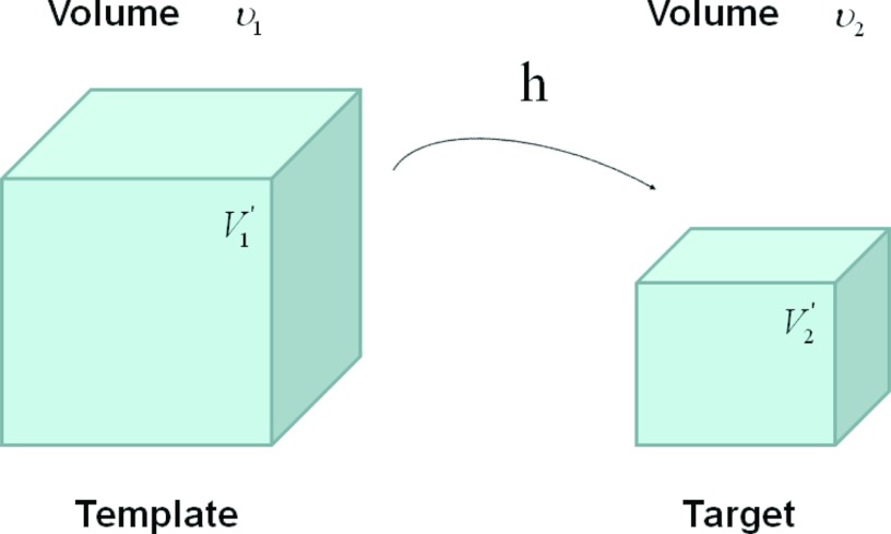
The SAJ regional ventilation measure is based on the assumption that there is no tissue volume within the template or target volumes, and thus any local air volume change is equal to the local volume change. Figure 3 illustrates such an assumption. Compared with the general condition in Fig. 2, the region volume now is pure air volume, or equivalently, ${\nu }_1=V_1^{\prime }$ and ${\nu }_2=V_2^{\prime }$. In this case, the specific air volume change is equal to specific volume change. Since the Jacobian tells us the local volume expansion (or contraction), the regional ventilation can be measured by

$$\text{SAJ}=\frac{{\nu }_1\left(\mathbf{h}\left(\mathbf{x}\right)\right)-{\nu }_2\left(\mathbf{x}\right)}{{\nu }_2\left(\mathbf{x}\right)}=J\left(\mathbf{x}\right)-1.$$ (10)

Previously, SAJ has been used as an index of the regional function and was compared with Xe-CT estimates of regional lung function.⁴ Regional lung expansion, as estimated from the Jacobian of the image registration transformations, was well correlated with xenon-CT specific ventilation^{4, 6} (linear regression, average r² = 0.73).

Figure 3.

Example of a given region under deformation h(x) from template image to target image, with the assumption of no tissue volume (V₁ = V₂ = 0). $V_1^{\prime }$ and $V_2^{\prime }$ are air volumes.

Specific air volume change by corrected Jacobian (SACJ):

Starting with 10 and expressing the air volumes $V_1^{\prime }\left(\mathbf{h}\left(\mathbf{x}\right)\right)$ and $V_2^{\prime }\left(\mathbf{x}\right)$ using the air-tissue mixture models 2, 3, we obtain the corrected Jacobian measure of region air volume change, SACJ,

$$\begin{array}{c}\hfill \text{SACJ}=\frac{V_1^{\prime }\left(\mathbf{h}\left(\mathbf{x}\right)\right)-V_2^{\prime }\left(\mathbf{x}\right)}{V_2^{\prime }\left(\mathbf{x}\right)}\end{array}$$ (11)

$$\begin{array}{c}\hfill =\frac{V_1^{\prime }\left(\mathbf{h}\left(\mathbf{x}\right)\right)}{V_2^{\prime }\left(\mathbf{x}\right)}-1\end{array}$$ (12)

$$\begin{array}{c}\hfill =\frac{{\nu }_1\left(\mathbf{h}\left(\mathbf{x}\right)\right)\alpha \left(I_1\left(\mathbf{h}\left(\mathbf{x}\right)\right)\right)}{{\nu }_2\left(\mathbf{x}\right)\alpha \left(I_2\left(\mathbf{x}\right)\right)}-1.\end{array}$$ (13)

As ν₁(h(x)) = J(x)ν₂(x), the specific air volume change is then

$$\begin{array}{c}\hfill \text{SACJ}=J\left(\mathbf{x}\right)\frac{\alpha \left(I_1\left(\mathbf{h}\left(\mathbf{x}\right)\right)\right)}{\alpha \left(I_2\left(\mathbf{x}\right)\right)}-1\end{array}$$ (14)

$$\begin{array}{c}\hfill =J\left(\mathbf{x}\right)\frac{{\text{HU}}_{\text{tissue}}-I_1\left(\mathbf{h}\left(\mathbf{x}\right)\right)}{{\text{HU}}_{\text{tissue}}-I_2\left(\mathbf{x}\right)}-1\end{array}$$ (15)

If we assume that pure air is −1000 HU and pure tissue is 0 HU, then specific air volume change is

$$\begin{array}{ccc}\hfill \text{SACJ}& =& J\left(\mathbf{x}\right)\frac{I_1\left(\mathbf{h}\left(\mathbf{x}\right)\right)}{I_2\left(\mathbf{x}\right)}-1.\hfill \end{array}$$ (16)

Compared to Eq. 10, the term (I₁(h(x)))/(I₂(x)) is a correction factor that depends on the voxel intensities in the template and target images. The SAJ is a special case of SACJ where tissue volume is assumed to be 0, or the air volume fraction α(I₁(h(x))) = α(I₂(x)) = 1. The SACJ measure is illustrated in Fig. 2, and represents the most general case of where there is both tissue volume and air volume change within the region.

Specific air volume change by intensity change (SAI):

The intensity-based measure of regional air volume change SAI can be derived from the SACJ by assuming that tissue volume is preserved during deformation, or equivalently, that the tissue volume difference ΔV(x) = V₁(h(x)) − V₂(x) = 0. Under this assumption, V₁(h(x)) = V₂(x) and we have

$${\nu }_1\left(\mathbf{h}\left(\mathbf{x}\right)\right)\beta \left(I_1\left(\mathbf{h}\left(\mathbf{x}\right)\right)\right)={\nu }_2\left(\mathbf{x}\right)\beta \left(I_2\left(\mathbf{x}\right)\right),$$ (17)

$${\nu }_1\left(\mathbf{h}\left(\mathbf{x}\right)\right)={\nu }_2\left(\mathbf{x}\right)\frac{\beta \left(I_2\left(\mathbf{x}\right)\right)}{\beta \left(I_1\left(\mathbf{h}\left(\mathbf{x}\right)\right)\right)}.$$ (18)

Since ν₁(h(x)) = J(x)ν₂(x), with above equation, we have

$$\begin{array}{ccc}\hfill J\left(\mathbf{x}\right)& =& \frac{\beta \left(I_2\left(\mathbf{x}\right)\right)}{\beta \left(I_1\left(\mathbf{h}\left(\mathbf{x}\right)\right)\right)}\hfill \end{array}$$ (19)

$$\begin{array}{c}\hfill =\frac{I_2\left(\mathbf{x}\right)-{\text{HU}}_{\text{air}}}{I_1\left(\mathbf{h}\left(\mathbf{x}\right)\right)-{\text{HU}}_{\text{air}}}.\end{array}$$ (20)

Substituting the above equation into Eq. 15, yields

$$\text{SAI}=\frac{I_2\left(\mathbf{x}\right)-{\text{HU}}_{\text{air}}}{I_1\left(\mathbf{h}\left(\mathbf{x}\right)\right)-{\text{HU}}_{\text{air}}}\frac{{\text{HU}}_{\text{tissue}}-I_1\left(\mathbf{h}\left(\mathbf{x}\right)\right)}{{\text{HU}}_{\text{tissue}}-I_2\left(\mathbf{x}\right)}-1$$ (21)

$$=\frac{I_2\left(\mathbf{x}\right){\text{HU}}_{\text{tissue}}+{\text{HU}}_{\text{air}}{I}_1\left(\mathbf{h}\left(\mathbf{x}\right)\right)-I_1\left(\mathbf{h}\left(\mathbf{x}\right)\right){\text{HU}}_{\text{tissue}}-{\text{HU}}_{\text{air}}{I}_2\left(\mathbf{x}\right)}{(I_1\left(\mathbf{h}\left(\mathbf{x}\right)\right)-{\text{HU}}_{\text{air}})({\text{HU}}_{\text{tissue}}-I_2\left(\mathbf{x}\right))}.$$ (22)

Finally, if we assume that pure air is −1000 HU and pure tissue is 0 HU, then

$$\text{SAI}=1000\frac{I_1\left(\mathbf{h}\left(\mathbf{x}\right)\right)-I_2\left(\mathbf{x}\right)}{I_2\left(\mathbf{x}\right)(I_1\left(\mathbf{h}\left(\mathbf{x}\right)\right)+1000)},$$ (23)

which is exactly the result from Simon,³² Guerrero et al.,¹¹ and Fuld et al.³³

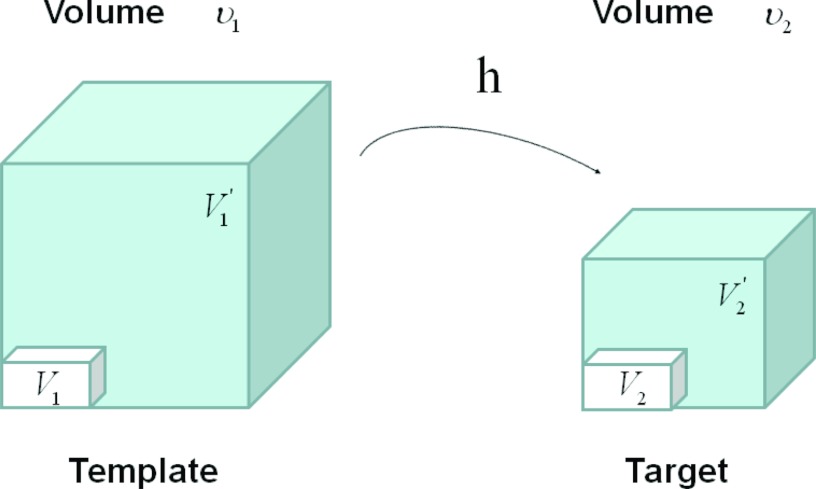
Figure 4 illustrates the assumption with no tissue volume change in SAI. In Fig. 4 as the region volume changes from ν₁ to ν₂, the tissue volume inside the cube remains the same (V₁ = V₂).

Figure 4.

Example of a given voxel under deformation h(x) from template image to target image, with the assumption of no tissue volume change. Notice the tissue volume V₁ = V₂ under this assumption. $V_1^{\prime }$ and $V_2^{\prime }$ are air volumes.

Difference of specific air volume change (DSA) and difference of tissue volume (DT):

Yin et al.²² have studied the tissue volume difference between max exhale and max inhale scans in human subjects, and the average difference is about 3.5%. Therefore, the assumption of SAI where tissue volume change is 0 may not be valid in estimating the regional specific air volume change. To investigate the relationship between the measurements of specific air volume changes and the tissue volume change, we can calculate the difference between Eqs. 15, 22 and define the DSA between SACJ and SAI, and the difference of DT as

$$\text{DSA}=|\text{SACJ}-\text{SAI}|,$$ (24)

$$\begin{array}{ccc}\hfill \text{DT}& =& |V_1\left(\mathbf{h}\left(\mathbf{x}\right)\right)-V_2\left(\mathbf{x}\right)|\hfill \end{array}$$ (25)

$$\begin{array}{ccc}& =& |{\nu }_1\left(\mathbf{h}\left(\mathbf{x}\right)\right)\beta \left(I_1\left(\mathbf{h}\left(\mathbf{x}\right)\right)\right)-{\nu }_2\left(\mathbf{x}\right)\beta \left(I_2\left(\mathbf{x}\right)\right)|\hfill \end{array}$$ (26)

$$\begin{array}{ccc}& =& |J\left(\mathbf{x}\right){\nu }_2\left(\mathbf{x}\right)\beta \left(I_1\left(\mathbf{h}\left(\mathbf{x}\right)\right)\right)-{\nu }_2\left(\mathbf{x}\right)\beta \left(I_2\left(\mathbf{x}\right)\right)|\hfill \end{array}$$ (27)

$$\begin{array}{ccc}& =& |{\nu }_2\left(\mathbf{x}\right)\frac{J\left(\mathbf{x}\right)(I_1\left(\mathbf{h}\left(\mathbf{x}\right)\right)-{\text{HU}}_{\text{air}})-(I_2\left(\mathbf{x}\right)-{\text{HU}}_{\text{air}})}{{\text{HU}}_{\text{tissue}}-{\text{HU}}_{\text{air}}}|\hfill \end{array}$$ (28)

Again, if we assume that air is −1000 HU and tissue is 0 HU, then the tissue volume difference is

$$\begin{array}{c}\hfill \text{DT}=|{\nu }_2\left(\mathbf{x}\right)\frac{J\left(\mathbf{x}\right)(I_1\left(\mathbf{h}\left(\mathbf{x}\right)\right)+1000)-(I_2\left(\mathbf{x}\right)+1000)}{1000}|\end{array}$$ (29)

Computational setup

Processing starts by identifying the lung regions in all images using the Pulmonary Workstation 2.0 (VIDA Diagnostics, Inc., Iowa City, IA). The Xe-CT estimate of sV is computed in the coordinates of the EE₀ using PASS (Ref. ¹⁸) at the original image size of 0.5 mm × 0.5 mm × 2.4 mm voxels. Overlapping 1 × 8 regions of interest (ROI) are defined in the lung region on each 2D slice. All images, including the EE, EI, EE₀ and their corresponding lung region masks or sV map, are then resampled to a voxel size of 1 mm × 1 mm × 1 mm. After preprocessing, EI is registered to EE using the TVP registration for measuring the regional ventilation from these two phases in a 4DCT scan. The resulting transformation is used to estimate the SAJ, SACJ, and SAI. Then EE₀ is registered to EE using TVP registration as well to map the sV to the same coordinate system as that of the SAJ, SACJ, and SAI. Due to the fact that the denominator of Eqs. 15, 22 may become zero, we eliminated from consideration any points that have the absolute value of the denominator become less than 0.001. For the TVP registration, the multiresolution strategy is used in the processing and it proceeds from low to high image resolution starting at one-eighth the spatial resolution and increases by a factor of 2 until the full resolution is reached. Meanwhile, a hierarchy of B-spline grid spaces from large to small is used. The finest B-spline grid space used in the experiments is 4 mm. The images and image grid space are refined alternatively.

Assessment of image registration accuracy

A semiautomatic landmark system is used for landmark selection and matching.³⁴ This system first uses an automatic landmark detection algorithm to find the landmarks in the EE image. The algorithm automatically detects “distinctive” points in the target image as the landmarks based on a distinctiveness value D(p). Around each point p, 45 points, q₁, …, q₄₅ are uniformly distributed on a spherical surface. A region of interest ROI(q_i) is compared with the corresponding region of interest ROI(p) around the original point, and then combined with its gradient value to calculate the distinctiveness value D(p).

The same system is then applied to guide the observer to match landmarks in the target image with corresponding landmarks in the template image. Each landmark-pair manually annotated by the observer is added to a thin-plate-spline to warp the template image. The system utilizes the warped image to estimate where the anatomic match will be located for a new landmark point presented to the observer, therefore the observer can start the matching from a system estimated location. Thus, as the warped image becomes more accurate by the new added landmarks, the task of the observer becomes easier.

For each animal, after 200 anatomic landmarks are identified in the EE image, the observer marks the locations of the voxels corresponding to the anatomic locations of the landmarks in the EI image. All the landmarks are verified by a second observer. A previous study³⁴ has reported the interobserver difference is below 2 mm using the same software. For each landmark, the actual landmark position is compared to the registration-derived estimate of landmark position and the error is calculated. With the evaluated accuracy of transformation from the lung image registration algorithm, the resulting regional ventilation measures estimated using the transformation can be then compared to Xe-CT estimated ventilation.

Compare registration regional ventilation measures to Xe-CT estimated ventilation

In our previous work,^{4, 6} regional lung expansion, as estimated from the Jacobian of the image registration transformations, was compared with Xe-CT based sV. The analysis was conducted by evaluating Jacobian value between a pair of lung volumes from static (multiple airway pressures) and dynamic image datasets, and comparing the Jacobian along the y (ventral-dorsal) axis. While the correlation between the Jacobian value and sV reflect the fact that regional expansion estimated from image registration can be used as an index as regional lung function, the spatial resolution of the analysis method employed were likely not sufficient to distinguish the differences between regional ventilation measures as we have described in Sec. 2D. Therefore, to locally compare the regional ventilation measures, the corresponding region of Xe-CT image EE₀ in the EE is divided into approximately 100 nonoverlapping cubes with size of 20 mm × 20 mm × 20 mm. We compare the average regional ventilation measures (SAJ, SACJ, and SAI) to the corresponding average sV measurement from Xe-CT images within each cube. The correlation coefficients between any two estimates (SAJ-sV, SACJ-sV or SAI-sV) are calculated by linear regression. To compare two correlation coefficients, the Fisher Z-transform of the r values is used and the level of significance is determined.³⁵ The relationship between the specific air volume change and difference of tissue volume is also studied in four animals by linear regression analysis.

RESULTS

Registration accuracy

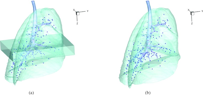
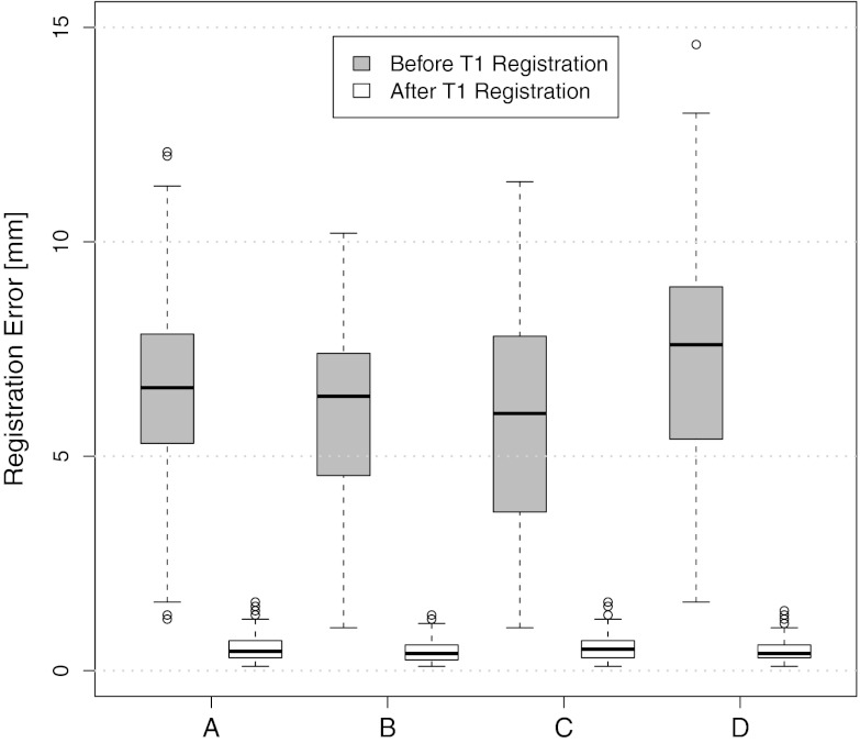
For each animal, approximately 200 automatically identified landmarks within the lungs are used to compute registration accuracy. The landmarks are widely distributed throughout the lung regions. Figure 5 shows an example of the distribution of the landmarks in animal D for both the EE and EI images. The coordinate of each landmark location is recorded for each image dataset before and after registration for all four animals. Figure 6 shows the landmark distance before and after registration for four animals. The gray boxes show the magnitude of respiratory motion during the tidal breathing. For all four animals, before registration, the average landmark distance is 6.6 mm with a minimum distance of 1.0 mm, maximum distance of 14.6 mm, and standard deviation of 2.42 mm. After registration, the average landmark distance is 0.4 mm with a minimum distance of 0.1 mm, a maximum distance of 1.6 mm, and a standard deviation 0.29 mm. The trends for all animals are consistent and the results demonstrate that the registrations produced good anatomic correspondences. All registrations were examined and it was confirmed that all Jacobian values had positive values.

Figure 5.

3D view of the landmarks in (a) EE with EE₀ and (b) EI. The dark region below the carina in (a) is the EE₀ and the spheres are the automatically defined landmarks.

Figure 6.

Landmarks distances of the registration pair EI to EE for all four animals. Boxplot lower extreme is first quartile, boxplot upper extreme is third quartile. Median is shown with solid horizontal line. Whiskers show either the minimum (maximum) value or extend 1.5 times the first to third quartile range beyond the lower (upper) extreme of the box, whichever is smaller (larger). Outliers are marked with circles.

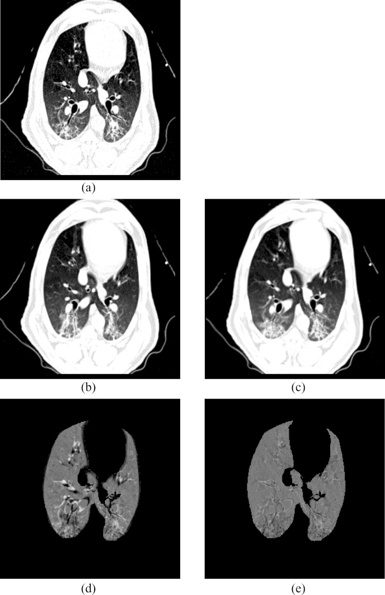
Figure 5a shows the location of the EE₀ (Xe-CT) slab overlaid on the EE image. Figure 7 shows an example of the image registration result from the EE₀ image to the EE image. The first row shows the misalignment between the images before image registration. Though the images were acquired without moving the animal between the scans, there is still nonrigid deformation between scans as shown in Fig. 7d, as the black and white regions represent the large intensity difference between Figs. 7a, 7b. In addition, the slice thicknesses were quite different which causes partial volume artifacts. After image registration, the EE₀ image is aligned to the EE image, and the resulting difference image [shown in Fig. 7e] is near zero. The transformation from the EE₀ to the EE image allows us to map the Xe-CT sV into the coordinate system of EE image. Note that since the regions outside the lung are not included in the registration process, the mediastinum and other body tissues are not aligned. Also note that the dorsal region of the lung shows a intensity difference after registration. This is due mainly to the gradual progression of atelectasis and tissue edema during the course of the experiment.

Figure 7.

Visualization of the result of the transformation that maps the Xe-CT estimated ventilation sV to the EE coordinate system: (a) EE, (b) EE₀, (c) deformed EE₀ after registration, (d) intensity difference between EE and EE₀ before registration, (e) intensity difference between EE and EE₀ after registration.

Registration estimated ventilation compared to Xe-CT estimated ventilation

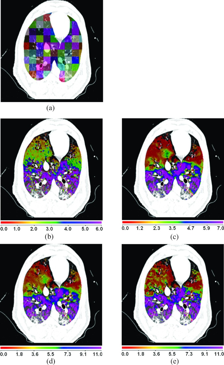
Figure 8a shows a comparison between the registration-derived indices of ventilation and the Xe-CT estimated sV in cube-shaped regions of interest for animal D. The corresponding Xe-CT regions in the EE are divided into about 100 cubes. Figure 8b is the Xe-CT estimate of sV. Figures 8c, 8d, 8e are the corresponding registration ventilation measures SAJ, SACJ, and SAI. The regions with edema are excluded from the comparison. Figures 8b, 8c, 8d all show noticeable similar gradient in the ventral-dorsal direction. Notice that the color scales are different in each map and are set based on the range of values from the appropriate plot in Fig. 9.

Figure 8.

Comparison of the regional ventilation measures for animal D. (a) EE with color coded cubes showing the sample region. (b)–(e) Color map of the sV, SAJ, SACJ, and SAI. Note that the color scales are different for (b)–(e), and are set based on the range of values from the appropriate plot in Fig. 9. The results were similar for the other three animals.

Figure 9.

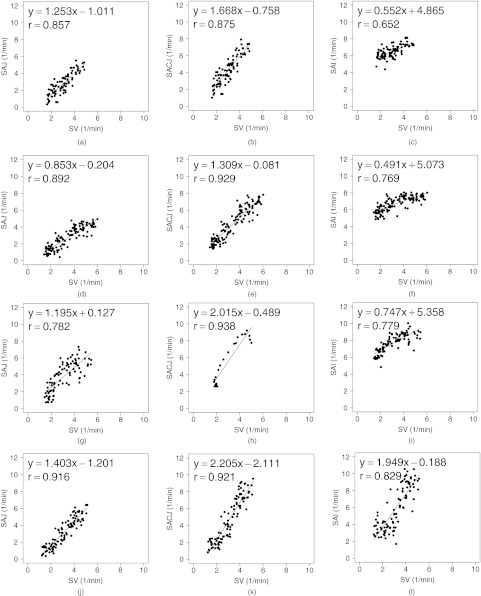
Small cube ROIs with size 20 mm × 20 mm × 20 mm results for registration estimated ventilation measures compared to the Xe-CT estimated ventilation sV in scatter plot with linear regression in four animals. The first column is the SAJ vs sV. The second column is the SACJ vs sV. The third column is the SAI vs sV.

Figure 9 shows scatter plots comparing the registration ventilation measures and the Xe-CT ventilation sV in all four animals. The SACJ column shows the strongest correlation with the sV (average r² = 0.82). The SAJ, which is directly related to Jacobian as SAJ = J − 1, also shows good correlation with the sV (average r² = 0.75). The intensity-based measure SAI shows the lowest correlation with the sV (average r² = 0.58).

Table 1 shows the results of comparing the r values from SACJ vs sV and SAI vs sV. All four animals show that the correlation coefficient from SACJ vs sV is significantly stronger than it from SAI vs sV. Similarly, Table 2 shows the results of comparing the r values from SAJ vs sV and SAI vs sV. The registration ventilation measure SAJ also shows a significantly stronger correlation with sV than SAI. Comparing the r values from SACJ vs sV and SAJ vs sV as in Table 3, only animal B and C show that the SACJ has significantly stronger correlation with sV than SAJ.

Table 1.

Comparison of ventilation measures between SACJ and SAI in small cube ROIs with size 20 mm × 20 mm × 20 mm.

	Correlation	Correlation with sV	Number of	SACJ vs SAI
Animal	pair	(r value)	samples	p value
A	SACJ vs sV	0.88	83	p < = 0.0001
	SAI vs sV	0.65
B	SACJ vs sV	0.93	119	p < = 1.18e−6
	SAI vs sV	0.77
C	SACJ vs sV	0.89	86	p < = 0.0075
	SAI vs sV	0.78
D	SACJ vs sV	0.92	110	p < = 0.0017
	SAI vs sV	0.83

Table 2.

Comparison of ventilation measures between SAJ and SAI in small cube ROIs with size 20 mm × 20 mm × 20 mm.

	Correlation	Correlation with sV	Number of	SAJ vs SAI
Animal	pair	(r value)	samples	p value
A	SAJ vs sV	0.86	83	p < = 0.0005
	SAI vs sV	0.65
B	SAJ vs sV	0.89	119	p < = 0.002
	SAI vs sV	0.77
C	SAJ vs sV	0.78	86	p < = 0.5
	SAI vs sV	0.78
D	SAJ vs sV	0.92	110	p < = 0.0017
	SAI vs sV	0.83

Table 3.

Comparison of ventilation measures between SACJ and SAJ in small cube ROIs with size 20 mm × 20 mm × 20 mm.

	Correlation	Correlation with sV	Number of	SACJ vs SAJ
Animal	pair	(r value)	samples	p value
A	SACJ vs sV	0.88	83	p < = 0.302
	SAJ vs sV	0.86
B	SACJ vs sV	0.93	119	p < = 0.035
	SAJ vs sV	0.89
C	SACJ vs sV	0.89	86	p < = 0.007
	SAJ vs sV	0.78
D	SACJ vs sV	0.92	110	p < = 0.5
	SAJ vs sV	0.92

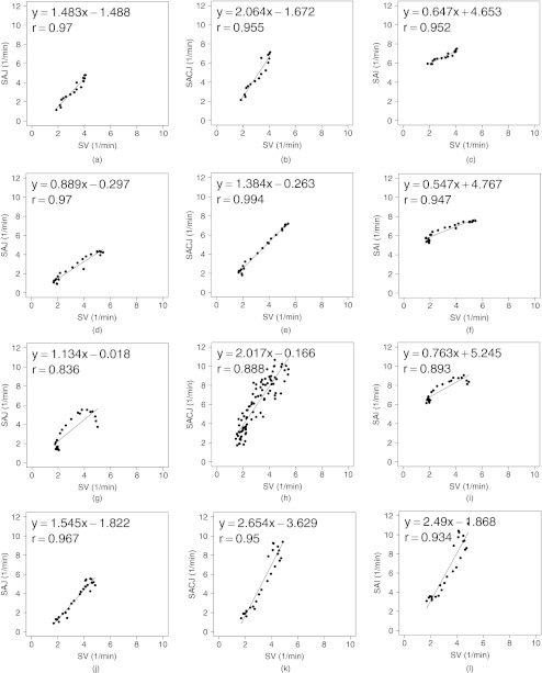
To analyze the effect of the size of the region of interest, the corresponding region of Xe-CT image EE₀ in the EE is divided into about 30 slabs along the ventral-dorsal direction with size of 150 mm × 8 mm × 40 mm as similarly in our previous work.^{4, 6} Figure 10 shows the scatter plots between the registration ventilation measures and the Xe-CT ventilation sV similar as Fig. 10 but in larger ROIs. The SACJ column shows the strongest correlation with the sV (average r² = 0.92). Both the SAJ and SAI show good correlation with sV as well (average r² = 0.88 and r² = 0.87). However, though the average r² value still show the SACJ has the highest correlation with Xe-CT based sV, Tables 4, 5 show that with larger averaging region as defined slabs, there is no significant difference between the correlation coefficients from SACJ vs sV and SAI vs sV, between SAJ vs sV and SAI vs sV, or SACJ vs sV and SAJ vs sV as in Table 6.

Figure 10.

Large slab ROIs with size 150 mm × 8 mm × 40 mm results for registration estimated ventilation measures compared to the Xe-CT estimated ventilation sV in scatter plot with linear regression in four animals. The first column is the SAJ vs sV. The second column is the SACJ vs sV. The third column is the SAI vs sV.

Table 4.

Comparison of ventilation measures between SACJ and SAI in large slab ROIs with size 150 mm × 8 mm × 40 mm.

	Correlation	Correlation with sV	Number of	SACJ vs SAI
Animal	pair	(r value)	samples	p value
A	SACJ vs sV	0.95	17	p < = 0.5
	SAI vs sV	0.95
B	SACJ vs sV	0.99	23	p < = 0.005
	SAI vs sV	0.95
C	SACJ vs sV	0.94	23	p < = 0.15
	SAI vs sV	0.89
D	SACJ vs sV	0.95	25	p < = 0.28
	SAI vs sV	0.93

Table 5.

Comparison of ventilation measures between SAJ and SAI in large slab ROIs with size 150 mm × 8 mm × 40 mm.

	Correlation	Correlation with sV	Number of	SAJ vs SAI
Animal	pair	(r value)	samples	p value
A	SAJ vs sV	0.95	17	p < = 0.5
	SAI vs sV	0.95
B	SAJ vs sV	0.99	23	p < = 0.005
	SAI vs sV	0.95
C	SAJ vs sV	0.94	23	p < = 0.16
	SAI vs sV	0.89
D	SAJ vs sV	0.95	25	p < = 0.28
	SAI vs sV	0.93

Table 6.

Comparison of ventilation measures between SACJ and SAJ in large slab ROIs with size 150 mm × 8 mm × 40 mm.

	Correlation	Correlation with sV	Number of	SACJ vs SAI
Animal	pair	(r value)	samples	p value
A	SACJ vs sV	0.95	17	p < = 0.5
	SAJ vs sV	0.95
B	SACJ vs sV	0.99	23	p < = 0.5
	SAJ vs sV	0.99
C	SACJ vs sV	0.94	23	p < = 0.5
	SAJ vs sV	0.94
D	SACJ vs sV	0.95	25	p < = 0.5
	SAJ vs sV	0.95

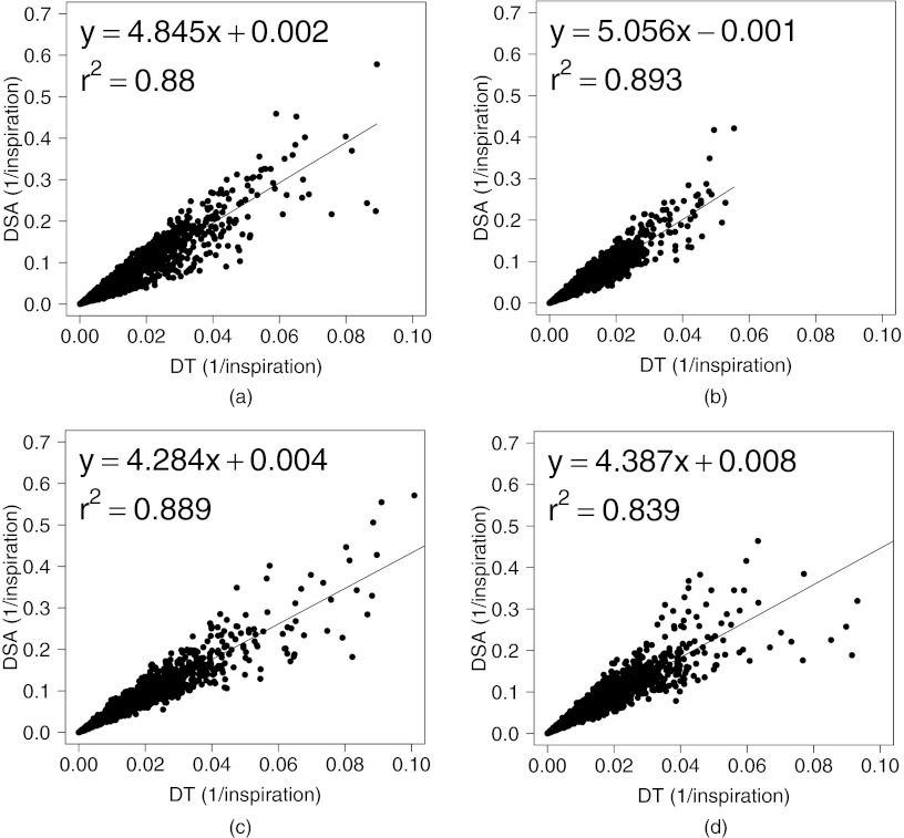
Figure 11 shows the scatter plots between DSA (the absolute difference of the value between the SACJ and SAI) and the DT (the absolute difference of the tissue volume) with linear regression in all four animals (average r² = 0.86). From Eqs. 15, 22, we know that the SAI measurement assumes no tissue volume change in a given region being registered, which may not be valid assumption in all lung regions. Figure 11 shows that as the tissue volume change increases, the difference between the measures of regional ventilation from SACJ and SAI increases linearly in all four animals. It indicates that the lower correlation of SAI with sV compared with SACJ with sV may be caused by the tissue volume change between two volumes.

Figure 11.

Linear regression analysis between DSA and DT. (a)–(d) DSA (the absolute difference of the value between the SACJ and SAI) compared to DT (the absolute difference of the tissue volume) in animals A, B, C, and D.

SUMMARY AND CONCLUSIONS

We described three measures to estimate regional lung tissue ventilation from tissue volume and vesselness preserving image registration of CT images. These measures have been compared with each other, and compared to Xe-CT estimates of specific ventilation. We examined the assumption of constant tissue volume between registered lung regions, and demonstrated that the difference between two of the registration derived measures (SACJ and SAI) may be explained by differences in tissue volume between the lung regions being compared with registration.

The tissue volume and vesselness preserving nonlinear registration algorithm was used to match the EI image to the EE image to produce the registration deformation field and estimates of regional ventilation. It was used to register the EE₀ image to the EE image for comparing the three ventilation measures to the Xe-CT based sV. About 200 anatomical landmarks were identified and annotated in each dataset to evaluate registration accuracy. The average landmark error is on the order of 1 mm after registration.

The ventilation measures SAJ, SACJ, and SAI were derived using a simple model of a lung region, containing a mixture of air and tissue, which deforms during inspiration or exhalation. The SAJ measure, which is a linear function of the Jacobian of the registration displacement field, measures regional ventilation based on the assumption that the lung region contains only air (i.e., no tissue volume). The SACJ is the most general form of the three measures and is based on model where both the air and tissue volumes can change during inspiration and exhalation. Finally, the SAI measure is computed based on intensity change alone, and assumes that the region may have a tissue volume that is nonzero, but this volume does not change during inspiration and exhalation. Thus, the SAJ measure relies solely on the volume change information computed from the Jacobian of the deformation field and the SAI measure relies solely on the change in region intensity as measured by the CT. The SACJ measure uses a more complete model of local ventilation, and combines the geometric information from the Jacobian with the density information calculated from the change in region intensity.

The three registration-based ventilation measures and the Xe-CT sV measurement were averaged and compared in cubic-shaped regions of interest. In 20 mm × 20 mm × 20 mm ROIs, the SACJ shows significantly higher correlation with Xe-CT sV than the SAI in all four animals. By studying the difference between the SACJ and SAI measures and the tissue volume difference estimated by the CT intensity change, we showed that the difference between SACJ and SAI may be explained by the constant tissue volume assumption implicit in the SAI model 19. From Fig. 11, we see that the difference between the SACJ and SAI measures is approximately linearly related to the estimated tissue volume change. Tables 1, 2 show that the both the SACJ and SAJ have significantly better correlation with sV than the SAI. This is consistent with the findings by Kabus et al.³⁶ who showed that the Jacobian-based measure of ventilation has less error than the intensity-based ventilation measure, using the segmented total lung volume as a global comparison. Though all the regional ventilation measures and Xe-CT based sV from the linear regression analysis in Fig. 10 show high correlations, Tables 4, 5 show that there is no significant difference in the correlation with sV between the Jacobian-based measures and intensity-based measure. This result indicates that the validation methods using global comparison such as segmented total volume may not be able to distinguish the Jacobian-based measure and the intensity-based measure.

The comparison of the ventilation measures was limited to the resolution of 20 mm × 20 mm × ROIs. As the size of the ROIs decreases, the correlation between the ventilation measures with Xe-CT based sV decreases. This may be due to the underlying noise of the Xe-CT measurement of ventilation or the decreased sensitivity of registration based measure to local ventilation heterogeneity which is relative to the case. Additional Xe-CT image analysis work including using multicompartment models, thinner slice, and inter-phase registration to improve sV measurement are required to reduce the noise in Xe-CT based sV measurement.

To compare with the intensity-based ventilation measure used in previous work in Simon,³² Guerrero et al.,¹¹ and Fuld et al.,³³ we followed the assumption that HU_air is −1000 HU and HU_tissue is 0 HU (equaling water²⁵) in this work. The ventilation measures were calculated under the assumption that HU_air is −1000 HU and HU_tissue is 55 HU, which are the values used by Yin et al.²² Our analysis shows that the correlation coefficients between any two estimates (SAJ-sV, SACJ-sV or SAI-sV) change less than 1% with two different HU_tissue values. However, it would be important to have sensitivity analysis in the future to compare different ventilation measures against intensity changes.

The image registration algorithm used to find the transformation from EI to EE for measurement of regional ventilation produces accurate registrations by minimizing the tissue volume and vesselness measure difference between the template image and the target image. It would be interesting to compare different image registration algorithms and their effects on the registration based ventilation measures. For example, if two registration algorithms achieve the similar landmark accuracy, the one does not preserve tissue volume change may show even larger difference in the SACJ and SAI measures than the results using TVP as described above.

In conclusion, with the same deformation field by the same image registration algorithm, a significant difference between the Jacobian/-corrected Jacobian-based ventilation measures and the intensity-based ventilation measure is found in a regional level using Xe-CT based ventilation measure sV. The ventilation measure by corrected Jacobian SACJ gives best correlation with Xe-CT based sV and the correlation is significantly higher than from the ventilation by intensity SAI indicating the ventilation measure by corrected Jacobian SACJ may be a better measure of regional lung ventilation from image registration of 4DCT images.

References

- Keall P. J., Kini V. R., Vedam S. S., and Mohan R., “Potential radiotherapy improvements with respiratory gating,” Australas. Phys. Eng. Sci. Med. 25(1), 1–6 (2002). 10.1007/BF03178368 [DOI] [PubMed] [Google Scholar]
- Low D. A., Nystrom M., Kalinin E., Parikh P., Dempsey J. F., Bradley J. D., Mutic S., Wahab S. H., Islam T., Christensen G., Politte D. G., and Whiting B. R., “A method for the reconstruction of four-dimensional synchronized CT scans acquired during free breathing,” Med. Phys. 30(6), 1254–1263 (2003). 10.1118/1.1576230 [DOI] [PubMed] [Google Scholar]
- Pan T., “Comparison of helical and cine acquisitions for 4D-CT imaging with multislice CT,” Med. Phys. 32(2), 627–634 (2005). 10.1118/1.1855013 [DOI] [PubMed] [Google Scholar]
- Reinhardt J. M., Ding K., Cao K., Christensen G. E., Hoffman E. A., and Bodas S. V., “Registration-based estimates of local lung tissue expansion compared to xenon CT measures of specific ventilation,” Med. Image Anal. 12(6), 752–763 (2008), special issue on information processing in medical imaging 2007. 10.1016/j.media.2008.03.007 [DOI] [PMC free article] [PubMed] [Google Scholar]
- Ding K., Cao K., Christensen G. E., Raghavan M. L., Hoffman E. A., and Reinhardt J. M., “Registration-based lung tissue mechanics assessment during tidal breathing,” in First International Workshop on Pulmonary Image Analysis, edited by Brown M., de Bruijne M., van Ginneken B., Kiraly A., Kuhnigk J.-M., Lorenz C., Mori K., and Reinhardt J. M. (Lulu, New York, 2008), p. 63. [Google Scholar]
- Ding K., Cao K., Christensen G. E., Hoffman E. A., and Reinhardt J. M., “Registration-based regional lung mechanical analysis: Retrospectively reconstructed dynamic imaging versus static breath-hold image acquisition, Medical Imaging 2009: Biomedical Applications in Molecular, Structural, and Functional Imaging,” in Proceedings of SPIE Conference Medical Imaging, edited by Hu X. P. and Clough A. V. (SPIE, Lake Buena Vista, FL, 2009), Vol. 7262(1), p. 72620D. 10.1117/12.813694 [DOI]
- Ding K., Yin Y., Cao K., Christensen G. E., Lin C.-L., Hoffman E. A., and Reinhardt J. M., “Evaluation of lobar biomechanics during respiration using image registration,” in Proceedings of International Conference on Medical Image Computing and Computer-Assisted Intervention 2009 (Springer, London, UK, 2009), Vol. 5761, pp. 739–746. 10.1007/978-3-642-04268-3_91 [DOI] [PMC free article] [PubMed]
- Yaremko B. P., Guerrero T. M., Noyola-Martinez J., Guerra R., Lege D. G., Nguyen L. T., Balter P. A., Cox J. D., and Komaki R., “Reduction of normal lung irradiation in locally advanced non-small-cell lung cancer patients, using ventilation images for functional avoidance,” Int. J. Radiat. Oncol., Biol., Phys. 68(2), 562–571 (2007). 10.1016/j.ijrobp.2007.01.044 [DOI] [PMC free article] [PubMed] [Google Scholar]
- Yamamoto T., Kabus S., von Berg J., Lorenz C., and Keall P. J., “Impact of four-dimensional computed tomography pulmonary ventilation imaging-based functional avoidance for lung cancer radiotherapy,” Int. J. Radiat., Oncol., Biol., Phys. 2, 1–10 (2010). 10.1016/j.ijrobp.2010.02.008 [DOI] [PubMed] [Google Scholar]
- Ding K., Bayouth J. E., Buatti J. M., Christensen G. E., and Reinhardt J. M., “4DCT-based measurement of changes in pulmonary function following a course of radiation therapy,” Med. Phys. 37(3), 1261–1272 (2010). 10.1118/1.3312210 [DOI] [PMC free article] [PubMed] [Google Scholar]
- Guerrero T., Sanders K., Noyola-Martinez J., Castillo E., Zhang Y., Tapia R., Guerra R., Borghero Y., and Komaki R., “Quantification of regional ventilation from treatment planning CT,” Int. J. Radiat. Oncol., Biol., Phys. 62(3), 630–634 (2005). 10.1016/j.ijrobp.2005.03.023 [DOI] [PubMed] [Google Scholar]
- Guerrero T., Sanders K., Castillo E., Zhang Y., Bidaut L., and Komaki T. P. R., “Dynamic ventilation imaging from four-dimensional computed tomography,” Phys. Med. Biol. 51(4), 777–791 (2006). 10.1088/0031-9155/51/4/002 [DOI] [PubMed] [Google Scholar]
- Christensen G. E., Song J. H., Lu W., Naqa I. E., and Low D. A., “Tracking lung tissue motion and expansion/compression with inverse consistent image registration and spirometry,” Med. Phys. 34(6), 2155–2165 (2007). 10.1118/1.2731029 [DOI] [PubMed] [Google Scholar]
- Castillo R., Castillo E., Martinez J., and Guerrero T., “Ventilation from four-dimensional computed tomography: Density versus jacobian methods,” Phys. Med. Biol. 55(16), 4661–4685 (2010). 10.1088/0031-9155/55/16/004 [DOI] [PubMed] [Google Scholar]
- Marcucci C., Nyhan D., and Simon B. A., “Distribution of pulmonary ventilation using Xe-enhanced computed tomography in prone and supine dogs,” J. Appl. Physiol. 90(2), 421–430 (2001). 10.1063/1.1376412 [DOI] [PubMed] [Google Scholar]
- Tajik J. K., Chon D., Won C.-H., Tran B. Q., and Hoffman E. A., “Subsecond multisection CT of regional pulmonary ventilation,” Acad. Radiol. 9, 130–146 (2002). 10.1016/S1076-6332(03)80163-0 [DOI] [PubMed] [Google Scholar]
- Chon D., Simon B. A., Beck K. C., Shikata H., Saba O. I., Won C., and Hoffman E. A., “Differences in regional wash-in and wash-out time constants for xenon-CT ventilation studies,” Respir. Physiol. Neurbiol. 148(1-2), 65–83 (2005). 10.1016/j.resp.2005.06.003 [DOI] [PubMed] [Google Scholar]
- Guo J., Fuld M. K., Alford S. K., Reinhardt J. M., and Hoffman E. A., “Pulmonary Analysis Software Suite 9.0: Integrating quantitative measures of function with structural analyses,” in First International Workshop on Pulmonary Image Analysis (Lulu, New York, 2008), pp. 283–292. [Google Scholar]
- Cao K., Ding K., Christensen G. E., and Reinhardt J. M., “Tissue volume and vesselness measure preserving nonrigid registration of lung CT images,” in Proceedings of SPIE Conference Medical Imaging, edited by Dawant B. M. and Haynor D. R. (SPIE, San Diego, CA, 2010), Vol. 7623(1), p. 762309. 10.1117/12.844541 [DOI]
- Cao K., Ding K., Christensen G. E., Raghavan M. L., Amelon R. E., and Reinhardt J. M., “Unifying vascular information in intensity-based nonrigid lung CT registration,” in Biomedical Image Registration, edited by Fischer B., Dawant B., and Lorenz C. (Springer, Lübeck, 2010), pp. 1–12. [Google Scholar]
- Yin Y., Hoffman E. A., and Lin C.-L., “Local tissue-weight-based nonrigid registration of lung images with application to regional ventilation, Medical Imaging 2009: Biomedical Applications in Molecular, Structural, and Functional Imaging,” in Proceedings of SPIE Conference Medical Imaging, edited by Hu X. P. and Clough A. V. (SPIE, Lake Buena Vista, FL, 2009), Vol. 7262(1), p. 72620C. 10.1117/12.811715 [DOI]
- Yin Y., Hoffman E. A., and Lin C.-L., “Mass preserving nonrigid registration of CT lung images using cubic B-spline,” Med. Phys. 36(9), 4213–4222 (2009). 10.1118/1.3193526 [DOI] [PMC free article] [PubMed] [Google Scholar]
- Cao K., Christensen G. E., Ding K., and Reinhardt J. M., “Intensity-and-landmark-driven, inverse consistent, B-spline registration and analysis for lung imagery,” in Second International Workshop on Pulmonary Image Analysis, edited by Brown M., de Bruijne M., van Ginneken B., Kiraly A., Kuhnigk J.-M., Lorenz C., McClelland J. R., Mori K., Reeves A., and Reinhardt J. M. (CreateSpace, London, UK, 2009), p. 137. [Google Scholar]
- Yin Y., Choi J., Hoffman E. A., Tawhai M. H., and Lin C.-L., “Simulation of pulmonary air flow with a subject-specific boundary condition,” J. Biomech. 43(11), 2159–2163 (2010). 10.1016/j.jbiomech.2010.03.048 [DOI] [PMC free article] [PubMed] [Google Scholar]
- Hoffman E. A. and Ritman E. L., “Effect of body orientation on regional lung expansion in dog and sloth,” J. Appl. Physiol. 59(2), 481–491 (1985). [DOI] [PubMed] [Google Scholar]
- Frangi A. F., Niessen W. J., Vincken K. L., and Viergever M. A., “Multiscale vessel enhancement filtering,” in Proceedings of International Conference on Medical Image Computing and Computer-Assisted Intervention 1998 (Springer, Cambridge, MA, 1998), Vol. 1496, pp. 130–137.
- Shikata H., Hoffman E. A., and Sonka M., “Automated segmentation of pulmonary vascular tree from 3D CT images, Medical Imaging 2004: Physiology, Function, and Structure from Medical Images,” in Proceedings of SPIE Conference Medical Imaging, edited by Amini A. A. and Manduca A. (SPIE, San Diego, CA, 2004), Vol. 5369(1), pp. 107–116. 10.1117/12.537032 [DOI]
- Shikata H., McLennan G., Hoffman E. A., and Sonka M., “Segmentation of pulmonary vascular trees from thoracic 3D CT images,” Int. J. Biomed. Imaging 2009(1), 36240 (2009). 10.1155/2009/636240 [DOI] [PMC free article] [PubMed] [Google Scholar]
- Joshi V., Reinhardt J. M., and Abramoff M. D., “Automated measurement of retinal blood vessel tortuosity,” in Proceedings of SPIE Conference Medical Imaging, edited by Karssemeijer N. and Summers R. M. (SPIE, San Diego, CA, 2010), Vol. 7624, p. 76243. 10.1117/12.844641 [DOI]
- Byrd R. H., Lu P., Nocedal J., and Zhu C., “A limited memory algorithm for bound constrained optimization,” SIAM J. Sci. Comput. (USA) 16(5), 1190–1208 (1995). 10.1137/0916069 [DOI] [Google Scholar]
- Choi Y. and Lee S., “Injectivity conditions of 2D and 3D uniform cubic b-spline functions,” Graphical Models 62(6), 411–427 (2000). 10.1006/gmod.2000.0531 [DOI] [Google Scholar]
- Simon B. A., “Non-invasive imaging of regional lung function using x-ray computed tomography,” J. Clin. Monit Comput. 16(5), 433–442 (2000). 10.1023/A:1011444826908 [DOI] [PubMed] [Google Scholar]
- Fuld M. K., Easley R. B., Saba O. I., Chon D., Reinhardt J. M., Hoffman E. A., and Simon B. A., “CT-measured regional specific volume change reflects regional ventilation in supine sheep,” J. Appl. Physiol. 104(4), 1177–1184 (2008). 10.1152/japplphysiol.00212.2007 [DOI] [PubMed] [Google Scholar]
- Murphy K., van Ginneken B., Pluim J., Klein S., and Staring M., “Semi-automatic reference standard construction for quantitative evaluation of lung CT registration,” in Proceedings of International Conference on Medical Image Computing and Computer-Assisted Intervention 2008 (Springer, New York, NY, 2008), Vol. 5242, pp. 1006–1013. 10.1007/978-3-540-85990-1_121 [DOI] [PubMed]
- Probability and Statistics, edited by Papoulis A. (Prentice-Hall, Englewood Cliffs, NJ, 1990). [Google Scholar]
- Kabus S., von Berg J., Yamamoto T., Opfer R., and Keall P. J., “Lung ventilation estimation based on 4D-CT imaging,” in First International Workshop on Pulmonary Image Analysis (Lulu, New York, 2008), pp. 73–81.