A Bayesian model of shape and appearance for subcortical brain segmentation

Abstract

Automatic segmentation of subcortical structures in human brain MR images is an important but difficult task due to poor and variable intensity contrast. Clear, well-defined intensity features are absent in many places along typical structure boundaries and so extra information is required to achieve successful segmentation. A method is proposed here that uses manually labelled image data to provide anatomical training information. It utilises the principles of the Active Shape and Appearance Models but places them within a Bayesian framework, allowing probabilistic relationships between shape and intensity to be fully exploited. The model is trained for 15 different subcortical structures using 336 manually-labelled T1-weighted MR images. Using the Bayesian approach, conditional probabilities can be calculated easily and efficiently, avoiding technical problems of ill-conditioned covariance matrices, even with weak priors, and eliminating the need for fitting extra empirical scaling parameters, as is required in standard Active Appearance Models. Furthermore, differences in boundary vertex locations provide a direct, purely local measure of geometric change in structure between groups that, unlike voxel-based morphometry, is not dependent on tissue classification methods or arbitrary smoothing. In this paper the fully-automated segmentation method is presented and assessed both quantitatively, using Leave-One-Out testing on the 336 training images, and qualitatively, using an independent clinical dataset involving Alzheimer’s disease. Median Dice overlaps between 0.7 and 0.9 are obtained with this method, which is comparable or better than other automated methods. An implementation of this method, called FIRST, is currently distributed with the freely-available FSL package.

Introduction

It is important that medical image segmentation methods are accurate and robust in order to sensitively study both normal and pathological brains. Achieving this in the subcortical areas of the brain, given the typical low contrast-to-noise, is a great challenge for automated methods. When trained human specialists perform manual segmentations they draw on prior knowledge of shape, image intensities and shape-to-shape relationships. We present here a formulation of a computationally efficient shape and appearance model based on a Bayesian framework that incorporates both intra-and inter-structure variability information, while also taking account of the limited size of the training set with respect to the dimensionality of the data. The method is capable of performing segmentations of individual or multiple subcortical structures as well as analysing differences in shape between different groups, showing the location of changes in these structures, rather than just changes in the overall volume.

The Active Shape Model (ASM) is an automated segmentation method that has been widely used in the field of machine vision and medical image segmentation over the past decade (Cootes et al., 1995). Standard ASMs model the distribution of corresponding anatomical points (vertices/control points) and then parameterize the mean shape and most likely variations of this shape across a training set. Images are segmented using the model built from the training data, which specifies the range of likely shapes. In the original formulation, if the dimensionality of the shape representation exceeds the size of the training data then the only permissible shapes are linear combinations of the original training data, although some methods for generalising this have been presented in the literature (Heimann and Meinzer, 2009).

Intensity models are also useful in segmentation, and the Active Appearance Model (AAM) is an extension of the ASM framework that incorporates such intensity information (Cootes et al., 1998). As with the standard shape model, the intensity distribution is modelled as a multivariate Gaussian and is parameterized by its mean and eigenvectors (modes of variation). The AAM relates the shape and intensity models to each other with a weighting matrix estimated from the training set. Fitting shapes to new images is done by minimising the squared difference between the predicted intensities, given a shape deformation, and the observed image intensities. Again, many modifications of this basic formulation have also been proposed (Heimann and Meinzer, 2009).

In addition to the ASM and AAM methods there are many other approaches taken by fully-automated segmentation methods for subcortical structures. Some of these methods are specific to particular structures (e.g. hippocampus), others can be applied to general structures and still others can be applied to multiple structures simultaneously. The approaches can be surface-based, volumetric-based or both, and utilise methods such as: region competition (Chupin et al., 2007, 2009); homotopic region deformation (Lehéricy et al., 2009); level-sets within a Bayesian framework (Cremers et al., 2006) or with local distribution models (Yan et al., 2004); 4D shape priors (Kohlberger et al., 2006); probabilistic boosting trees (Wels et al., 2008); label, or classifier, fusion (Heckemann et al., 2006); label fusion with templates (Collins and Pruessner, 2010); label fusion with graph cuts (Wolz et al., 2010); wavelets with ASM (Davatzikos et al., 2003); multivariate discriminant methods (Arzhaeva et al., 2006); medial representations or deformable M-reps (Levy et al., 2007; Styner et al., 2003); probabilistic boosting trees (Tu et al., 2008); large diffeomorphic mapping (Lee et al., 2009b); and non-linear registration combined with AAM (Babalola et al., 2007).

The most common volumetric-based approaches to segmentation are based on non-linear warping of an atlas, or atlases, to new data (Collins and Evans, 1997; Fischl et al., 2002; Pohl et al., 2006). Traditionally, a single average atlas has been used to define the structure segmentations (as in (Collins and Evans, 1997; Gouttard et al., 2007)) whereas recent methods (Gousias et al., 2008; Heckemann et al., 2006) propagate information from multiple atlases and fuse the results. Additional information such as voxel-wise intensity and shape priors can also be utilised (Fischl et al., 2002; Khan et al., 2008). When using a single atlas, only a very limited amount of information on shape variation from the training data can be retained. In place of this shape information, registration methods define the likelihood of a given shape via the space of allowable transformations and regularisation-based penalization applied to them. This potentially biases the segmented shapes to favour smooth variations about the average template. Alternatively, methods that use multiple atlases or additional voxel-wise shape priors are able to retain more variational information from the training data.

Surface-based methods, on the other hand, tend to explicitly use learned shape variation as a prior in the segmentation (Colliot et al., 2006; Pitiot et al., 2004; Tsai et al., 2004). In brain image segmentation various ways of representing shapes and relationships have been proposed, including fuzzy models (Colliot et al., 2006), level-sets (Tsai et al., 2004), and simplex meshes (Pitiot et al., 2004). In addition, an array of different approaches has been taken to couple the intensities in the image to the shape, usually in the form of energies and/or forces, which often require arbitrary weighting parameters to be set.

Our approach takes the deformable-model-based AAM and poses it in a Bayesian framework. This framework is advantageous as it naturally allows probability relationships between shapes of different structures and between shape and intensity to be utilised and investigated, while also accounting for the limited amount of training data in a natural way. It is still based on using a deformable model that restricts the topology (unlike level-sets or voxel-wise priors), which is advantageous since the brain structures we are interested in have a fixed topology, as confirmed by our training data. Another benefit of the deformable model is that point correspondence between structures is maintained. This allows vertex-wise structural changes to be detected between groups of subjects, facilitating investigations of normal and pathological variations in the brain. Moreover, this type of analysis is purely local, based directly on the geometry/location of the structure boundary and is not dependent on tissue-type classification or smoothing extents, unlike voxel-based morphometry methods.

One difficulty of working with standard shape and appearance models is the limited amount and quality of training data (Heimann and Meinzer, 2009). This means that the models cannot represent variations in shape and intensity that are not explicitly present in the training data, and that leads to restrictions in permissible shapes, and difficulties in establishing robust shape–intensity relationships. The problem is particularly acute when the number of training sets is substantially less than the dimensionality of the model (number of vertices times number of intensity samples per vertex) which is certainly the case in this application (e.g., we have 336 training sets, but models with 10,000 or more parameters). Although a number of approaches have been proposed to alleviate these problems, we find that both of these problems are dealt with automatically by formulating the model in a Bayesian framework. For example, one approach for removing shape restrictions that has been proposed previously (Cremers et al., 2002) requires the addition of a regularisation term in the shape covariance matrix, and we find that this same term arises naturally in our Bayesian formulation.

Using the AAM in a Bayesian framework also eliminates the need for arbitrary empirical weightings between intensity and shape. This is due to the use of conditional probabilities (e.g., probability of shape conditional on intensity), which underpin the method and can be calculated extremely efficiently, without any additional regularisation required. These conditional probabilities also allow the expected intensity distribution to change with the proposed shape; see Fig. 3 for an example of why this is important. Furthermore, this conditional probability formulation is very general and can be used to relate any subparts of the model (e.g., different shapes). Therefore, the method proposed in this paper cannot only be used to model and segment each structure independently, it can also be used in more flexible ways that incorporate joint shape information.

Fig. 3.

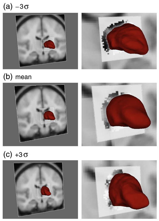
First mode of variation for the left thalamus. The first column shows the thalamus surface overlaid on the MNI152 template. The second column is a zoomed view, with the conditional mean intensity shown near the thalamus border, within the square patch. A lower position for the thalamus corresponds to an enlarged ventricle which correlates with the darker band of intensities at the thalamus border (due to more surrounding CSF). See text for a fuller explanation.

The following sections of this paper explain the details of the Bayesian Appearance Model (BAM), including our training set, provide validation experiments, and give an example application of vertex analysis for finding structural changes between disease and control cohorts.

Initial model construction

Training data

The training data used in this work consists of 336 pairs of images: the original T₁-weighted MR images of the brain and their corresponding manually-labelled counterparts. This dataset comprises six distinct groups of data and spans both normal and pathological brains (including cases of schizophrenia and Alzheimer’s disease). The size, age, group, and resolution for each group is given in Table 1, and the T₁-weighted image and manual labels of a single subject from the training set are depicted in Fig. 1. From the set of labelled structures we chose to model 15 structures: brainstem, the left/right amygdala, caudate nucleus, hippocampus, nucleus accumbens, putamen, pallidum and thalamus. Note that the brainstem model includes the fourth ventricle as it becomes very thin and excessively variable in the training data.

Table 1.

Groups within the training data and their respective size, age range and resolutions. NC indicates normal controls, SZ indicates schizophrenia, AD indicates Alzheimer’s disease, ADHD indicates attention deficit disorder and PC indicates prenatal cocaine exposure. For the first group we do not have demographics for all the subjects.

Group	Size	Age range	Resolution (mm)	Patient group
1	37	16 to 72	1.0×1.5×1.0	NC and SZ
2	42	18 to 87	1.0×1.0×1.0	NC and AD
3	17	65 to 83	0.9375×1.5×0.9375	NC and AD
4	87	23 to 66	0.9375×3.0×0.9375	NC and SZ
5	14	9 to 11	1.0×1.0×1.0	NC and PC
6	139	4.2 to 16.9	0.9375×1.5×0.9375	NC and ADHD and SZ

Fig. 1.

A coronal slice from a single subject’s images in the training set. a) MR T₁-weighted image. b) Manual segmentation overlaying the T₁-weighted image.

Linear subcortical registration

Prior to building the shape and intensity model, all data is registered to a common space based on the non-linear MNI152 template with 1×1×1 mm resolution (this is a template created by iteratively registering 152 subjects together with a non-linear registration method; Fonov et al. (2011)). The same registration procedure must be applied to both training images and any new images (to be segmented) so that they correctly align the new image and the model. Note that the shape variance we are modelling is the residual shape variance that exists after registration of all structures (jointly) to this template. Therefore the model is specific to the registration procedure, and in this case it removes the joint pose whilst retaining the relative pose of the individual structures.

A two-stage linear registration is performed in order to achieve a more robust and accurate pre-alignment of the subcortical structures. The first stage is an affine registration of the whole-head to the nonlinear MNI152 template using 12 degrees of freedom (DOF). The second stage, initialized by the result of the first stage, uses a subcortical mask or weighting image, defined in MNI space, to achieve a more accurate and robust 12 DOF registration to the MNI152 template. This subcortical mask contains a binary value in each voxel, and is used to determine whether that voxel is included or excluded from the calculation of the similarity function (correlation ratio) within this second stage registration. The mask itself was generated from the (filled) average surface shape of the 15 structures being modelled (using a 128-subject subset of the training subjects and the first stage affine registration alignments). The purpose of this mask is to exclude regions outside of the subcortical structures, allowing the registration to concentrate only on the subcortical alignment.

All linear registrations were performed using FLIRT (Jenkinson et al., 2002). For a new image, the two stage registration is first performed to get the image in alignment with the MNI152 template. Following this, the inverse transformation is applied to the model in order to bring it into the native space of this new image. This is advantageous as it allows the subsequent segmentation steps to be performed in the native space with the original (non-interpolated) voxel intensities.

Fitting the deformable model to the training labels

In our Bayesian appearance model, the individual shapes are modelled by deformable meshes that consist of sets of vertices connected by edges, and which are each topologically equivalent to a tessellated sphere. To build the model, a mesh is fit to each shape separately in each image of the training set, and the variation is modelled by a multivariate Gaussian distribution of the concatenated vector of vertex coordinates and intensity samples (more details in the Probabilistic model Section).

The first step in building the model from the training data is to generate the mesh parameterizations of all the manually labelled T₁-weighted images (training label images) while retaining point correspondence between meshes. Initially, each T₁-weighted image in the dataset (training intensity image) is registered to the non-linear-MNI152 (1 mm isotropic resolution) standard template using the linear registration procedure described previously. Then, for each structure and for each subject, a 3D mesh is fit to the binary image representing the manual label for that structure. The 3D mesh is initialized to the most typical shape (across subjects) and then deformed to fit the individual binary image. The desired cross-subject vertex correspondence is optimised by within-surface motion constraints and minimal smoothing within the 3D deformable model (Kass et al., 1988; Lobregt and Viergever, 1995; Smith, 2002).

The deformation process iteratively updates vertex locations according to a weighted sum of displacements: one image displacement and two regularisation displacements. The image displacement, d_n is in the direction of the surface normal, s_n, while the regularisation displacements, d_t and d_Amax, are both within the surface, along the directions s_t and s_Amax. These directions are defined as:

$$\mathbf{s}={\mathbf{v}}_0-\frac{1}{N}\sum _{i=1}^N{\mathbf{v}}_i,$$ (1a)

$${\mathbf{s}}_n=(\mathbf{s}·\widehat{\mathbf{n}})\widehat{\mathbf{n}},$$ (1b)

$${\mathbf{s}}_t=\mathbf{s}-{\mathbf{s}}_n,$$ (1c)

where n̂ is the local surface normal (unit vector) for the vertex v₀, N is the number of neighbouring vertices, v_i is the ith neighbouring vertex, s is the difference vector between the current vertex position and the average of its neighbours (in a regular grid there would be no difference), s_n and s_t are the normal and tangential components, respectively, of this difference vector, and s_Amax is the vector that bisects the largest adjacent triangle (see Fig. 2).

Fig. 2.

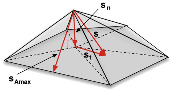
Illustration of the directions of the applied displacements: s_n is the normal vector; s_t is the surface tangent vector; and s_Amax is the bisector of the largest neighbouring triangle.

The external image displacement is along the inward/outward vertex normal and is given by,

$${\mathbf{d}}_n=\{\begin{array}{ll}-5\frac{{\mathbf{s}}_n}{\mid {\mathbf{s}}_n\mid }\hfill & \text{if}\mathit{label}=1,\hfill \\ +1\frac{{\mathbf{s}}_n}{\mid {\mathbf{s}}_n\mid }\hfill & \text{if}\mathit{label}=0,\hfill \end{array}$$ (2)

where label is the binary image value, s_n is the surface normal as defined by Eq. (1b) and the coefficients −5 and 1 were chosen based on empirical stability in order to fit the surface closely to the labelled edge. Note that the choice of form for the displacement here is specific to the training set and structures modelled, and only affects this initial model-building phase.

The first regularisation displacement is tangential to the surface and is applied in order to favour an even point density across the surface — Eq. (3). This regularisation displacement is identical to that used by BET (Smith, 2002), except that its weighting is initially set to zero and adaptively updated, in order to try to retain better vertex correspondence across subjects. If the surface self-intersects during the deformation process, the process is reset and the regularisation displacement is given more weight. Self-intersection is detected by testing for triangle–triangle intersection between any pair of triangles within the surface. This iterative update aims to apply a minimal amount of within-surface motion, since within-surface motion is likely to reduce the cross-subject correspondence of vertices, although for large changes in shape some within-surface motion is still necessary. Since the true correspondence within the surface is unknown we assume that a mapping with minimal within-surface change gives a better approximation to the true correspondence.

A second regularisation displacement is also applied in order to increase the stability of the deformation process. This displacement moves the vertices so as to favour equal area triangular patches and it acts along the line that bisects the largest neighbouring triangle —Eq. (4). These regularisation displacements are defined as:

$${\mathbf{d}}_t={\mathbf{s}}_t,$$ (3)

$${\mathbf{d}}_{\mathit{Amax}}=A_{\mathit{max}}\frac{{\mathbf{s}}_{\mathit{Amax}}}{\mid {\mathbf{s}}_{\mathit{Amax}}\mid },$$ (4)

where s_t is the surface tangent vector (Eq. (1c)), s_Amax is the bisector of the largest neighbouring triangle (Fig. 2), and A_max is the largest area of the adjacent triangular patches.

Note that the deformable model displacements described here are only required when fitting surfaces to the manual labels as part of the model building process. Once the models are built, the fitting of structures in new images is done by optimising the probabilities based on the intensities and the model (see later). Therefore these displacements are not used in any way when performing the subsequent segmentations except insofar as they define the model. Furthermore, the different stages in building the model were all carefully manually inspected to ensure that the surface lay within one voxel of the manually defined boundary, with the magnitude of the displacements tuned as necessary to obtain good fits to the individual datasets. This manual tuning was only occasionally necessary and, in general, the weights used for the displacements had little effect on the model fit compared to the inter-subject variation in the training data. Therefore, because the displacements and weights were only used to create the model, and this is dominated by the inter-subject variation, the influence of the weights on the final segmentation results was not considered further.

Finally, appearance is modelled using normalised intensities that are sampled, for each subject, from the corresponding training intensity image along the surface normal at each vertex of the training mesh (both inside and outside the surface). There are 13 samples taken per vertex, sampled at an interval of half the standard-space voxel resolution (i.e., 0.5 mm); this was chosen based on the empirically observed performance of the Bayesian Appearance Model, although we have not found it to be highly sensitive to these parameters. The normalisation of the intensities is done in two stages: (1) by applying a global scaling and offset to the intensities in the whole image such that the 2nd and 98th percentiles are rescaled to 0 and 255 respectively, and (2) by subtracting the mode of the intensities within a specified structure. In the second stage it is usually the mode of the intensities in the structure being modelled that is subtracted, however there is also the option of using a nearby structure instead. The effect of the structure used to normalise the intensity is explored in the Results and discussion Section.

Probabilistic model

Our model is trained from a limited set of mesh vertices and intensity samples that correspond to the limited set of volumetric training data. We treat all training data as column vectors, either of concatenated vertex coordinates or coordinates and corresponding intensity samples. For example, for a 2D rectangle parameterized by the corner vertices = {(−2, 0), (−2, 3), (3, 3), (3, 0)} the training vector for shape alone would be x_i =[−2 0−2 3 3 3 3 0]^T. It is essential that vertex correspondence (consistent ordering) is maintained across all the training data. To include intensity data, the training vector would have the concatenated intensity samples, in a consistent order, added after the vertex coordinates. We will find it helpful later on to partition the vectors into separate shape and intensity parts.

Initially, we present the model in its most general form, without restricting the training vectors to be of any particular form. This is useful since it allows us to use the model later on for shape, shape–intensity or multiple shape (and intensity) modelling. To begin with we assume that we have a limited set of training data, denoted by = {x₁…x_ns}, where each observation comes from an underlying multivariate Gaussian distribution:

$$\begin{array}{l}p({\mathit{x}}_i\mid \mathbf{\mu },\mathbf{\lambda })=N_k({\mathit{x}}_i\mid \mathbf{\mu },\mathbf{\lambda })\\ ={\mathbf{\lambda }}^{\frac{1}{2}}{(2\pi )}^{\frac{-k}{2}}\mathit{exp}\left(-\frac{1}{2}{({\mathit{x}}_i-\mathbf{\mu })}^T\mathbf{\lambda }({\mathit{x}}_i-\mathbf{\mu })\right),\end{array}$$ (5)

where n_s is the number of training samples, k is the dimensionality of a vector x_i, μ is the mean and λ is a k×k positive-definite precision matrix. The precision matrix is equal to the inverse of the covariance matrix, Σ. N_k is the k-dimensional multivariate Gaussian distribution.

For the purposes of shape and intensity modelling we want to know what the distribution is for a new observation, given what information is available in the training data. To do this we start by using the multivariate Gaussian model and derive the distribution of the mean and precision given the previously observed training data. We then perform a marginalisation over the mean and precision to obtain a distribution for the new observation given the training data. That is:

$$\begin{array}{l}p({\mathit{x}}_{\mathit{obs}}\mid \mathcal{Z},\theta )=\int p({\mathit{x}}_{\mathit{obs}}\mid \mu ,\mathbf{\lambda })p(\mathbf{\mu },\mathbf{\lambda }\mid \mathcal{Z},\theta )d\mathbf{\mu }d\mathbf{\lambda }\\ \propto \int p({\mathit{x}}_{\mathit{obs}}\mid \mathbf{\mu },\mathbf{\lambda })p(\mathcal{Z}\mid \mathbf{\mu },\mathbf{\lambda })p(\mathbf{\mu },\mathbf{\lambda }\mid \theta )d\mathbf{\mu }d\mathbf{\lambda },\end{array}$$ (6)

where x_obs is a new observation (image) sampled from the same distribution as that of the datasets in , and θ represents a set of hyperparameters associated with the prior distribution for μ and λ.

The final form for this distribution can be arrived at by straightforward probabilistic calculations and the selection of a non-informative prior (Appendix A shows the detailed calculations). The resulting form is:

$$p({\mathit{x}}_{\mathit{obs}}\mid \mathcal{Z},\epsilon )={St}_k\left({\mathit{x}}_{\mathit{obs}}\mid \overline{\mathit{x}},{\left(\frac{\mathit{S}+2{\epsilon }^2\mathit{I}}{n_s-1}\right)}^{-1},n_s-\frac{1}{n_s}\right),$$ (7)

where St_k is a multivariate Student distribution in k dimensions (defined in Appendix A, Eq. (A.10)), x̄ is the sample mean of the training vectors, S=ZZ^T is the un-normalised sample covariance matrix of the training vectors, with Z being the matrix formed from all the demeaned training (column) vectors, and ε is a scalar hyperparameter relating to prior (unseen) variance.

Specification of the prior variance

The prior distributions specify information, or beliefs, about the shape and intensities before the training data are seen. As we want the training data to specify as much information as possible, and we do not wish to introduce any bias, we used non-informative priors. See Appendix A for full details.

The general non-informative prior leaves a single hyperparameter, ε², to be specified. This can be interpreted as the variance associated with the variation in shape (and/or intensity) that is not captured by the limited training set. One way of specifying this value is to use empirical Bayes and estimate it from the limits of the variances contained in the training data (e.g., a fraction of the lowest eigenvalues or of the total observed variance). Note that the addition of the scaled identity matrix is analogous to ridge regression (Hastie et al., 2001), where a scaled identity matrix is added to the covariance matrix estimate, and has been used in the context of shape models previously (Cremers et al., 2002). This broadens the distribution, reflecting unseen variations in the population, and here it arises naturally as a consequence of needing to specify an unbiased prior distribution of shape (and/or intensity).

Although an exact prescription for setting the ε parameter is not provided by this framework, sensible limits can easily be established (e.g., in terms of the fraction of total variance). Furthermore, its effect is generally small and reduces as the size of the training set increases. In fact, it is not even required if there are more training datasets than parameters. This is in contrast to the weightings between forces or shape–intensity relations, as used by other approaches (Cootes and Taylor, 2001; Heimann and Meinzer, 2009; Lobregt and Viergever, 1995; Montagnat et al., 2001; Pitiot et al., 2004; Shen et al., 2011), as they typically have a significant effect on the results, independent of the size of the training set, without necessarily obvious ways to interpret or set their values.

Conditional distributions

Within this framework we can also utilise shape–intensity or shape–shape relationships which are useful, for example, in finding the shape boundary given the observed image intensities (which is the typical segmentation problem) or to hierarchically determine the boundary of one shape given the boundary of another. It is the conditional probability distributions across partitions of the full multivariate Gaussian model which give information about these relationships.

A partition of x is a subset, x_j, corresponding to a particular attribute j (e.g. shape, intensity, etc.). In the case of our training data, each partition will still have the same number of samples n_s, and in our application we partition the data into either shape and intensity or into different shapes. The conditional distribution for shape given intensity is essential for segmenting new images.

The partitioning is defined such that

$$\mathbf{x}=({\mathbf{x}}_1,{\mathbf{x}}_2)$$ (8a)

$$\mathbf{\mu }=({\mathbf{\mu }}_1,{\mathbf{\mu }}_2)$$ (8b)

$$\mathbf{\lambda }=\left[\begin{array}{cc}{\mathbf{\lambda }}_{11}& {\mathbf{\lambda }}_{12}\\ {\mathbf{\lambda }}_{21}& {\mathbf{\lambda }}_{22}\end{array}\right]={\left[\begin{array}{cc}{\mathbf{\sum }}_{11}& {\mathbf{\sum }}_{12}\\ {\mathbf{\sum }}_{21}& {\mathbf{\sum }}_{22}\end{array}\right]}^{-1}$$ (8c)

$$k=k_1+k_2$$ (8d)

where k_j is the dimensionality of the jth partition, so that can be partitioned in the same manner, with = ( , ), where = {x̃_ij…x̃_nsj}, with the first subscript denoting image number (within the training dataset) and the second the shape partition. For example, the first partition, , could be the concatenated vertex coordinates (shape) across all the training images and the second, , could be the corresponding intensity samples across all the training images. Alternatively, for shape–shape relationships (e.g., the caudate given the known location and shape of the thalamus), the first partition could consist of the concatenated vertex coordinates of the structure of interest (caudate) and the second partition consist of the concatenated vertex coordinates of the predictive structure (thalamus).

The conditional distribution can be written as

$$\begin{array}{l}p({\mathit{x}}_1\mid {\mathit{x}}_2,\mathcal{Z},\epsilon )=\frac{p({\mathit{x}}_1,{\mathit{x}}_2\mid \mathcal{Z},\epsilon )}{p({\mathit{x}}_2\mid \mathcal{Z},\epsilon )}\\ ={St}_{k_1}({\mathit{x}}_1\mid {\mathbf{\mu }}_{1\mid 2},{\mathbf{\lambda }}_{1\mid 2},{\alpha }_{1\mid 2}),\end{array}$$ (9a)

using standard algebraic manipulations of the multivariate Student distribution (see Bernardo and Smith, 2000), and with

$${\mathbf{\mu }}_{1\mid 2}={\mathbf{\mu }}_1-{\mathbf{\lambda }}_{11}^{-1}{\mathbf{\lambda }}_{12}({\mathit{x}}_2-{\mathbf{\mu }}_2),$$ (9b)

$${\mathbf{\lambda }}_{1\mid 2}={\mathbf{\lambda }}_{11}\left[\frac{{\alpha }_{1,2}+k_2}{{\alpha }_{1,2}+{({\mathbf{x}}_2-{\overline{\mathbf{x}}}_2)}^T{\mathbf{\sum }}_{22}^{-1}({\mathbf{x}}_2-{\overline{\mathbf{x}}}_2)}\right],$$ (9c)

$${\alpha }_{1\mid 2}=n_s-\frac{1}{n_s}+k_2\text{and}{\alpha }_{1,2}=n_s-\frac{1}{n_s}.$$ (9d)

For a partitioned covariance matrix we define the prior covariance, β, to be a piecewise-scaled identity matrix

$$\mathbf{\beta }=\left[\begin{array}{cc}{\epsilon }_1^2\mathbf{I}& 0\\ 0& {\epsilon }_2^2\mathbf{I}\end{array}\right],$$

where ${\epsilon }_j^2$ is the error variance corresponding to the jth partition. Thus for each partition a different error variance, ${\epsilon }_j^2$, may be used, giving λ= (n_s−1)(S + 2β)⁻¹ as in Eq. (7).

Parameterization of the model

In our method it is extremely useful to parameterize the space of shapes (and/or intensities) using the mean and eigenvectors of the training set, which is naturally related to the multivariate Gaussian model. This has significant implications for simplifying the expressions and massively reducing computational cost.

The eigenvectors are related to the un-normalised sample covariance matrix (see Eq. (7)) by S=ZZ^T=UDD^TU^T, using the SVD of Z=UDV^T. We therefore parameterize our data in the same way as for the standard shape and appearance models, which is

$$\mathit{x}=\mathbf{\mu }+\mathit{U}\frac{{\mathit{D}}_{\epsilon }\sqrt{\gamma }}{\sqrt{n_s-1}}\mathit{b},$$ (10)

where μ = x̄ is the mean vector across the training set; the matrix D_ε is a diagonal matrix such that ${\mathit{D}}_{\epsilon }^2$ consists of the eigenvalues (correspondingly ordered) of S+2ε²I; the scalar $\gamma =(n_s-n_s^{-1})/(n_s-n_s^{-1}-2)$; and b is the model parameter vector that weights the linear combination of eigenvectors, U. The elements of b are scaled so that they indicate the number of standard deviations along each mode, such that

$${(\mathit{x}-\mathbf{\mu })}^T{\mathbf{\sum }}^{-1}(\mathit{x}-\mathbf{\mu })={\mathit{b}}^T\mathit{b}\gamma ,$$ (11)

which is used to simplify many equations. Note that this parameterization is most usually applied to the shape partition alone but can also be applied to shape and intensity, or just intensity.

Bayesian appearance models

To formulate the Bayesian Appearance Model we take the general mathematical framework developed in the previous sections and apply it to intensity and shape partitions: x_I and x_s. The shape partition is modelled using Eq. (10), so that given the intensities from a new image, the vector b_s (new shape instance) can be estimated from the posterior conditional distribution p(x_s |x_I, ).

In the following sections we describe how the model is fit to new data. As discussed earlier, when fitting to the new data, the model is first registered into the native space using the inverse transform. This transform is applied only to the average shape and eigenvectors. One slightly unusual consequence of the joint registration of all shapes is that not all pose (orientation) is removed from every structure. That is, pose differences are contained in the eigenvectors although, in practice, the residual pose differences are small because the initial linear registration removes the overall joint pose of all the structures. This residual pose represents changes in the relative pose between different structures and may be of interest. However, there is no restriction within the framework that prevents the individual pose from being completely removed, if desired.

Posterior as a similarity function

The conditional posterior probability, p(x_s |x_I, ), measures the probability and hence the goodness of fit for a proposed segmentation. We want to maximise this probability with respect to the shape model parameters b_s. Simplifying this posterior, and expressing it in terms of its logarithm, we can obtain the following

$$lnp({\mathbf{x}}_s\mid {\mathbf{x}}_I)=C+\frac{1}{2}ln\left(\frac{{\alpha }_{I,s}+k_s}{{\alpha }_{I,s}+{\mathbf{b}}_s^T{\mathbf{b}}_s{\gamma }_s}\right)-\frac{({\alpha }_s+k_s)}{2}ln\left(1+\frac{1}{{\alpha }_s}{\mathbf{b}}_s^T{\mathbf{b}}_s{\gamma }_s\right)-\frac{({\alpha }_{I,s}+k_s+k_I)}{2}ln\left(1+\frac{1}{{\alpha }_{I,s}+{\mathbf{b}}_s^T{\mathbf{b}}_s{\gamma }_s}{({\mathbf{x}}_I-{\mathbf{\mu }}_{I\mid s})}^T{\mathbf{\lambda }}_{\mathit{cII}}({\mathbf{x}}_I-{\mathbf{\mu }}_{I\mid s})\right)$$ (12)

where C is a constant, ${\alpha }_{I,s}={\alpha }_s=n_s-n_s^{-1},{\gamma }_s=(n_s-n_s^{-1})/(n_s-n_s^{-1}-2)$, k_I, and k_s are the respective dimensionalities of the intensity and shape partitions (k_I =13n_vert and k_s =3n_vert for our implementation, where n_vert is the number of vertices and 13 is chosen to sample an intensity profile at each vertex that extends for ±3 mm in steps of 0.5 mm, as discussed at the end of Fitting the deformable model to the training labels Section) and x_I is the vector containing the observed intensities. The quantities λ_cII (the un-scaled conditional precision matrix) and μ_I|s (the conditional mean given shape) are defined in Appendix B, where it is also shown how the different terms in this posterior can be calculated efficiently.

Optimization

To maximise the similarity function (the posterior probability) a conjugate gradient descent search scheme is employed (Press et al., 1995). Since we parameterize the shape space by the mode parameters, b_s, we are searching along the eigenvectors, or modes. As the eigenvectors are ordered by descending variance, the lower modes contribute less information to the model (or even just noise) compared to the upper modes. Consequently, since lower modes increase the dimensionality of the search space, making the optimization more difficult, as well as increasing computational time, it can be beneficial to truncate the number of modes considered. We have found that there is an optimal number of modes to include in order to get the best performance, which is confirmed empirically (see the Results and discussion Section).

Computational simplifications

To make this model computationally feasible in practice it is necessary to eliminate all operations on k×k matrices. This is because the calculation of the inverse of the full k×k covariance matrix is extremely computationally expensive (as typically k >10, 000), whereas by exploiting the low rank (n_s =336) of the sample covariance matrix, the computations can be considerably simplified. This makes the calculations feasible in terms of time and memory requirements. In this way we combine the benefits of having well-defined (full rank) inverses, due to the additional scaled-identity matrix, and the computational efficiency of working with the low-rank sample covariance.

Evaluations of the relevant terms for the posterior probability, including conditional probabilities, can be simplified so that only n_s × n_s, n_s × k₁, n_s ×1 and k₁ ×1 matrices need to be used. Appendix B details the main computational simplifications.

Boundary correction

In the preceding sections we model shape with a mesh model, parameterized by the coordinates of its vertices. However, it is often necessary, or desirable, to create volumetric (voxelated) masks that represent the structure segmentation. Therefore, there is a need to convert between the mesh-based and volumetric representations of a segmented structure.

We create a volumetric output from the mesh by the following steps: (i) identifying the voxels through which the mesh passes (i.e., partially filled voxels); (ii) marking these voxels in a volumetric image as the boundary voxels; (iii) filling the interior of this boundary. Once this is done we need a way to classify whether each boundary voxel should remain part of the segmentation or not (if a binary segmentation is required). For this step we have explored several classification methods and found that one based on the results of a 3-class classification of the intensities (grey matter, white matter and CSF) using the FSL/FAST method (Zhang et al., 2001) performs the best overall. A rectangular ROI that encompasses the structure of interest (extended by two voxels) is used as input to the FAST method, which models the intensity distribution as a Gaussian mixture-model in addition to a Markov Random Field. We use this method of boundary correction for most of the rest of this paper. It is also worth noting that other boundary correction methods could easily be used with our implementation, as this is not core to the Bayesian Appearance Model in any way.

There are three exceptions to the use of the FAST-based boundary correction method. These are for the putamen, pallidum and thalamus where a slightly different surface model was fit. In these cases the surfaces were fit to a slightly eroded version of manual labels (at the surface parameterization phase) such that the eroded edge was inset by 0.5 mm from the outer boundary of the manual labels. For these structures applying no thresholding and simply including all the boundary voxels in the final volumetric output gives good results. This is referred to as a boundary correction of “none” in Table 3 and is compared, for these structures, with the FAST-based boundary correction. Note that this different surface model was also tried for the other structures but was found to be significantly worse, and sometimes problematic, compared to the standard surface fitting.

Vertex analysis

The output from a subcortical segmentation method can be used in many ways; one application is to look for differences in these structures between different groups (e.g., disease versus healthy controls). Many such group difference studies have been carried out based on volumetric measures of the structures of interest (e.g., caudate, hippocampus, etc.). However, volumetric studies do not show where the changes are occurring in the structure, and this may be of critical importance when investigating relationships with neighbouring structures, connectivity with more distant structures, or changes in the different subcortical nuclei within the structure.

Local changes can be directly investigated by analysing vertex locations, which looks at the differences in mean vertex position between two (or more) groups. This type of analysis does not require boundary correction to be performed, as it works directly with the vertex coordinates (in continuous space) of the underlying meshes. The Vertex Analysis is performed by carrying out a multivariate test on the three-dimensional coordinates of corresponding vertices. Each vertex is analysed independently, with appropriate multiple-comparison correction methods (e.g., FDR or surface-based cluster corrections) performed later, as is the case for standard volumetric image analysis.

The coordinates for each vertex can either be analysed directly in standard space (where the models are generated) or can be mapped back into any other space (e.g., group mean). Moreover, changes in pose (global rotation and translation) between different subjects are often of no interest, and these can be removed by a rigid alignment of the individual meshes, if desired. For this purpose we have implemented an alignment based on minimising the sum of square error surface distance for the mesh coordinates.

Once the coordinates are appropriately transformed, a multivariate F-test is performed for each vertex separately using the MultiVariate General Linear Model (MVGLM) with Pillai’s Trace as the test statistic. The details can be found in Appendix C. By implementing a general linear model it is also possible to investigate more complex changes, not just the mean difference between two groups. For instance, it is possible to jointly look at the effect of age and disease with a MANCOVA design, which is easily implemented within the MVGLM. Whatever the design, the F-statistics that are formed are sensitive to changes of the coordinates in any direction. To differentiate between the different directions (e.g., atrophy versus expansion) it is necessary to use the orientations of the vectors, particularly the difference of the mean locations, to disambiguate the direction of the change.

Certain localised changes in brain structures can also be detected using other methods, such as voxel-based morphometry (VBM). However, with VBM the inference is based on locally-averaged grey-matter segmentations and is therefore sensitive to the inaccuracies of tissue-type classification and arbitrary smoothing extents. The vertex analysis method, however, utilises the joint shape and appearance model to robustly determine the structural boundary, and so is purely local, being based directly on the geometry/location of the structure boundary. Therefore it has the potential to localise changes more precisely, as there is no additional smoothing and it directly measures changes in geometry.

Results and discussion

In this section we test the Bayesian Appearance Model both qualitatively and quantitatively on real MRI data. This includes a set of leave-one-out (LOO) cross-validation tests comparing volumetric overlap with the manual labelled images from the training set. In addition, vertex analysis is tested by comparing cohorts of patients with matched healthy controls.

All the results shown here use a C++ implementation of the Bayesian Appearance Model that is distributed as part of FSL (Woolrich et al., 2009), where it is called FIRST (FMRIB’s Integrated Registration and Segmentation Tool). The run time for FIRST on a modern desktop, with default parameters, is approximately 5 min (for linear registration) plus 1 min per structure being segmented.

Before showing the testing and validation results we will illustrate the changes captured by the Bayesian Appearance Model. Fig. 3 shows the change in shape and conditional intensity distribution as the shape parameters vary along one of the individual modes of variation. It shows a graphical depiction of ±3 standard deviations along the first mode of variation for the left thalamus and the conditional intensity mean associated with it; the shape is shown overlaid on the MNI152 template in each case. The first mode is predominantly associated with translation, where the translation typically correlates with an increased ventricle size, which is reflected in the fact that for enlarged ventricles (lower thalamus position) there is an enlarged dark band above the thalamus in the conditional mean intensity, corresponding to the extra surrounding CSF. In contrast, when the thalamus is in a higher position, correlated with smaller ventricles, the conditional mean intensity is brighter, consistent with the higher prevalence of white matter nearer to the thalamic border. The intensities in this latter case are close to the white-matter mean values as the partial volume fraction of the CSF for the datasets with the smallest ventricles is very low across much of the superior thalamus border. Furthermore, the conditional distribution captures the changing variance of the intensities for different shapes.

Validation and accuracy

Leave-one-out tests

To quantitatively evaluate the accuracy of the algorithm, a Leave-One-Out (LOO) cross-validation method was used across the 336 training sets. For all evaluations the manual segmentations were regarded as the gold standard, and the segmentation performance was measured using the standard Dice overlap metric:

$$D=\frac{2TP}{2TP+FP+FN},$$ (13)

where TP is the true positive (overlap) volume, FP is the false positive volume and FN is the false negative volume.

The LOO tests were run independently for all 15 subcortical structures. For each structure, the LOO test selects each image, in turn, and segments it using a model built from the remaining 335 images. All tests used the following empirically-tuned parameters: the prior constants ε_i and ε_s were both set to 0.0001% of the total variance in the training set; the number of modes included in the fitting were chosen based on the mean Dice overlaps across modes of variation (as seen in Fig. 6) and correspond to the number of modes indicated in Table 3; and the FAST-based boundary correction was applied to all structures except the thalamus and pallidum where all boundary voxels were included. Fig. 4 shows an example of the segmentation of one image (for all of the 15 structures) from the LOO test, while Fig. 5 shows the results of the quantitative Dice overlap measure, and Table 3 shows the mean Dice values broken down by group.

Fig. 6.

The mean Dice overlap between the filled surfaces and the manual labels for each of the 15 structures when restricting the fitting to 20, 30, 40, 50, 60, 70, 80, 90 and 100 modes of variation (in different colours — see key on the right hand side). All structures used the FAST method for boundary correction and had both prior constants ε_i and ε_s as specified in Table 2.

Table 3.

Mean and standard deviation of Dice overlap for each group, using the number of modes of variation and priors as specified in Table 2 (number of modes chosen using Fig. 6).

Structure	B. corr. method	Int. ref.	Group 1	Group 2	Group 3	Group 4	Group 5	Group 6
Brain stem	FAST	Self	0.855 (0.0193)	0.855 (0.0175)	0.86 (0.0146)	0.808 (0.0254)	0.848 (0.0216)	0.832 (0.0248)
L. N. accumbens	FAST	Self	0.738 (0.0482)	0.729 (0.0595)	0.7 (0.0852)	0.728 (0.063)	0.679 (0.0711)	0.707 (0.0703)
L. amygdala	FAST	Thal.	0.731 (0.0809)	0.772 (0.0493)	0.747 (0.0657)	0.735 (0.0513)	0.74 (0.0653)	0.742 (0.0654)
L. amygdala	FAST	Self	0.734 (0.0785)	0.769 (0.0554)	0.747 (0.0673)	0.73 (0.0524)	0.744 (0.0628)	0.74 (0.0645)
L. caudate	FAST	Thal.	0.861 (0.0288)	0.853 (0.0454)	0.88 (0.0291)	0.85 (0.0319)	0.871 (0.0212)	0.847 (0.0309)
L. caudate	FAST	Self	0.859 (0.0297)	0.852 (0.042)	0.881 (0.0275)	0.849 (0.0308)	0.871 (0.0214)	0.846 (0.0307)
L. hippocampus	FAST	Thal.	0.796 (0.0663)	0.834 (0.0333)	0.840 (0.0214)	0.803 (0.0.0289)	0.804 (0.0168)	0.813 (0.0304)
L. hippocampus	FAST	Self	0.796 (0.0614)	0.832 (0.0336)	0.838 (0.0209)	0.802 (0.0298)	0.803 (0.0161)	0.812 (0.0304)
L. pallidum	None	Self	0.821 (0.035)	0.795 (0.0648)	0.769 (0.0258)	0.78 (0.0379)	0.769 (0.0474)	0.815 (0.0355)
L. pallidum	FAST	Self	0.799 (0.0363)	0.764 (0.0738)	0.765 (0.0293)	0.723 (0.0516)	0.761 (0.0426)	0.795 (0.0421)
L. putamen	None	Self	0.877 (0.0196)	0.874 (0.0262)	0.845 (0.0275)	0.869 (0.0198)	0.853 (0.0153)	0.884 (0.0194)
L. putamen	FAST	Self	0.898 (0.0151)	0.872 (0.0236)	0.864 (0.0337)	0.888 (0.0194)	0.846 (0.0141)	0.887 (0.0202)
L. thalamus	None	Self	0.888 (0.0182)	0.884 (0.0203)	0.852 (0.0218)	0.854 (0.0237)	0.891 (0.0287)	0.893 (0.0171)
L. thalamus	FAST	Self	0.868 (0.0225)	0.87 (0.0209)	0.869 (0.0261)	0.852 (0.0188)	0.875 (0.0174)	0.865 (0.0199)
R. N. accumbens	FAST	Self	0.695 (0.0604)	0.698 (0.0736)	0.645 (0.125)	0.728 (0.074)	0.663 (0.0742)	0.694 (0.0693)
R. amygdala	FAST	Thal	0.719 (0.0723)	0.771 (0.0468)	0.771 (0.0529)	0.727 (0.0513)	0.755 (0.0434)	0.746 (0.0598)
R. amygdala	FAST	Self	0.725 (0.0719)	0.763 (0.0549)	0.770 (0.0559)	0.724 (0.0558)	0.741 (0.0425)	0.743 (0.0607)
R. caudate	FAST	Thal.	0.818 (0.0307)	0.851 (0.0253)	0.868 (0.0289)	0.816 (0.0346)	0.798 (0.0407)	0.836 (0.0293)
R. caudate	FAST	Self	0.818 (0.029)	0.831 (0.0583)	0.854 (0.0394)	0.816 (0.0364)	0.801 (0.0466)	0.835 (0.029)
R. hippocampus	FAST	Thal.	0.801 (0.0566)	0.84 (0.0315)	0.844 (0.0193)	0.8 (0.0336)	0.804 (0.0186)	0.809 (0.0284)
R. hippocampus	FAST	Self	0.8 (0.0552)	0.836 (0.0363)	0.841 (0.0257)	0.8 (0.0326)	0.805 (0.017)	0.807 (0.0303)
R. pallidum	None	Self	0.799 (0.0405)	0.799 (0.0437)	0.762 (0.035)	0.773 (0.046)	0.757 (0.0465)	0.81 (0.0392)
R. pallidum	FAST	Self	0.769 (0.0449)	0.786 (0.0325)	0.749 (0.0456)	0.719 (0.0544)	0.754 (0.0421)	0.789 (0.0442)
R. putamen	None	Self	0.874 (0.0282)	0.878 (0.0217)	0.847 (0.026)	0.864 (0.0211)	0.863 (0.0138)	0.886 (0.0194)
R. putamen	FAST	Self	0.883 (0.0251)	0.87 (0.0235)	0.857 (0.0311)	0.875 (0.0252)	0.873 (0.0182)	0.885 (0.0223)
R. thalamus	None	Self	0.889 (0.0205)	0.887 (0.0209)	0.86 (0.0227)	0.859 (0.0236)	0.892 (0.0215)	0.894 (0.0191)
R. thalamus	FAST	Self	0.865 (0.0192)	0.867 (0.0233)	0.866 (0.0283)	0.85 (0.0189)	0.874 (0.0101)	0.859 (0.0209)

Fig. 4.

Example of a subcortical segmentation from the LOO tests, as described in the text.

Fig. 5.

Boxplots of the Dice overlap between the filled surfaces and the manual labels for each of the 15 structures. All structures were segmented using the number of modes of variation and both prior constants ε_i and ε_s, as specified in Table 2. The prior constants are defined as a percentage of the total variance in the training set. The FAST-based method was used for boundary correction, with the exception of the thalamus and pallidum where all voxels were included (see text).

The Dice results obtained are generally comparable to or better than those reported by other methods (Babalola et al., 2008; Carmichael et al., 2005; Fischl et al., 2002; van Ginneken et al., 2007; Morey et al., 2009; Pohl et al., 2007). For example, in Morey et al. (2009) similar results overall were found for ASEG (Fischl et al., 2002) and our Bayesian Appearance Model for the hippocampus and the amygdala, although in that paper a simpler method of boundary correction was used, rather than the FAST-based approach which we have more recently found to be superior. In Pohl et al. (2007) a hierarchical model is used to segment the amygdala and hippocampus, in a mixed pathology dataset, with superior performance for the amygdala but nearly identical performance for the hippocampus. Results of evaluating caudate segmentations across many different methods can be found as part of the ongoing “Caudate Segmentation Evaluation” (http://www.cause07.org; van Ginneken et al., 2007) which give values less than 80%, while our Dice results are often above 80%, although their results are averages over five different metrics and the data involves paediatric images (younger than any in our training set), and so cannot be directly compared with the results given here. In general, accurately measuring the relative performance of different methods over a rich set of subcortical structures will require conducting a specific and thorough study using the same data for all methods, which is beyond the scope of this paper.

The results of the Bayesian Appearance Model show that the best structures in terms of Dice overlap are the putamen and the thalamus, while in contrast, the worst structures are the nucleus accumbens and the amygdala, being between 0.1 and 0.2 lower in their median Dice overlap. However, the spread of results differs greatly between all the structures, with the accumbens, amygdala, hippocampus and pallidum showing a greater spread, with some relatively poor performances, whereas the putamen and thalamus show quite a tight range of high Dice overlaps.

For small structures, such as the nucleus accumbens, or structures with large surface-area-to-volume ratios, such as the caudate, the Dice overlap measure heavily penalises small differences in surface error, since an average error of one voxel at the boundary will substantially affect the volume overlap. By comparison, structures such as the thalamus, which are larger and have a lower surface-area-to-volume ratio, are less affected by small differences in boundary position. Therefore it is expected that, for example, the nucleus accumbens would perform worse than the thalamus due to its small size. However, these tendencies do not explain all of the features of the results, and the variability of the structure’s shape and intensity characteristics also play an important role.

There are many factors that might affect the ability of the method to perform well, such as: the ability of the multivariate Gaussian model to correctly represent the true shape/intensity probabilities; the ability of the optimization method to converge on the globally optimal solution; mismatches between the real underlying ground truth and the manual labellings; errors at the boundary due to the necessity to produce binary segmentations for comparison with the binary manual labels; the number of modes used in the fitting; and so on. Of these factors, there are some that we have direct control over (e.g. the number of modes used) and these can play an important part in the fitting process. The effects that these have are investigated next.

Effect of the number of modes of variation

To start with we investigate the dependence of the results on the number of modes included in the fitting process. This was done by repeating the entire LOO test using fitting that was restricted to 20, 30, 40, 50, 60, 70, 80, 90 and 100 modes. Fig. 6 shows these results as a Dice overlap measure for each structure and for the different number of modes (eigenvectors) that were included.

The number of modes of variation retained in the fitting has an impact on the amount of detail that may be captured using the model, but the results did not vary strongly with the number of modes included. The main structures where it had a noticeable effect were the amygdala and brainstem. In both cases, including more modes increased the Dice overlap, but each appeared to reach a plateau with around 80 to 100 modes. Therefore, the results are not highly sensitive to the choice of the number of modes used for each structure. Consequently, we believe that the values specified in Table 2 can be used quite generally and provide a good compromise between including enough variation to capture the structural detail, and avoiding too many modes which can make the optimization difficult and significantly increase computational cost.

Table 2.

Number of modes of variation used and choice of priors for shape and intensity (as percent of variance) for each structure used for LOO cross-validation.

Structure	Number of modes	εs(%)	εI (%)
L/R N. accumbens	50	0.01	0.001
L/R amygdala	80	0.01	0.01
L/R caudate	40	0.01	0.001
L/R hippocampus	30	0.01	0.01
L/R pallidum	40	0.01	1.0
L/R putamen	40	0.001	0.1
L/R thalamus	40	0.01	1.0
Brain stem	90	0.01	0.001

Results on sub-groups

The second investigation of the sensitivity of the method was made by looking at the performance for the separate sub-groups in the training set, since they have different image resolution, signal-to-noise ratio, and contrast-to-noise. The results are shown in Table 3 (demographics and image resolution for each group are shown in Table 1). The overlap is shown using 80 modes of variation since, for all structures, the Dice overlap (in Fig. 6) reached a plateau by this number. The prior constants and boundary correction were the same as specified previously.

It can be seen in Table 3 that there is little difference in the Dice results between the groups, despite the range of resolutions and general image quality. In particular, group 4, which has a slice thickness of 3 mm, does not perform noticeably worse than other groups, where the slice thickness is between 1.0 and 1.5 mm. There is also little effect evident when changing the structure used to provide the intensity normalisation (the intensity reference structure). In most cases the structure acts as its own reference, by subtracting the mode of the intensity distribution. However, for small structures, using a larger structure like the thalamus, as a local reference can reduce the number of poor performing outlier segmentations, even though the mean performance is largely unaffected. In contrast, comparing the FAST-based boundary correction method with no correction (including all the boundary voxels) for the pallidum, putamen and thalamus, showed a small systematic improvement in favour of no correction. This was not the case for the other structures (data not shown).

Sensitivity to priors

The third investigation of sensitivity of the method involved varying the parameters ε_s and ε_I. These were both chosen to be fractions of the total estimated shape and intensity variances respectively. They was chosen empirically, based on examination of the model’s performance over a range of the parameter values, all of which were small fractions of the total variance, so that the model depends almost entirely on the training data. This empirical approach to setting the parameter values is common to many medical imaging problems (Friston et al., 2002). Although the choice of ε is not a proven, optimal solution, it provides a simple, practical solution to a complex (poorly conditioned inverse covariance) problem. Furthermore, within a reasonable range, the model fitting was shown to be quite insensitive to the choice of ε. 7 shows the mean and standard deviation for the Dice overlap for the right putamen, left pallidum and left thalamus using the LOO cross-validation for varying epsilons. These results were typical of all other structures. Furthermore, note that performance obviously worsens as both values become smaller, and in the extreme case, where they tend to zero, the performance deteriorates substantially with the equations becoming ill-conditioned and producing spurious results.

Although an empirical approach was necessary to set the prior terms, ε², it is worth noting two things: (1) the Dice results only changed slightly when these values were varied over two orders of magnitude; and (2) there is an important difference between these parameters and the arbitrary weighting parameters used in the standard AAM to describe the relationship between shape and intensity. The difference with the AAM is subtle but fundamental, as the prior term in the Bayesian Appearance Model (ε²I) incorporates additional information (our prior belief) in order to accurately estimate the shape or intensity space (not to model the relationship between the two), and is only required when the space is undersampled.

In contrast, the AAM deals with the shape and intensity spaces separately, and then estimates weighting parameters relating the two. In the case where the number of samples exceeds the dimensionality of the shape space, our framework no longer requires ε², whereas the AAM would still need to estimate the relationship between the shape and intensity parameterizations. Furthermore, from our results it is clear that the influence of the prior term is typically small for a rich training set such as this, whereas the influence of the AAM weighting parameters would always be significant, regardless of the training set.

Applications of vertex analysis and segmentation

As an example application of the vertex analysis we used an independent clinical dataset with 39 Alzheimer’s disease (AD) patients and 19 age-matched controls. This AD dataset comprised T₁-weighted images of resolution 0.9375×1.5×0.9375 mm. We applied the Bayesian Appearance Model to segment all the subcortical structures and applied vertex analysis to the surface meshes with rigid-body pose elimination in the native image space, which was done for each structure independently.

All the structures were tested with the most significant results found in the hippocampus, amygdala and thalamus. Fig. 8 shows the results of the vertex analysis in these structures. In (A) the figure shows the colour-coding of the surface and vectors reflecting the uncorrected F-statistics associated with the change, while in (B) it shows the p-values, corrected for multiple-comparisons using False Discovery Rate (Benjamini and Hochberg, 1995; Genovese et al., 2002). The vectors in (A) are shown to indicate the direction and magnitude of the mean inter-group difference in vertex locations. The magnitude of the vectors represents the mean difference in location and is not necessarily related in a simple way to the statistics, as the statistics also take into account the variability of the locations within the groups. However, the vectors are highly useful in determining the direction of changes, as the multivariate F-tests do not discriminate between directions. It can be seen from these results that there are changes throughout the hippocampus with particularly large changes on the superior side of the tail, as well as changes in the superior/posterior region of the amygdala and across the posterior region of the thalamus.

Fig. 8.

Vertex analysis results for the AD dataset: shows the right hippocampus, amygdala and thalamus. In (a) the results are colour-coded by uncorrected F-statistic values, while in (b) the colour-coding corresponds to the corrected p-values using FDR. In (a) the vectors represent the mean difference between the groups (AD and controls).

These results are consistent with existing results in the literature. In particular, for the thalamus these results are consistent with shrinkage found in the anterior and dorsal-caudal aspects in early AD (Zarei et al., 2010). In addition, the changes in the tail of the hippocampus are consistent with previous studies showing regional atrophy in CA1 that corresponds with the medial aspect of the head and lateral aspect of the body extending to the tail (Gerardin et al., 2009). Many other studies (Li et al., 2007; Sabattoli et al., 2008; Scher et al., 2007; Xu et al., 2008) have also found that CA1 (which is located in the head, tail and lateral aspect of the body) is affected in AD. Finally, atrophy in the amygdala is largely consistent with Qiu et al. (2009), where regional atrophy of baso-lateral nucleus of the amygdala is found.

The AD results clearly show that the vertex analysis method is capable of detecting localised changes which are anatomically plausible and consistent with previous literature. Further discussion of the precise implications of the changes detected here is beyond the scope of this paper, as the purpose of this section is to demonstrate the application of vertex analysis and provide a proof of principle. Having the ability to accurately localise the changes that are related to a disease is extremely valuable, as it provides the potential for gaining insight into the disease process, monitoring disease progression and deriving sensitive biomarkers for the disease.

The Bayesian Appearance Model, as implemented as the FIRST tool within FSL, has currently been used in a wide range of applications, both for volumetric segmentation and for performing vertex analysis. There are already over 30 published papers using the FIRST tool, such as; De Jong et al. (2008); Chaddock et al. (2010); Fernandez-Espejo et al. (2010); Derakhshan et al. (2010); Bossa et al. (2009); Meulenbroek et al. (2010); Bossa et al. (2010); Menke et al. (2009); Helmich et al. (2009); Pardoe et al. (2009); Seror et al. (2010); Lee et al. (2009a, 2010); Spoletini et al. (2009); Agosta et al. (2010); Hermans et al. (2010); Franke et al. (2010); Cherubini et al. (2010); Gholipour et al. (2009); Luo et al. (2009); Sotiropoulos et al. (2010); Erickson et al. (2009); Péran et al. (2009); Erickson et al. (2010a,b); Filippini et al. (2009); Janssen et al. (2009); Chan et al. (2009); Babalola et al. (2007); Morey et al. (2009, 2010). These cover research in areas such as fitness studies, conscious states, neurological diseases, receptor studies, psychiatric illnesses, hormonal studies and genetic studies.

Conclusion

In this paper a Bayesian Appearance Model is proposed that incorporates both shape and intensity information from a training set. The idea is similar to that of the Active Appearance Model except that it uses a probabilistic framework to estimate the relationship between shape and intensity and makes extensive use of conditional probabilities. These probabilities are well-conditioned due to the priors, which are specified empirically, but are easy to set and only have a small influence on the results. The method has been shown to give accurate and robust results for the segmentation of 15 subcortical structures, with median Dice overlap results in the range of 0.7 to 0.9, depending on structure, which is comparable to or better than other automated methods. In addition, the method can be used to perform vertex analysis to investigate shape differences between groups of subjects. This provides a local and direct measure of geometric change that does not rely on tissue classification or arbitrary smoothing extents. Results on an AD dataset have demonstrated the ability of vertex analysis to detect localised changes in subcortical structures, potentially giving information about disease processes or acting as MRI-based biomarkers of disease progression. This Bayesian Appearance Model has been implemented as software in C++ and is available publicly as a part (FIRST) of the FSL package: http://www.fmrib.ox.ac.uk/fsl.

Fig. 7.

Effect of ε_s and ε_I on Dice overlap using LOO cross-validation.

Appendix A. Bayesian probability calculations

Starting with Eqs. (5), (6) and using sufficient statistics, t( ), it can be shown (see Bernardo and Smith, 2000) that

$$\begin{array}{l}p({\mathbf{x}}_{\mathit{obs}}\mid \mathcal{Z})=p({\mathbf{x}}_{\mathit{obs}}\mid t(\mathcal{Z}))\\ =\int p({\mathbf{x}}_{\mathit{obs}}\mid \mathbf{\mu },\mathbf{\lambda })p(\mathbf{\mu },\mathbf{\lambda },\mid t(\mathcal{Z}))d\mathbf{\mu }d\mathbf{\lambda }.\end{array}$$ (A.1)

We use the sufficient statistics for the multivariate Gaussian given by the number of samples, sample mean and sample covariance: t( ) = (n_s, x̄ S), $\overline{\mathbf{x}}=n_s^{-1}{\sum }_{i=1}^{n_s}{\mathbf{x}}_i$, and $\mathbf{S}={\sum }_{i=1}^{n_s}({\mathbf{x}}_i-\overline{\mathbf{x}}){({\mathbf{x}}_i-\overline{\mathbf{x}})}^T$.

The expression for p(x_obs | μ, λ) is given by the predictive model in Eq. (5). In order to evaluate Eq. (A.1) we derive an expression for the joint distribution of the true mean and variance given the sufficient statistics:

$$p(\mathbf{\mu },\mathbf{\lambda }\mid t(\mathcal{Z}))=\frac{p(t(\mathcal{Z})\mid \mathbf{\lambda },\mathbf{\mu })p(\mathbf{\lambda },\mathbf{\mu })}{\int p(t(\mathcal{Z})\mid \mathbf{\lambda },\mathbf{\mu })p(\mathbf{\lambda },\mathbf{\mu })d\mathbf{\mu }d\mathbf{\lambda }},$$ (A.2)

where

$$p(t(\mathcal{Z})\mid \mathbf{\mu },\mathbf{\lambda })=p(\mathbf{S}\mid \overline{\mathbf{x}},\mathbf{\mu },\mathbf{\lambda })p(\overline{\mathbf{x}}\mid \mathbf{\mu },\mathbf{\lambda }).$$ (A.3)

The sampling distributions p(S | x̄, μ, λ), p(x̄ | μ, λ) are given by

$$p(\overline{\mathbf{x}}\mid n_s,\mathbf{\mu },\mathbf{\lambda })=N_k(\overline{\mathbf{x}}\mid \mathbf{\mu },n_s\mathbf{\lambda }),$$ (A.4)

$$p(\mathbf{S}\mid \overline{\mathbf{x}},n_s,\mathbf{\mu },\mathbf{\lambda })={Wi}_k(\mathbf{S}\mid n_s-1,\mathbf{\lambda }),$$ (A.5)

where Wi_k is a Wishart distribution with n_s − 1 degrees of freedom and a precision matrix of λ. Substituting Eqs. (A.4) and (A.5) back into Eq. (A.3), we arrive at

$$p(t(\mathcal{Z})\mid \mathbf{\mu },\mathbf{\lambda })=N_k(\overline{\mathbf{x}}\mid \mathbf{\mu },n_s\mathbf{\lambda }){Wi}_k(\mathbf{S}\mid n_s-1,\mathbf{\lambda }).$$ (A.6)

To calculate the posterior p(x_obs | t( )), we need to specify the prior p(μ, λ). We use the conjugate prior, with hyperparameters n₀, μ₀, α, and β, which is

$$p(\mathbf{\mu },\mathbf{\lambda }\mid {\mathbf{\mu }}_0,n_0,\alpha ,\mathbf{\beta })=N_k(\mathbf{\mu }\mid {\mathbf{\mu }}_0,n_0\mathbf{\lambda }){Wi}_k(\mathbf{\lambda }\mid 2\alpha ,2\mathbf{\beta }).$$ (A.7)

Appropriate algebra and integration, outlined in Bernardo and Smith (2000), gives

$$p({\mathbf{x}}_{\mathit{obs}}\mid \mathcal{Z},n_0,{\mathbf{\mu }}_0,\alpha ,\mathbf{\beta })={St}_k({\mathbf{x}}_{\mathit{obs}}\mid {\mathbf{\mu }}_n,{(n_0+n_s+1)}^{-1}(n_0+n_s){\stackrel{\sim }{\alpha }}_n{\mathbf{\beta }}_n^{-1},2{\stackrel{\sim }{\alpha }}_n),$$ (A.8)

where

$$\begin{array}{l}{\mathbf{\mu }}_n={(n_0+n_s)}^{-1}(n_0{\mathbf{\mu }}_0+n_s\overline{\mathbf{x}}),\\ {\mathbf{\beta }}_n=\mathbf{\beta }+\frac{1}{2}\mathbf{S}+{(n_s+n_0)}^{-1}{n}_s{n}_0({\mathbf{\mu }}_0-\overline{\mathbf{x}}){({\mathbf{\mu }}_0-\overline{\mathbf{x}})}^T,\\ {\stackrel{\sim }{\alpha }}_n=\alpha +\frac{1}{2}{n}_s-\frac{1}{2}(k-1),\end{array}$$ (A.9)

and St_k is the multivariate Student distribution:

$${St}_k(\mathbf{x}\mid \mathbf{\mu },\mathbf{\lambda },\alpha )=c{\left[1+\frac{1}{\alpha }{(\mathbf{x}-\mathbf{\mu })}^T\mathbf{\lambda }(\mathbf{x}-\mathbf{\mu })\right]}^{-\frac{\alpha +k}{2}},$$ (A.10)

where $c=\frac{\mathrm{\Gamma }\left(\frac{1}{2}(\alpha +k)\right)}{\mathrm{\Gamma }\left(\frac{1}{2}\alpha \right){(\alpha \pi )}^{\frac{k}{2}}}$, and the variance is given by V[x]= λ⁻¹ γ, with $\gamma =\frac{\alpha }{\alpha -2}$.

A.1. Specification of the priors

We seek to use non-informative priors to avoid any bias. For p(μ) we can obtain a non-informative prior by using n₀ =0, which gives

$$p({\mathbf{x}}_{\mathit{obs}}\mid \mathcal{Z},n_0=0,\alpha ,\mathbf{\beta })=c{\left[1+\frac{1}{n_s-\frac{1}{n_s}}{({\mathbf{x}}_{\mathit{obs}}-\overline{\mathbf{x}})}^T{\left(\frac{\mathbf{S}+2\mathbf{\beta }}{n_s-1}\right)}^{-1}({\mathbf{x}}_{\mathit{obs}}-\overline{\mathbf{x}})\right]}^{\frac{-\left(k+n_s-\frac{1}{n_s}\right)}{2}}.$$ (A.11)

where α =(k−1−1/n_s)/2 has been chosen such that the estimated covariance, S + 2β, is normalised by n_s − 1.

The posterior now takes the form where 2β acts a regularisation term for the sample variance, S, with n_s − 1 being the standard normalisation factor for an unbiased estimate of the covariance matrix. The only choice of β that does not introduce a “favoured” direction in the covariance (and hence a bias in the shapes or intensities) is a scaled identity matrix, ε²I. The scalar value ε² can be interpreted as the variance associated with the variation in shape (and/or intensity) that is not captured by the limited training set.

Our model therefore takes the final form

$$p({\mathbf{x}}_{\mathit{obs}}\mid \mathcal{Z},\epsilon )={St}_k\left({\mathbf{x}}_{\mathit{obs}}.\overline{\mathbf{x}},{\left(\frac{\mathbf{S}+2{\epsilon }^2\mathbf{I}}{n_s-1}\right)}^{-1},n_s-\frac{1}{n_s}\right),$$ (A.12)

with the variance given by $\mathbf{V}[{\mathbf{x}}_{\mathit{obs}}]=\left(\frac{\mathbf{S}+2{\epsilon }^2\mathbf{I}}{n_s-1}\right)\gamma$, where $\gamma =\frac{2{\stackrel{\sim }{\alpha }}_n}{2{\stackrel{\sim }{\alpha }}_n-2}=\frac{n_s-\frac{1}{n_s}}{n_s-\frac{1}{n_s}-2}$.

Appendix B. Computational simplifications

Here we derive various simplifications and computationally efficient expressions necessary for the conditional probability calculations. We begin by expressing the de-meaned partitions of the training data, z̃₁ and z̃₂ in terms of their SVD:

$${\stackrel{\sim }{z}}_1=U_1{D}_1{V}_1^T$$ (B.1)

$${\stackrel{\sim }{z}}_2=U_2{D}_2{V}_2^T.$$ (B.2)

Now express the partitioned covariance and cross-covariance matrices in terms of (B.1) and (B.2)

$$\begin{array}{l}{\mathrm{\sum }}_{11}=U_1\left(D_1^2+2{\epsilon }_1^{2}I\right){(n_s-1)}^{-1}{U}_1^T\\ =U_1{D}_{{\epsilon }_1}^2{U}_1^T{(n_s-1)}^{-1}\end{array}$$ (B.3a)

$${\mathrm{\sum }}_{22}=U_2{D}_{{\epsilon }_2}^2{U}_2^T{(n_s-1)}^{-1}$$ (B.3b)

$$\begin{array}{l}{\mathrm{\sum }}_{12}={\mathrm{\sum }}_{21}^T\\ ={\stackrel{\sim }{z}}_1{\stackrel{\sim }{z}}_2^T{(n_s-1)}^{-1}\\ ={\stackrel{\sim }{z}}_1{V}_2{D}_2^T{U}_2^T{(n_s-1)}^{-1}.\end{array}$$ (B.3c)

Rearranging Eq. (10), such that

$$(x_I-{\mu }_I)=U_I\frac{D_{{\epsilon }_I}}{\sqrt{(n_s-1){\gamma }_{\nu }}}{b}_I$$ (B.4)

where i is the ith partition.

B.1. Conditional mean as a mode of variation

Substituting (B.3a), (B.3b), (B.3c), and (B.4) into (9b),

$$\begin{array}{l}{\mu }_{1\mid 2}={\mu }_1+x_1{V}_2[\begin{array}{cc}{D}_{2,s}& 0\end{array}]U_2^T{U}_2\left[\begin{array}{cc}{D}_{{\epsilon }_2,s}^{-2}& 0\\ 0& \frac{1}{2}{\epsilon }_2^{-2}I\end{array}\right]U_2^T\\ U_2\left[\begin{array}{cc}{D}_{{\epsilon }_2,s}& 0\\ 0& \sqrt{2}{\epsilon }_{2}I\end{array}\right]\sqrt{\frac{{\gamma }_{\nu }}{n_s-1}}{b}_2\\ {\mu }_{1\mid 2}={\mu }_1+z_{1dm}\left[\left(V_2{D}_{2,s}{D}_{{\epsilon }_2,s}^{-1}\sqrt{\frac{{\gamma }_{\nu }}{n_s-1}}{b}_{2,s}\right)+0\right]\end{array}$$ (B.5)

where here b_{2, s} is the upper-left n_s ×1 submatrix of b₂.

$${\mu }_{1\mid 2}={\mu }_1+{\stackrel{\sim }{z}}_1\left[V_2{D}_{2,s}{D}_{{\epsilon }_2,s}^{-1}\sqrt{\frac{{\gamma }_{\nu }}{n_s-1}}{b}_{2,s}\right].$$ (B.6)

All matrices within square brackets are of size n_s × n_s except b_{2, s} which is n_s ×1. If truncating modes at L, only the first L columns of $z_{1dm}\left[V_2{D}_{2,s}{D}_{{\epsilon }_2,s}^{-1}\sqrt{\frac{{\gamma }_{\nu }}{n_s-1}}\right]$ are needed.

B.2. simplifying conditional covariance operations

We will here define

$$\begin{array}{l}{\mathrm{\sum }}_{1\mid 2}={\mathrm{\sum }}_{c11}\left[\frac{\alpha +{(x_2-{\overline{x}}_2)}^T{\mathrm{\sum }}_{22}^{-1}(x_2-{\overline{x}}_2)}{\alpha +k_2}\right]\\ =U_{1\mid 2}{D}_{1\mid 2}^2{U}_{1\mid 2}^T\end{array}$$ (B.7)

where U_1|2 are the eigenvectors, and $D_{1\mid 2}^2$ is a diagonal matrix of the eigenvalues.

For notational convenience we will also define

$${\lambda }_{c11}^{-1}={\mathrm{\sum }}_{c11}={\mathrm{\sum }}_{11}-{\mathrm{\sum }}_{12}{\mathrm{\sum }}_{22}^{-1}{\mathrm{\sum }}_{21}$$ (B.8a)

such that

$$U_{1\mid 2}=U_{c11}$$ (B.8b)

$$D_{1\mid 2}^2=D_{c11}^2\left[\frac{\alpha +{(x_2-{\overline{x}}_2)}^T{\mathrm{\sum }}_{22}^{-1}(x_2-{\overline{x}}_2)}{\alpha +k_2}\right].$$ (B.8c)

B.2.1. Simplifying ${(x_2-{\mu }_2)}^T{\mathrm{\sum }}_{22}^{-1}(x_2-{\mu }_2)$

$$\begin{array}{l}{(x_2-{\mu }_2)}^T{\mathrm{\sum }}_{22}^{-1}(x_2-{\mu }_2)=b_2^T\sqrt{\frac{{\gamma }_{\nu }}{n_s-1}}{D}_{{\epsilon }_2}{U}_2^T{U}_2{D}_{{\epsilon }_2}^{-2}{U}_2^T(n_s-1)U_2{D}_{{\epsilon }_2}\sqrt{\frac{{\gamma }_{\nu }}{n_s-1}}{b}_2\\ =b_2^T{b}_2{\gamma }_{\nu }.\end{array}$$ (B.9)

B.2.2. Simplifying Σ_c11

$$\begin{array}{l}{\mathrm{\sum }}_{c11}={\mathrm{\sum }}_{11}-{\mathrm{\sum }}_{21}{\mathrm{\sum }}_{22}^{-1}{\mathrm{\sum }}_{12}\\ =U_1{D}_{{\epsilon }_1}^2{U}_1^T\left(\frac{1}{n_s-1}\right)-\left(\frac{1}{n_s-1}\right)U_1{D}_1{V}_1^T\\ V_2{D}_2^T{D}_{{\epsilon }_2}^{-2}(n_s-1)D_2{V}_2^T{V}_1{D}_1^T{U}_1^T\left(\frac{1}{n_s-1}\right)=U_1\left(D_{{\epsilon }_1}^2-D_1{V}_1^T{V}_2{D}_2^T{D}_{{\epsilon }_2}^{-2}{D}_2{V}_2^T{V}_1{D}_1^T\right)U_1^T\left(\frac{1}{n_s-1}\right).\end{array}$$ (B.10)

We now define

$${\mathrm{\sum }}_{c11}=U_1{\mathrm{\sum }}_{c11V}{U}_1^T\left(\frac{1}{n_s-1}\right)$$ (B.11)

such that,

$$\begin{array}{l}{\mathrm{\sum }}_{c11V}=D_{{\epsilon }_1}^2-D_1{V}_1^T{V}_2{D}_2^T{D}_{{\epsilon }_2}^{-2}{D}_2{V}_2^T{V}_1{D}_1^T\\ =\left[\begin{array}{cc}{D}_{{\epsilon }_1,s}^2+2{\epsilon }_1^{2}I& 0\\ 0& 2{\epsilon }_1^{2}I\end{array}\right]-\left[\begin{array}{c}{D}_{1,s}\\ 0\end{array}\right]V_1^T{V}_2[\begin{array}{cc}{D}_{2,s}& 0\end{array}]\left[\begin{array}{cc}{D}_{{\epsilon }_2,s}^2& 0\\ 0& \frac{1}{2}{\epsilon }_2^{-2}I\end{array}\right]\left[\begin{array}{c}{D}_{2,s}\\ 0\end{array}\right]V_2^T{V}_1[\begin{array}{cc}{D}_{1,s}& 0\end{array}]\\ =\left[\begin{array}{cc}(D_{1,s}^2+2{\epsilon }_1^{2}I-D_{1,s}{V}_1^T{V}_2{D}_{2,s}{D}_{{\epsilon }_2,s}^{-2}{D}_{2,s}{V}_2^T{V}_1{D}_{1,s})& 0\\ 0& 2{\epsilon }_1^{2}I\end{array}\right]\end{array}$$ (B.12)

$${\mathrm{\sum }}_{c11V}=\left[\begin{array}{cc}{\mathrm{\sum }}_{c11V,s}& 0\\ 0& 2{\epsilon }_1^{2}I\end{array}\right].$$ (B.13)

Express Σ_{c11V, s} in terms of its SVD expansion.

$${\mathrm{\sum }}_{c11V,s}=U_{c11V,s}{D}_{c11V,s}^2{U}_{c11V,s}^T.$$ (B.14)

Note that U_{c11V, s} and D_{c11V, s} are n × n matrices. It now follows that

$$\begin{array}{l}{\mathrm{\sum }}_{c11V}=U_{c11V}{D}_{c11V_{{\epsilon }_1}}^2{U}_{c11V}^T\\ =\left[\begin{array}{cc}{U}_{c11V,s}& 0\\ 0& I\end{array}\right]\left[\begin{array}{cc}{D}_{c11V,s}^2& 0\\ 0& 2{\epsilon }_1^{2}I\end{array}\right]\left[\begin{array}{cc}{U}_{c11V,s}^T& 0\\ 0& I\end{array}\right].\end{array}$$ (B.15)

Now substituting the new expression for Σ_c11V back into Σ_c11, we get

$$\begin{array}{l}{\mathrm{\sum }}_{c11}=U_1{U}_{c11V}{D}_{c11V{\epsilon }_1}{U}_{c11V}^T{U}_1^T\\ =U_1\left[\begin{array}{cc}{U}_{c11V,s}& 0\\ 0& I\end{array}\right]\left[\begin{array}{cc}{D}_{c11V,s}^2& 0\\ 0& 2{\epsilon }_1^{2}I\end{array}\right]\left[\begin{array}{cc}{U}_{c11V,s}^T& 0\\ 0& I\end{array}\right]U_1^T{(n-1)}^{-1}.\end{array}$$ (B.16)

Define

$$U_1=[\begin{array}{cc}{U}_{1,s}& U_{1,s_2}\end{array}]$$ (B.17)

where U_{1, s} and U_{1, s2} are k₁ × n_s and k₁ ×(k₁ −n_s) submatrices of U₁ respectively.

$$\begin{array}{l}{\mathrm{\sum }}_{c11}=[\begin{array}{cc}{U}_{1,s}& U_{1,s_2}\end{array}]\left[\begin{array}{cc}{U}_{c11V,s}& 0\\ 0& I\end{array}\right]\left[\begin{array}{cc}{D}_{c11V,s}^2& 0\\ 0& 2{\epsilon }_1^{2}I\end{array}\right]\left[\begin{array}{cc}{U}_{c11V,s}^T& 0\\ 0& I\end{array}\right]{[\begin{array}{cc}{U}_{1,s}& U_{1,s_2}\end{array}]}^T{(n_s-1)}^{-1}\\ =[\begin{array}{cc}{U}_{1,s}{U}_{c11V,s}& U_{1,s_2}\end{array}]\left[\begin{array}{cc}{D}_{c11V,s}^2& 0\\ 0& 2{\epsilon }_1^{2}I\end{array}\right]{[\begin{array}{cc}{U}_{1,s}{U}_{c11V,s}& U_{1,s_2}\end{array}]}^T{(n_s-1)}^{-1}.\end{array}$$ (B.18)

From earlier U_1|2 = U_c11

$${\mathrm{\sum }}_{c11}=[\begin{array}{cc}{U}_{1\mid 2,s}& U_{1\mid 2,s_2}\end{array}]\left[\begin{array}{cc}{D}_{c11V,s}^2& 0\\ 0& 2{\epsilon }_1^{2}I\end{array}\right]{[\begin{array}{cc}{U}_{1\mid 2,s}& U_{1\mid 2,s_2}\end{array}]}^T{(n_s-1)}^{-1}$$ (B.19)

$$\begin{array}{l}{V}_{1\mid 2}={\mathrm{\sum }}_{1\mid 2}\frac{\left(n_s-\frac{1}{n_s}+k_2\right)}{\left(n_s-\frac{1}{n_s}+k_2-2\right)}\\ =[\begin{array}{cc}{U}_{1\mid 2,s}& U_{1\mid 2,s_2}\end{array}]\left[\begin{array}{cc}{D}_{c11V,s}^2& 0\\ 0& 2{\epsilon }_1^{2}I\end{array}\right]{[\begin{array}{cc}{U}_{1\mid 2,s}& U_{1\mid 2,s_2}\end{array}]}^T\frac{(\alpha +k_2)\left(\alpha +{(x_2-{\overline{x}}_2)}^T{\mathrm{\sum }}_{22}^{-1}(x_2-{\overline{x}}_2)\right)}{(\alpha +k_2-2)(n_s-1)(\alpha +k_2)}\\ =[\begin{array}{cc}{U}_{1\mid 2,s}& U_{1\mid 2,s_2}\end{array}]\left[\begin{array}{cc}{D}_{c11V,s}^2& 0\\ 0& 2{\epsilon }_1^{2}I\end{array}\right]{[\begin{array}{cc}{U}_{1\mid 2,s}& U_{1\mid 2,s_2}\end{array}]}^T\frac{\left(\alpha +{(x_2-x_2)}^T{\mathrm{\sum }}_{22}^{-1}(x_2-x_2)\right)}{(\alpha +k_2-2)(n_s-1)}\end{array}$$ (B.20)

where $\alpha =n_s-\frac{1}{n_s}$.

The first n eigenvectors (order by eigenvalues) of the conditional covariance are U_{1, s}U_{c11V, s}, which are of dimensions k₁ × n_s and n_s × n_s respectively. The eigenvectors greater than n_s are U_1,s2. To arrive at the expression for U_1|2 no operations need be performed on a full k_I × k_I covariance matrix. Furthermore, it is only necessary to calculate the first n eigenvectors of z̃₁ and z̃₂.

B.2.3. Simplifying the calculation of ${(x_1-{\mu }_1)}^T{\mathrm{\sum }}_{1\mid 2}^{-1}(x_1-{\mu }_1)$

It is worth noting that this calculation would typically be done at run time, so it is important to simplify. (x₁ −μ₁) is a k₁ ×1 matrix. It is straightforward to show that

$${\mathrm{\sum }}_{c11}^{-1}=[\begin{array}{cc}{U}_{1\mid 2,s}& U_{1\mid 2,s_2}\end{array}]\left[\begin{array}{cc}{D}_{c11V,s}^{-2}& 0\\ 0& \frac{1}{2}{\epsilon }_1^{-2}I\end{array}\right]{[\begin{array}{cc}{U}_{1\mid 2,s}& U_{1\mid 2,s_2}\end{array}]}^T(n-1)$$ (B.21)

$$\begin{array}{l}{(x_1-{\mu }_1)}^T{\mathrm{\sum }}_{1\mid 2}^{-1}(x_1-{\mu }_1)\\ ={(x_1-{\mu }_1)}^T[\begin{array}{cc}{U}_{1\mid 2,s}& U_{1\mid 2,s_2}\end{array}]\left[\begin{array}{cc}{D}_{c11V,s}^2& 0\\ 0& \frac{1}{2}{\epsilon }_1^{-2}I\end{array}\right]{[\begin{array}{cc}{U}_{1\mid 2,s}& U_{1\mid 2,s_2}\end{array}]}^T(x_1-{\mu }_1)(n_s-1)\\ ={(x_1-{\mu }_1)}^T{U}_{1\mid 2,s}{D}_{c11V,s}^{-2}{U}_{1\mid 2,s}^T(x_1-{\mu }_1)+\frac{1}{2}{\epsilon }_1^{-2}{(x_1-{\mu }_1)}^T{U}_{1\mid 2,s_2}{U}_{1\mid 2,s_2}^T(x_1-{\mu }_1)(n_s-1)\\ =\left[{(x_1-{\mu }_1)}^T{U}_{1\mid 2,s}{D}_{c11V,s}^{-2}{U}_{1\mid 2,s}^T(x_1-{\mu }_1)+\frac{1}{2}{\epsilon }_1^{-2}{(x_1-{\mu }_1)}^T(x_1-{\mu }_1)\right](n_s-1).\end{array}$$ (B.22)

Note the dimensions of the matrices. (x₁ −μ₁) is k₁ ×1, U_{1|2, s} is k₁ × n_s, and $D_{c11V,s}^{-2}$ is an n_s × n_s diagonal matrix. Furthermore, the full conditional covariance need not be saved, only the first n_s eigenvectors of the matrix and their respective eigenvalues.

Appendix C. Vertex analysis statistics

The equations implementing the multivariate GLM, using Pillai’s Trace, for the vertex analysis are:

$$\begin{array}{l}\mathbf{Y}=\mathbf{X}\mathbf{\beta }+\epsilon \\ \widehat{\mathbf{\beta }}={\left[{\mathbf{X}}^T\mathbf{X}\right]}^{-1}{\mathbf{X}}^T\mathbf{Y}\\ \mathbf{E}={\left[\mathbf{Y}-\mathbf{X}\widehat{\mathbf{\beta }}\right]}^T\left[\mathbf{Y}-\mathbf{X}\widehat{\mathbf{\beta }}\right]\\ {\widehat{\mathbf{\beta }}}_{\mathbf{H}}={\left[{\mathbf{CX}}^T{\mathbf{XC}}^T\right]}^{-1}{\mathbf{CX}}^T\mathbf{Y}\\ \mathbf{H}={\left[\mathbf{Y}-{\mathbf{XC}}^T{\widehat{\mathbf{\beta }}}_{\mathbf{H}}\right]}^T\left[\mathbf{Y}-{\mathbf{XC}}^T{\widehat{\mathbf{\beta }}}_{\mathbf{H}}\right]-\mathbf{E}\\ V=Tr\left(\mathbf{H}{(\mathbf{H}+\mathbf{E})}^{-1}\right)\\ F_{s(\mid q-d\mid +s),s(N_s-N_R-q+s)}=\frac{N_s-N_R-q+s}{\mid q-d\mid +s}\left(\frac{V}{s-V}\right)\end{array}$$

where q=3 is the number of dimensionality of the vectors (3 coordinates each); Y is an N_S × q matrix containing corresponding coordinates for one vertex taken from each of the N_S test subjects (different from the n_s training sets); X is the N_S × N_R design matrix with N_R regressors (e.g., describing subject group membership); E is the sample error covariance matrix; C is a contrast matrix such that XC^T is the reduced model, or set of confound regressors (that is, regressors that are not part of the effect of interest, including the constant/mean regressor; e.g., if group membership was the effect of interest, then age and the constant/mean regressor could be confound regressors); H is the effect covariance matrix; s = min(q, d); d = rank(X) −rank XC^T; V is Pillai’s trace; and F_{d1, d2} is an F-statistic with d1 and d2 degrees of freedom.

References

- Agosta F, Rocca M, Pagani E, Absinta M, Magnani G, Marcone A, Falautano M, Comi G, Gorno-Tempini M, Filippi M. Sensorimotor network rewiring in mild cognitive impairment and Alzheimer’s disease. Hum Brain Mapp. 2010;31:515–525. doi: 10.1002/hbm.20883. [DOI] [PMC free article] [PubMed] [Google Scholar]
- Arzhaeva Y, van Ginneken B, Tax D. Image classification from generalized image distance features: application to detection of interstitial disease in chest radiographs. Proceedings of the 18th International Conference on Pattern Recognition-Volume 01; Washington, DC, USA: IEEE Computer Society; 2006. [Google Scholar]
- Babalola K, Petrovic V, Cootes T, Taylor C, Twining C, Williams T, Mills A. Automatic segmentation of the caudate nuclei using active appearance models. Proceedings of the 10th International Conference on Medical Image Computing and Computer-Assisted Intervention: 3D Segmentation in the Clinic: A Grand Challenge; 2007. pp. 57–64. [Google Scholar]
- Babalola K, Patenaude B, Aljabar P, Schnabel J, Kennedy D, Crum W, Smith S, Cootes T, Jenkinson M, Rueckert D. Comparison and evaluation of segmentation techniques for subcortical structures in brain MRI. Proceedings of the 11th International Conference on Medical Image Computing and Computer-Assisted Intervention; Springer; 2008. pp. 409–416. [DOI] [PubMed] [Google Scholar]
- Benjamini Y, Hochberg Y. Controlling the false discovery rate: a practical and powerful approach to multiple testing. R Stat Soc B. 1995;57:289–300. [Google Scholar]
- Bernardo J, Smith A. Bayesian Theory. John Wiley & Sons, Ltd; New York: 2000. [Google Scholar]
- Bossa M, Zacur E, Olmos S. Tensor-based morphometry with mappings parameterized by stationary velocity fields in Alzheimer’s Disease Neuroimaging Initiative. Medical Image Computing and Computer-Assisted Intervention —MICCAI 2009. 2009:240–247. doi: 10.1007/978-3-642-04271-3_30. [DOI] [PubMed] [Google Scholar]
- Bossa M, Zacur E, Olmos S. Tensor-based morphometry with stationary velocity field diffeomorphic registration: application to ADNI. Neuroimage. 2010;51:956–969. doi: 10.1016/j.neuroimage.2010.02.061. [DOI] [PMC free article] [PubMed] [Google Scholar]
- Carmichael O, Aizenstein H, Davis S, Becker J, Thompson P, Meltzer C, Liu Y. Atlas-based hippocampus segmentation in Alzheimer’s disease and mild cognitive impairment. Neuroimage. 2005;27:979–990. doi: 10.1016/j.neuroimage.2005.05.005. [DOI] [PMC free article] [PubMed] [Google Scholar]
- Chaddock L, Erickson K, Prakash R, VanPatter M, Voss M, Pontifex M, Raine L, Hillman C, Kramer A. Basal ganglia volume is associated with aerobic fitness in preadolescent children. Dev Neurosci. 2010;32:249–256. doi: 10.1159/000316648. [DOI] [PMC free article] [PubMed] [Google Scholar]
- Chan S, Norbury R, Goodwin G, Harmer C. Risk for depression and neural responses to fearful facial expressions of emotion. Br J Psychiatry. 2009;194:139–145. doi: 10.1192/bjp.bp.107.047993. [DOI] [PubMed] [Google Scholar]
- Cherubini A, Spoletini I, Péran P, Luccichenti G, Di Paola M, Sancesario G, Gianni W, Giubilei F, Bossù P, Sabatini U, et al. A multimodal MRI investigation of the subventricular zone in mild cognitive impairment and Alzheimer’s disease patients. Neurosci Lett. 2010;469:214–218. doi: 10.1016/j.neulet.2009.11.077. [DOI] [PubMed] [Google Scholar]
- Chupin M, Mukuna-Bantumbakulu A, Hasboun D, Bardinet E, Baillet S, Kinkingnéhun S, Lemieux L, Dubois B, Garnero L. Anatomically constrained region deformation for the automated segmentation of the hippocampus and the amygdala: method and validation on controls and patients with Alzheimer’s disease. Neuroimage. 2007;34:996–1019. doi: 10.1016/j.neuroimage.2006.10.035. [DOI] [PubMed] [Google Scholar]
- Chupin M, Hammers A, Liu R, Colliot O, Burdett J, Bardinet E, Duncan J, Garnero L, Lemieux L. Automatic segmentation of the hippocampus and the amygdala driven by hybrid constraints: method and validation. Neuroimage. 2009;46:749–761. doi: 10.1016/j.neuroimage.2009.02.013. [DOI] [PMC free article] [PubMed] [Google Scholar]
- Collins DL, Evans AC. Animal: validation and applications of nonlinear registration-based segmentation. Intern J Pattern Recognit Artif Intell. 1997;11:1271–1294. [Google Scholar]
- Collins D, Pruessner J. Towards accurate, automatic segmentation of the hippocampus and amygdala from MRI by augmenting ANIMAL with a template library and label fusion. Neuroimage. 2010;52:1355–1366. doi: 10.1016/j.neuroimage.2010.04.193. [DOI] [PubMed] [Google Scholar]
- Colliot O, Camara O, Bloch I. Integration of fuzzy spatial relations in deformable models — application to brain MRI segmentation. Pattern Recognit. 2006;39:1401–1414. [Google Scholar]
- Cootes T, Taylor C. Statistical models of appearance for medical image analysis and computer vision. Proc. SPIE Medical Imaging; Citeseer. 2001. pp. 236–248. [Google Scholar]
- Cootes TF, Taylor CJ, Cooper DH, Graham J. Active shape models — their training and application. Comput Vis Image Underst. 1995;61:38–59. [Google Scholar]
- Cootes T, Edward G, Taylor C. Active appearance models. Proceedings of the 5th European Conference on Computer Vision-Volume II — Volume II; 1998. pp. 484–498. [Google Scholar]
- Cremers D, Tischhäuser F, Weickert J, Schnörr C. Diffusion snakes: introducing statistical shape knowledge into the mumford–shah functional. Int J Comput Vision. 2002;50:295–313. [Google Scholar]
- Cremers D, Osher S, Soatto S. Kernel density estimation and intrinsic alignment for shape priors in level set segmentation. Int J Comput Vision. 2006;69:335–351. [Google Scholar]
- Davatzikos C, Tao X, Shen D. Hierarchical active shape models, using the wavelet transform. IEEE Trans Med Imaging. 2003;22:414–423. doi: 10.1109/TMI.2003.809688. [DOI] [PubMed] [Google Scholar]
- De Jong L, van der Hiele K, Veer I, Houwing J, Westendorp R, Bollen E, de Bruin P, Middelkoop H, van Buchem M, van der Grond J. Strongly reduced volumes of putamen and thalamus in Alzheimer’s disease: an MRI study. Brain. 2008;131:3277–3285. doi: 10.1093/brain/awn278. [DOI] [PMC free article] [PubMed] [Google Scholar]
- Derakhshan M, Caramanos Z, Giacomini P, Narayanan S, Maranzano J, Francis S, Arnold D, Collins D. Evaluation of automated techniques for the quantification of grey matter atrophy in patients with multiple sclerosis. Neuro-image. 2010;52:1261–1267. doi: 10.1016/j.neuroimage.2010.05.029. [DOI] [PubMed] [Google Scholar]
- Erickson K, Prakash R, Voss M, Chaddock L, Hu L, Morris K, White S, Wójcicki T, McAuley E, Kramer A. Aerobic fitness is associated with hippocampal volume in elderly humans. Hippocampus. 2009;19:1030–1039. doi: 10.1002/hipo.20547. [DOI] [PMC free article] [PubMed] [Google Scholar]
- Erickson K, Boot W, Basak C, Neider M, Prakash R, Voss M, Graybiel A, Simons D, Fabiani M, Gratton G, et al. Striatal volume predicts level of video game skill acquisition. Cereb Cortex. 2010a;20:2522–2530. doi: 10.1093/cercor/bhp293. [DOI] [PMC free article] [PubMed] [Google Scholar]
- Erickson K, Prakash R, Voss M, Chaddock L, Heo S, McLaren M, Pence B, Martin S, Vieira V, Woods J, et al. Brain-derived neurotrophic factor is associated with age-related decline in hippocampal volume. J Neurosci. 2010b;30:5368–5375. doi: 10.1523/JNEUROSCI.6251-09.2010. [DOI] [PMC free article] [PubMed] [Google Scholar]
- Fernandez-Espejo D, Junque C, Bernabeu M, Roig-Rovira T, Vendrell P, Mercader J. Reductions of thalamic volume and regional shape changes in the vegetative and the minimally conscious states. J Neurotrauma. 2010;27:1187–1193. doi: 10.1089/neu.2010.1297. [DOI] [PubMed] [Google Scholar]
- Filippini N, MacIntosh B, Hough M, Goodwin G, Frisoni G, Smith S, Matthews P, Beckmann C, Mackay C. Distinct patterns of brain activity in young carriers of the APOE-ε4 allele. Proc Natl Acad Sci. 2009;106:7209–7214. doi: 10.1073/pnas.0811879106. [DOI] [PMC free article] [PubMed] [Google Scholar]
- Fischl B, Salat DH, Busa E, Albert M, Dieterich M, Haselgrove C, van der Kouwe A, Killiany R, Kennedy D, Klaveness S, Montillo A, Makris N, Rosen B, Dale AM. Whole brain segmentation: automated labeling of neuroanatomical structures in the human brain. Neuron. 2002;33:341–355. doi: 10.1016/s0896-6273(02)00569-x. [DOI] [PubMed] [Google Scholar]
- Fonov V, Evans A, Botteron K, Almli C, McKinstry R, Collins D. Unbiased average age-appropriate atlases for pediatric studies. Neuroimage. 2011;54:313–327. doi: 10.1016/j.neuroimage.2010.07.033. [DOI] [PMC free article] [PubMed] [Google Scholar]
- Franke B, Vasquez A, Veltman J, Brunner H, Rijpkema M, Fernández G. Genetic variation in CACNA1C, a gene associated with bipolar disorder, influences brainstem rather than gray matter volume in healthy individuals. Biol Psychiatry. 2010;68:586–588. doi: 10.1016/j.biopsych.2010.05.037. [DOI] [PubMed] [Google Scholar]
- Friston K, Penny W, Phillips C, Kiebel S, Hinton G, Ashburner J. Classical and Bayesian inference in neuroimaging: theory. Neuroimage. 2002;16:465–483. doi: 10.1006/nimg.2002.1090. [DOI] [PubMed] [Google Scholar]
- Genovese CR, Lazar NA, Nichols TE. Thresholding of statistical maps in functional neuroimaging using the false discovery rate. Neuroimage. 2002;15:870–878. doi: 10.1006/nimg.2001.1037. [DOI] [PubMed] [Google Scholar]
- Gerardin E, Chételat G, Chupin M, Cuingnet R, Desgranges B, Kim H, Niethammer M, Dubois B, Lehéricy S. Multidimensional classification of hippocampal shape features discriminates Alzheimer’s disease and mild cognitive impairment from normal aging. Neuroimage. 2009;47:1476–1486. doi: 10.1016/j.neuroimage.2009.05.036. [DOI] [PMC free article] [PubMed] [Google Scholar]
- Gholipour A, Kehtarnavaz N, Gopinath K, Briggs R. Cross-validation of deformable registration with field maps in functional magnetic resonance brain imaging. IEEE J Sel Top Sign Proces. 2009;2:854–869. [Google Scholar]
- Gousias I, Rueckert D, Heckemann R, Dyet L, Boardman J, Edwards A, Hammers A. Automatic segmentation of brain MRIs of 2-year-olds into 83 regions of interest. Neuroimage. 2008;40:672–684. doi: 10.1016/j.neuroimage.2007.11.034. [DOI] [PubMed] [Google Scholar]
- Gouttard S, Styner M, Joshi S, Smith R, Hazlett H, Gerig G. Subcortical structure segmentation using probabilistic atlas priors. Proc SPIE; Prog Biomed Opt Imaging. 2007;6512:88–98. [Google Scholar]
- Hastie T, Tibshirani R, Friedman J. The Elements of Statistical Learning: Data Mining, Inference, and Prediction. Springer-Verlag; New York: 2001. [Google Scholar]
- Heckemann R, Hajnal J, Aljabar P, Rueckert D, Hammers A. Automatic anatomical brain MRI segmentation combining label propagation and decision fusion. Neuroimage. 2006;33:115–126. doi: 10.1016/j.neuroimage.2006.05.061. [DOI] [PubMed] [Google Scholar]
- Heimann T, Meinzer H. Statistical shape models for 3D medical image segmentation: a review. Med Image Anal. 2009;13:543–563. doi: 10.1016/j.media.2009.05.004. [DOI] [PubMed] [Google Scholar]
- Helmich R, Derikx L, Bakker M, Scheeringa R, Bloem B, Toni I. Spatial remapping of corticostriatal connectivity in Parkinson’s disease. Cereb Cortex. 2009;20:1175–1186. doi: 10.1093/cercor/bhp178. [DOI] [PubMed] [Google Scholar]
- Hermans E, Bos P, Ossewaarde L, Ramsey N, Fernández G, van Honk J. Effects of exogenous testosterone on the ventral striatal BOLD response during reward anticipation in healthy women. Neuroimage. 2010;52:277–283. doi: 10.1016/j.neuroimage.2010.04.019. [DOI] [PubMed] [Google Scholar]
- Janssen J, Diaz-Caneja A, Reig S, Bombin I, Mayoral M, Parellada M, Graell M, Moreno D, Zabala A, Vazquez V, et al. Brain morphology and neurological soft signs in adolescents with first-episode psychosis. Br J Psychiatry. 2009;195:227–233. doi: 10.1192/bjp.bp.108.052738. [DOI] [PubMed] [Google Scholar]
- Jenkinson M, Bannister P, Brady J, Smith S. Improved optimisation for the robust and accurate linear registration and motion correction of brain images. Neuroimage. 2002;17:825–841. doi: 10.1016/s1053-8119(02)91132-8. [DOI] [PubMed] [Google Scholar]
- Kass M, Witkin A, Terzopoulos D. Snakes: active contour models. Int J Comput Vision. 1988;1:321–331. [Google Scholar]
- Khan A, Wang L, Beg M. FreeSurfer-initiated fully-automated subcortical brain segmentation in MRI using large deformation diffeomorphic metric mapping. Neuroimage. 2008;41:735–746. doi: 10.1016/j.neuroimage.2008.03.024. [DOI] [PMC free article] [PubMed] [Google Scholar]
- Kohlberger T, Cremers D, Rousson M, Ramaraj R, Funka-Lea G. 4D shape priors for a level set segmentation of the left myocardium in SPECT sequences. Lect Notes Comput Sci. 2006;4190:92–100. doi: 10.1007/11866565_12. [DOI] [PubMed] [Google Scholar]
- Lee B, London E, Poldrack R, Farahi J, Nacca A, Monterosso J, Mumford J, Bokarius A, Dahlbom M, Mukherjee J, et al. Striatal dopamine D2/D3 receptor availability is reduced in methamphetamine dependence and is linked to impulsivity. J Neurosci. 2009a;29:14734–14740. doi: 10.1523/JNEUROSCI.3765-09.2009. [DOI] [PMC free article] [PubMed] [Google Scholar]
- Lee N, Mori S, Miller M. Improved segmentation of hippocampus using landmark based large deformation diffeomorphic mapping. Neuroimage. 2009b;47:S164. [Google Scholar]
- Lee H, Hoffman C, Kingsley P, Degnan A, Cohen O, Prohovnik I. Enhanced detection of diffusion reductions in Creutzfeldt–Jakob disease at a higher B factor. Am J Neuroradiol. 2010;31:49–54. doi: 10.3174/ajnr.A1756. [DOI] [PMC free article] [PubMed] [Google Scholar]
- Lehéricy S, Benali H, Garnero L, Colliot O. Fully automatic hippocampus segmentation and classification in Alzheimer’s disease and mild cognitive impairment applied on data from ADNI. Hippocampus. 2009;19:579–587. doi: 10.1002/hipo.20626. [DOI] [PMC free article] [PubMed] [Google Scholar]
- Levy J, Gorczowski K, Liu X, Pizer S, Styner M. Caudate segmentation using deformable m-reps. MICCAI Workshop on 3D Segmentation in the Clinic: A Grand Challenge. 2007:47–55. [Google Scholar]
- Li S, Shi F, Pu F, Li X, Jiang T, Xie S, Wang Y. Hippocampal shape analysis of Alzheimer disease based on machine learning methods. Am J Neuroradiol. 2007;28:1339–1345. doi: 10.3174/ajnr.A0620. [DOI] [PMC free article] [PubMed] [Google Scholar]
- Lobregt S, Viergever M. A discrete dynamic contour model. IEEE Trans Med Imaging. 1995;14:12–24. doi: 10.1109/42.370398. [DOI] [PubMed] [Google Scholar]
- Luo S, Ainslie G, Giragosian L, Monterosso J. Behavioral and neural evidence of incentive bias for immediate rewards relative to preference-matched delayed rewards. J Neurosci. 2009;29:14820–14827. doi: 10.1523/JNEUROSCI.4261-09.2009. [DOI] [PMC free article] [PubMed] [Google Scholar]
- Menke R, Scholz J, Miller K, Deoni S, Jbabdi S, Matthews P, Zarei M. MRI characteristics of the substantia nigra in Parkinson’s disease: a combined quantitative T1 and DTI study. Neuroimage. 2009;47:435–441. doi: 10.1016/j.neuroimage.2009.05.017. [DOI] [PubMed] [Google Scholar]
- Meulenbroek O, Rijpkema M, Kessels R, Rikkert M, Fernández G. Autobiographical memory retrieval in patients with Alzheimer’s disease. Neuro-image. 2010;53:331–340. doi: 10.1016/j.neuroimage.2010.05.082. [DOI] [PubMed] [Google Scholar]
- Montagnat J, Delingette H, Ayache N. A review of deformable surfaces: topology, geometry and deformation. Image Vis Comput. 2001;19:1023–1040. [Google Scholar]
- Morey R, Petty C, Xu Y, Pannu Hayes J, Wagner H, Lewis D, LaBar K, Styner M, McCarthy G. A comparison of automated segmentation and manual tracing for quantifying hippocampal and amygdala volumes. Neuroimage. 2009;45:855–866. doi: 10.1016/j.neuroimage.2008.12.033. [DOI] [PMC free article] [PubMed] [Google Scholar]
- Morey R, Selgrade E, Wagner H, II, Huettel S, Wang L, McCarthy G. Scan–rescan reliability of subcortical brain volumes derived from automated segmentation. Hum Brain Mapp. 2010;31:1751–1762. doi: 10.1002/hbm.20973. [DOI] [PMC free article] [PubMed] [Google Scholar]
- Pardoe H, Pell G, Abbott D, Jackson G. Hippocampal volume assessment in temporal lobe epilepsy: how good is automated segmentation? Epilepsia. 2009;50:2586–2592. doi: 10.1111/j.1528-1167.2009.02243.x. [DOI] [PMC free article] [PubMed] [Google Scholar]
- Péran P, Cherubini A, Luccichenti G, Hagberg G, Démonet J, Rascol O, Celsis P, Caltagirone C, Spalletta G, Sabatini U. Volume and iron content in basal ganglia and thalamus. Hum Brain Mapp. 2009;30:2667–2675. doi: 10.1002/hbm.20698. [DOI] [PMC free article] [PubMed] [Google Scholar]
- Pitiot A, Delingette H, Thompson PM, Ayache N. Expert knowledge-guided segmentation system for brain MRI. Neuroimage. 2004;23:S85–S96. doi: 10.1016/j.neuroimage.2004.07.040. [DOI] [PubMed] [Google Scholar]
- Pohl KM, Fisher J, Kikinis R, Wells WM. A Bayesian model for joint segmentation and registration. Neuroimage. 2006;31:228–229. doi: 10.1016/j.neuroimage.2005.11.044. [DOI] [PubMed] [Google Scholar]
- Pohl K, Bouix S, Nakamura M, Rohlfing T, McCarley R, Kikinis R, Grimson W, Shenton M, Wells W. A hierarchical algorithm for MR brain image parcellation. IEEE Trans Med Imaging. 2007;26:1201–1212. doi: 10.1109/TMI.2007.901433. [DOI] [PMC free article] [PubMed] [Google Scholar]
- Press W, Teukolsky S, Vetterling W, Flannery B. Numerical Recipes. 2. C. Cambridge University; Cambridge: 1995. [Google Scholar]
- Qiu A, Fennema-Notestine C, Dale A, Miller M. Regional shape abnormalities in mild cognitive impairment and Alzheimer’s disease. Neuroimage. 2009;45:656–661. doi: 10.1016/j.neuroimage.2009.01.013. [DOI] [PMC free article] [PubMed] [Google Scholar]
- Sabattoli F, Boccardi M, Galluzzi S, Treves A, Thompson P, Frisoni G. Hippocampal shape differences in dementia with Lewy bodies. Neuroimage. 2008;41:699–705. doi: 10.1016/j.neuroimage.2008.02.060. [DOI] [PubMed] [Google Scholar]
- Scher A, Xu Y, Korf E, White L, Scheltens P, Toga A, Thompson P, Hartley S, Witter M, Valentino D, et al. Hippocampal shape analysis in Alzheimer’s disease: a population-based study. Neuroimage. 2007;36:8–18. doi: 10.1016/j.neuroimage.2006.12.036. [DOI] [PubMed] [Google Scholar]
- Seror I, Lee H, Cohen O, Hoffmann C, Prohovnik I. Putaminal volume and diffusion in early familial Creutzfeldt–Jakob Disease. J Neurol Sci. 2010;288:129–134. doi: 10.1016/j.jns.2009.09.019. [DOI] [PMC free article] [PubMed] [Google Scholar]
- Shen T, Li H, Huang X. Active Volume Models for Medical Image Segmentation. IEEE Trans Med Imaging. 2011;30:774–791. doi: 10.1109/TMI.2010.2094623. [DOI] [PubMed] [Google Scholar]
- Smith S. Fast robust automated brain extraction. Hum Brain Mapp. 2002;17:143–155. doi: 10.1002/hbm.10062. [DOI] [PMC free article] [PubMed] [Google Scholar]
- Sotiropoulos S, Bai L, Morgan P, Constantinescu C, Tench C. Brain tractography using Q-ball imaging and graph theory: improved connectivities through fibre crossings via a model-based approach. Neuroimage. 2010;49:2444–2456. doi: 10.1016/j.neuroimage.2009.10.001. [DOI] [PubMed] [Google Scholar]
- Spoletini I, Cherubini A, Banfi G, Rubino IA, Peran P, Caltagirone C, Spalletta G. Hippocampi, thalami, and accumbens microstructural damage in schizophrenia: a volumetry, diffusivity, and neuropsychological study. Schizophr Bull. 2009 doi: 10.1093/schbul/sbp, 058, 1–13. [DOI] [PMC free article] [PubMed] [Google Scholar]
- Styner M, Gerig G, Lieberman J, Jones D, Weinberger D. Statistical shape analysis of neuroanatomical structures based on medial models. Med Image Anal. 2003;7:207–220. doi: 10.1016/s1361-8415(02)00110-x. [DOI] [PubMed] [Google Scholar]
- Tsai A, Wells W, Tempany C, Grimson E, Willsky A. Mutual information in coupled multi-shape model for medical image segmentation. Med Image Anal. 2004;8:429–445. doi: 10.1016/j.media.2004.01.003. [DOI] [PubMed] [Google Scholar]
- Tu Z, Narr K, Dollár P, Dinov I, Thompson P, Toga A. Brain anatomical structure segmentation by hybrid discriminative/generative models. IEEE Trans Med Imaging. 2008;27:495–508. doi: 10.1109/TMI.2007.908121. [DOI] [PMC free article] [PubMed] [Google Scholar]
- van Ginneken B, Heimann T, Styner M. 3D segmentation in the clinic: a grand challenge. MICCAI Workshop on 3D Segmentation in the Clinic: A Grand Challenge. 2007;1:7–15. [Google Scholar]
- Wels M, Carneiro G, Aplas A, Huber M, Hornegger J, Comaniciu D. A discriminative model-constrained graph cuts approach to fully automated pediatric brain tumor segmentation in 3-D MRI. Proceedings of the 11th International Conference on Medical Image Computing and Computer-Assisted Intervention — Part I; Springer; 2008. pp. 67–75. [DOI] [PubMed] [Google Scholar]
- Wolz R, Heckemann R, Aljabar P, Hajnal J, Hammers A, Lötjönen J, Rueckert D, et al. Measurement of hippocampal atrophy using 4D graph-cut segmentation: application to ADNI. Neuroimage. 2010;52:109–118. doi: 10.1016/j.neuroimage.2010.04.006. [DOI] [PubMed] [Google Scholar]
- Woolrich M, Jbabdi S, Patenaude B, Chappell M, Makni S, Behrens T, Beckmann C, Jenkinson M, Smith S. Bayesian analysis of neuroimaging data in FSL. Neuroimage. 2009;45:S173–S186. doi: 10.1016/j.neuroimage.2008.10.055. [DOI] [PubMed] [Google Scholar]
- Xu Y, Valentino D, Scher A, Dinov I, White L, Thompson P, Launer L, Toga A. Age effects on hippocampal structural changes in old men: the HAAS. Neuroimage. 2008;40:1003–1015. doi: 10.1016/j.neuroimage.2007.12.034. [DOI] [PMC free article] [PubMed] [Google Scholar]
- Yan S, He X, Hu Y, Zhang H, Li M, Cheng Q. Bayesian shape localization for face recognition using global and local textures. IEEE Trans Circuits Syst Video Technol. 2004;14:102–113. [Google Scholar]
- Zarei M, Patenaude B, Damoiseaux J, Morgese C, Smith S, Matthews P, Barkhof F, Rombouts S, Sanz-Arigita E, Jenkinson M. Combining shape and connectivity analysis: an MRI study of thalamic degeneration in Alzheimer’s disease. Neuroimage. 2010;49:1–8. doi: 10.1016/j.neuroimage.2009.09.001. [DOI] [PubMed] [Google Scholar]
- Zhang Y, Brady M, Smith S. Segmentation of brain MR images through a hidden Markov random field model and the expectation maximization algorithm. IEEE Trans Med Imaging. 2001;20:45–57. doi: 10.1109/42.906424. [DOI] [PubMed] [Google Scholar]