Reduced-order modelling of biochemical networks: application to the GTPase-cycle signalling module

Abstract

Biochemical systems embed complex networks and hence development and analysis of their detailed models pose a challenge for computation. Coarse-grained biochemical models, called reduced-order models (ROMs), consisting of essential biochemical mechanisms are more useful for computational analysis and for studying important features of a biochemical network. The authors present a novel method to model-reduction by identifying potentially important parameters using multidimensional sensitivity analysis. A ROM is generated for the GTPase-cycle module of m1 muscarinic acetylcholine receptor, Gq, and regulator of G-protein signalling 4 (a GTPase-activating protein or GAP) starting from a detailed model of 48 reactions. The resulting ROM has only 17 reactions. The ROM suggested that complexes of G-protein coupled receptor (GPCR) and GAP – which were proposed in the detailed model as a hypothesis – are required to fit the experimental data. Models previously published in the literature are also simulated and compared with the ROM. Through this comparison, a minimal ROM, that also requires complexes of GPCR and GAP, with just 15 parameters is generated. The proposed reduced-order modelling methodology is scalable to larger networks and provides a general framework for the reduction of models of biochemical systems.

1 Introduction

Biochemical reaction networks are comprised of numerous chemical species with complex reactions and interactions spanning multiple timescales and spatial domains, making the networks complicated non-linear systems. For example, heterotrimeric G-protein signalling networks comprise hundreds of G-protein coupled receptors and several G-proteins, GTPase-activating proteins (GAPs) and effectors that interact at the plasma membrane and regulate [cAMP], [Ca²⁺], mitogen-activated protein (MAP) kinase cascades [1–3], and other proteins and small molecules in multiple compartments, in addition to regulating gene expression [4]. To understand these complex networks, they can be depicted as biochemical reaction schemes (mechanisms) that can be formulated mathematically and analysed computationally. Analytical expressions can be derived only for reaction networks of moderate size (e.g. derivation of steady-state rate expression using the King–Altman method [5] and its modifications, and derivation of closed-form solution for dynamic response of small dynamic systems with only few state variables). In specific cases, dynamic models can be simplified by applying appropriate assumptions such as (a) fast kinetics of a reversible reaction (equilibrium assumption), (b) little variation in slowly evolving states over a short-time span and (c) pseudo-steady-state assumption about states with very rapid dynamics. For example, these approaches have been used to derive simplified models for the kinetics of inositol 1,4,5-triphosphate (IP3) channels for calcium release from endoplasmic reticulum [6], and for the study of receptor–ligand–G-protein ternary complex [7]. For most of the biological systems, computational analysis is the only feasible approach. However, computational analysis of large biochemical networks is impractical because of unavailability of data and the computational complexity of simulation required for the estimation of unknown parameters. The complexity of such computational models of biochemical networks is exemplified by a detailed model for the activation of the MAP kinase pathway by platelet-derived growth factor proposed by Bhalla et al. [8]. This model consists of about 100 non-linear ordinary differential equations (ODEs) and algebraic equations and about 200 parameters. Similarly, a detailed model for calcium signalling consists of about 200 equations and even higher number of parameters [9]. The complexity becomes even more appreciable when a network model corresponding to the whole cell, possibly resulting in tens of thousands of non-linear mixed (both continuous and discrete variables) equations with a similar number of parameters, needs to be studied. Still, most models treat the cell as a well-mixed system; stochastic simulations to account for diffusion effects and to make accurate predictions at small subcellular volumes [10, 11] add even more complexity. To simplify, the networks can be broken down into distinct modules based upon the underlying subprocesses (functional decomposition) and/or subcellular-location [12–19].

The modules themselves can be quite complex. For example, Hoffmann et al. [20] have developed a detailed quantitative model of the IκB–NF–κB signalling module involved in the gene activation. This single module alone consists of about 20 ODEs and 50 parameters of which five parameters were estimated using optimisation (mini-misation of the fit-error between experimental data and model predictions). Saucerman et al. [21] have developed a detailed model for beta-adrenergic pathway in cardiac myocyte. The model is a differential algebraic equation system consisting of 49 equations. Detailed models have also been developed for phototransduction pathways in human rod and cones, which involve the activation of G-protein [22, 23]. A recent, detailed model of the GTPase-cycle module – comprised of G-protein, receptor and GAP – contained 48 reaction rate parameters and 17 distinct chemical species [24]. In the future, it will be desirable to link these models of modules into models of larger networks and eventually cells [25]; but at present, they themselves are quite complex.

The above discussion argues for development of methods to reduce the size and complexity of computational models of biochemical networks while retaining predictive accuracy. Such a coarse-grained model is better suited for computational analysis as opposed to a model that captures every possible detail. Hence, there is an opportunity for coarse-graining a given detailed model for a biochemical system provided the aim is to be able to fit experimental data and make predictions in a given context. In other words, the validity of a reduced-order model (ROM) can be guaranteed only within the context of specific data, that is, the ROM may not predict data accurately that is not covered by the data used for model-reduction. The mechanisms encapsulated in such a simpler model could be putative coarse-grained descriptions of corresponding detailed biochemical mechanisms.

A biochemical model can be coarse-grained by systematically eliminating reactions and species that are unimportant in the given context, and one-dimensional parametric sensitivity analysis (or simply sensitivity analysis) can be used to identify potentially important parameters (that show high sensitivity). However, as sensitivity analysis is local and hence linear in nature, for highly non-linear systems (such as biochemical systems), the predicted change in the model output on this basis is subject to error. Thus, sensitivity analysis is not suitable and what is needed is a multiparametric sensitivity or variability analysis (MPVA) strategy to analyse the effect of simultaneous perturbation on several parameters, so that parametric interactions can be effectively taken into account. Also, most existing methods assume that the parameters are known. However, for biochemical reaction networks, often no more is known than upper and/or lower bounds on the parameters. Hence, a methodology is needed that can address both these issues. The reason for using the term ‘variability analysis’ as opposed to ‘sensitivity analysis’ is that sensitivity is not explicitly calculated in the approach used in this work.

In this article, first the existing approaches for model-reduction are summarised. Then, a MPVA approach to study the relative importance of various parameters and an algorithm that uses this information to generate ROMs are presented. In the proposed method, the result obtained during genetic-algorithm (GA)-based parameter estimation for the detailed model is used to carry out MPVA. In turn, the results of MPVA are used to drive the elimination of reactions, and the least important reactions in the network, that is, the ones for which large changes in the rates do not affect model output, are eliminated. Finally, the method is used to develop a ROM for the GTPase-cycle signalling module of m1 muscarinic acetylcholine receptor, Gq, and the GAP-named regulator of G-protein signalling 4 (RGS4) starting with the detailed dynamic model recently developed by Bornheimer et al. [24].

2 Approaches for model reduction

The generation of ROMs for linear systems is well studied [26]; however, for non-linear systems including most biological systems, model reduction is not well studied and is not as straightforward as for linear systems [27, 28]. The main factors leading to complexity in biological systems are the presence of multiple reactions and processes, multiple timescales, and many species. Based on Tikhonov’s theorem [29], a well-known principle of model reduction in this context is to eliminate biochemical processes that are very fast (using quasi-steady-state approximation) or very slow (assuming constant) compared with the characteristic timescale of interest of a biochemical system [30]. In the process of model-reduction, care should be taken to maintain all the important context-specific biochemical and physiological species and constraints. Some examples of constraints are (1) thermodynamic constraints imposed on rate constants involved in thermodynamic cycles (second law of thermodynamics), (2) maximum values of rate constants as dictated by diffusion limits, (3) constraints (e.g. on rate constants) gleaned from previous experiments available in the literature and (4) constraints on the maximum and minimum values of data to reflect noise or error. A serious complication with respect to biological models is that, although the network structure may be surmised, the model parameters (reaction rates, etc.) are rarely well known. The issues set forth above should be carefully treated by any method to reduce models of biochemical systems.

A number of methods have been proposed to reduce models of chemical systems. Edwards et al. [31] used GA for the reduction of kinetic models that include bimolecular and trimolecular rate expressions, but they assume that all parameter values are known, which is seldom true of biological systems. Parametric sensitivity analysis (assessment of the sensitivity of the model to variation in parameters) can be helpful to identify important parameters in complex models, but Petzold and Zhu [27] have stressed that parametric sensitivity analysis can be sometimes misleading, particularly for stiff systems involving multiple time constants over a wide range, which include many models of biological systems. They proposed an optimisation-based approach for eliminating reactions from a detailed kinetic model, leading to a ROM that retains the dynamic and non-linear properties of the original system. The drawback is that the user must decide the number of reactions to be retained. Okino and Mavrovouniotis [32] have reviewed several approaches such as species/parameter lumping, sensitivity analysis and timescale analysis for order reduction starting with a detailed model. Vora and Daoutidis [28] proposed a method for reducing non-linear kinetic models with more than one timescale. The fast dynamics and stiffness is restricted to a single or few parameters using singular perturbation and the ROM is derived by retaining the slow dynamics. The drawback is that lumping terms in this manner may result in species or reactions that do not correspond to actual species or reactions in the biochemical network. Androulakis [33] proposed an integer-programming-based two-step approach to reduce both the number of species and reactions in a reaction network (parameters related to the reactions were known). Bhattacharjee et al. [34] proposed an integer-programming-based framework for eliminating reactions in large-scale kinetic models. The basis is that the solution of the formulated integer program guarantees global optimality. However, it is assumed that the values of all the parameters are known and hence no parameter estimation is needed. Conzelmann et al. [25] have concluded that the existing approaches for model-reduction are inadequate and they have presented a simulation-based approach for model-reduction. Recently, Maurya et al. [35] proposed a bottom-up strategy for modelling of reaction networks; this is not a model-reduction method, instead it builds models starting from a skeletal model using minimal knowledge about the system.

As evident from the above review, most existing methods for reduction of detailed models assume that the parameters are known or use sensitivity analysis, neither of which is justified or suitable for most biological systems. Thus, an MPVA in which several parameters are changed simultaneously is suitable for sensitivity analysis of computational models for biological systems. Earlier, Blower and Dowlatabadi [36] have used Latin Hypercube Sampling [37] for multiparametric sensitivity analysis to characterise the effect of uncertainty in the inputs on outputs in an HIV model for disease transmission. Recently Latin-Hypercube-Sampling-based multipara-metric sensitivity analysis, in which importance is characterised through Kolmogorov–Smirnov (K–S) statistic, has been used to characterise important steps/reactions in Janus activated kinase-signal transducer and activator of transcription (JAK-STAT) signalling pathway [38]. Latin Hypercube Sampling requires that an estimate of all parameters be known. Samples are scanned randomly around the estimate to characterise the sensitivity of output to variation in parameters. However, as mentioned earlier, an accurate estimate of all parameters is rarely known for biological systems.

To address the issue of unknown parameters, the proposed method combines parameter estimation and sensitivity analysis. A GA is used to estimate parameters by fitting experimental data while satisfying all relevant constraints on the parameters. The good samples scanned during the GA search are themselves used for MPVA. Earlier, in a similar effort, Takahashi et al. [39] used the results of stochastic search to characterise a sensitivity ellipsoid around the best solution. The results of MPVA are used to develop ROMs. Thus, the novel contributions of this work are: (1) implicit MPVA: development of a methodology to utilise the good samples scanned during GA for MPVA (this avoids the necessity for additional sampling of the search space) and (2) development of a methodology to generate ROMs using the results of MPVA.

3 Methods: MPVA-based framework for model-reduction

The framework consists of (1) parameter estimation for the detailed model, (2) MPVA and (3) elimination of parameters/reactions to generate a ROM. They are discussed below. The entire algorithm is shown in the flow-chart of Fig. 1.

Fig. 1.

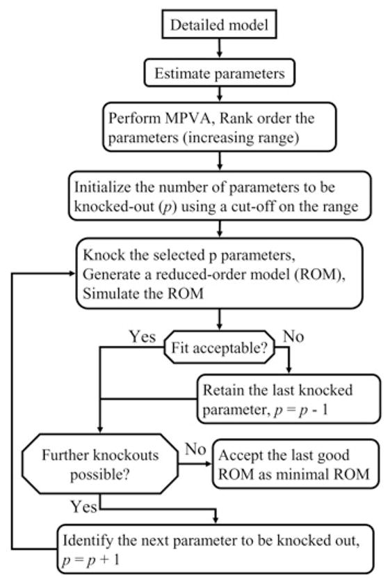
MPVA-based framework for model-reduction

3.1 Parameter estimation using hybrid GA-based pseudo-global optimisation

Model parameters are estimated between constraints by minimising the mismatch between the experimental data and the corresponding model prediction using a hybrid GA-based pseudo-global optimisation. GA is an evolutionary stochastic-search strategy [40] useful for non-linear optimisation. In the hybrid GA-based optimisation, promising candidates (see below) are identified using a GA [41–44] and then locally optimised by the Levenberg–Marquardt optimiser [45] or a sequential quadratic programming-based general non-linear optimiser [46]. These procedures (GA followed by local optimisation) result in a pool of parameter sets that fit the experimental data well. This pool consists of two parts: the parameter values generated during evolution of the population through many generations as genetic operators are applied and the parameter values obtained by local optimisation. Below, first a concise description of hybrid GA-based parameter estimation is presented and then various issues related to this method are discussed.

3.1.1 Parameter estimation

In the present GA, the parameters in the genome (the string representation) are represented through real-number notation proposed by Wolf and Moros [47]. The initial population is chosen randomly from parameters distributed uniformly on a normal-or a log-scale depending upon the specific parameter ranges. The population evolves into the next generation by transferring good candidates from the current generation (elitism [48]) and generating new members by applying crossover and/or mutation operators to parents; one parent genome is selected based on fitness and the other randomly. Thus, a fitter member is more likely to be used for crossover. The offspring genomes are evaluated by calculating the objective function (described below) and are included in the next generation. Finally, the population is sorted and members are rank-ordered according to fitness. This process is repeated for a fixed number of generations. At the end of evolution, all members of the final generation and the best members of each generation (promising candidates) undergo local optimisation as described above. Additional details on GA are provided in Section 4 of the Supplementary Material. More and exact details of hybrid GA can be found in Katare et al. [42].

3.1.2 Choice of objective function

The mismatch between the simulated and experimental data is calculated by an objective function. The objective function used in the GTPase-cycle module case study is a weighted sum of squared errors between experimental data and model predictions. This function also includes a penalty term if constraints on the parameter values are violated. Thus, there is flexibility of assigning different priorities to different constraints, allowing the user to decide the important data or features that the model must fit.

The objective function chosen affects the estimated values of the parameters. Hence, the choice of the objective function is important. For most of the applications involving development of mathematical models using experimental data (i.e. the model must fit experimental data well), the above approach of formulating an objective function works quite well. In certain applications capturing the right qualitative shape of the curve depicting the experimental data (e.g. linear increase, convex decrease, etc.) may be more important than the fit to the data. In such cases, the objective function can be appropriately modified to include an error term corresponding to the differences in the qualitative shapes/features in the experimental data and the corresponding predicted data [49]. However, at times, formulation of an appropriate objective function can be challenging. An example is the requirement of good fit to data corresponding to several scenarios (e.g. several data sets). A rule of thumb is to weigh the fit error for each data set by the inverse of the variance of the noise in the data. Thus, the acceptable fit error for data sets with lower noise would be lower as compared with that for data sets with higher noise level. With a complex objective function, it is possible that the parameter set with a lower value of the objective function may not fit the data as good as a set with slightly higher value of the objective function. To allow for such imperfections in the objective function, in the present case study, several parameter value sets whose objective value is close to the lowest fit error are regarded as good candidate parameter sets and analysed visually to select the best parameter set. After some initial trials, an error threshold was selected to automatically decide whether or not a parameter value set should be included in the pool of good sets. This error threshold is usually equal to the measurement error in experimental data or can be chosen on the basis of the variance of the noise present in experimental data. In the present case study, this information was not explicitly available.

3.1.3 Global against local optima

The issue whether local or global optima are found is relevant to all stochastic-search-based optimisation methods, including GA, Monte Carlo sampling [50], or related approaches such as differential evolution [51] and particle-swarm optimisation [52]. In these methods, there is no guarantee of finding the global optima. However, the best or some of the near-best solutions found by these methods were found to be close to global optima with respect to the position in space and the value of the objective function in many practical applications such as modelling [47, 49], protein folding [53], scheduling [54], circuit design [52] and control applications [51].

In the hybrid GA approach used here, as discussed above, the promising candidates obtained at the end of GA-based search represent promising regions in the search space. These promising candidates are further refined by local search in which depending upon how far a candidate is from its respective local minima, the candidate moves trivially (if already close) or substantially (if located far to start with). Hence, the final solutions correspond to various local minima in the search space (no guarantee that all local minima are found). Some of these local minima are actually the global minima or are quite close to the global minima [42]. Thus, a collection of near-optimal solutions is obtained, one of which is likely that global minimum. Access to a collection of near-optimal solutions is advantageous because it is possible that the solution with lowest objective function is not the best solution for the model because of measurement errors in the experimental data and difficulty in choosing appropriate (complex) objective functions.

3.1.4 Effect of error or noise in data

Experimental data always contain some measurement error or noise, which generally increases the fit error between predicted and experimental data. Other effects may also occur: Katare et al. [42] observed that several solutions with considerable difference in the values of the parameters may have similar value of the objective function, and data containing normally distributed measurement errors and/or random noise (white noise) may appear similar to error-or noise-free data (the same may be true about the values of the parameters). Hence, in cases of measurement error or noisy data, it is advisable to first raise the fit error threshold for accepting good candidate parameter sets, and then to use additional experimental data or domain-specific knowledge to differentiate between these good candidates.

3.2 Multiparametric variability analysis

Use of MPVA in model-reduction is motivated by the idea that small changes in important parameters have large impact on the system (high sensitivity with respect to these parameters), whereas even large changes in unimportant parameters have small or negligible effects (less sensitivity with respect to these parameters) [55]. In other words, even for small changes in important parameters, large changes in other (unimportant or somewhat less important) parameters would be required to bring the system to the original/desired state. Similarly, small changes in important parameters should be able to compensate for relatively much larger changes in unimportant parameters (Fig. 2).

Fig. 2. Illustration of multidimensional sensitivity analysis.

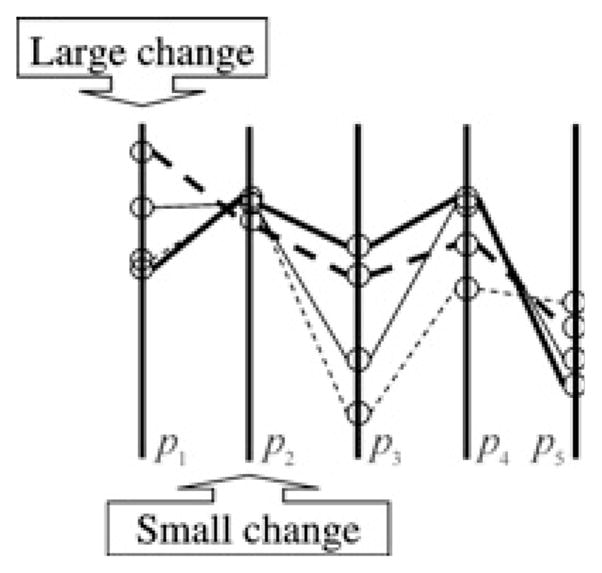
In this hypothetical example, a model contains five parameters (p₁, …, p₅), and four separate parameter value sets were found to fit experimental data. The parameter values are shown on vertical lines that represent their ranges and the specific parameter values in each parameter set are connected by lines. Parameter 2 can bear only small changes and is thus relatively important, whereas large changes can be made in parameters 1, 3, 4 and 5 and still good fit would be obtained and so these parameters are relatively less important

The notion of sensitivity proposed above is different from the traditional notion in two aspects. First, traditionally, sensitivity analysis is performed by changing one parameter at a time and measuring the effect on model output. In contrast, in our implicit MPVA method, sensitivity is characterised in terms of the overall deviations required in the parameters to minimise the deviation in the value of the objective function. This should not be confused with the dynamic analysis of sensitivity variables in a dynamic system [55]. Second, to implement our MPVA method, we use the GA-based optimisation method to search the entire parameter space and generate a pool of parameter value sets, many of which are good candidates for a pseudo-global optimal solution. No additional perturbations and simulations are needed because, due to GA-based search during optimisation, the good candidate parameter sets adequately sample the various local optima that are close to the global optima of the objective function. It can be noted that besides GA, any other stochastic-search-based optimisation such as differential evolution [51] or particle-swarm optimisation [52] can be used for MPVA.

Several good candidate parameter sets are generally available. Among these parameter sets, the fit error of the parameter set with the highest fit error is chosen as a cutoff (the error threshold introduced earlier). All parameter sets from GA and local optimisation with fit error less than or equal to this error threshold are considered to fit the data well. Their collection is called the MPVA pool. It can be noted that different parameter sets in this pool can be in different local optima regions of the parameter space and not in the unimodal region in the vicinity of the global minima. That is why this type of variability analysis is different from the well-established local sensitivity analysis. One may refer to this as global variability analysis. These sets are used as a basis to determine, for each parameter, the minimum (MIN) and maximum (MAX) values, the range (the ratio MAX/MIN) of values and the ratio of the standard deviation to the mean value. The parameters are ordered according to increasing MAX/MIN in a sorted list. The order of parameters in the sorted list is affected by several factors: (1) the amount of error or noise in the experimental data, (2) the objective function, (3) pre-specified lower and upper bounds (LB and UB) on the values of parameters in GA-based optimisation and (4) the amount of experimental data.

3.3 Generation of ROMs

3.3.1 Procedure

Parameters are knocked out either one at a time or in groups, starting with the parameter with highest MAX/MIN in the sorted list. A crucial step after each knockout is the verification of the structural integrity of the remaining model. For our purposes, this means that all chemical species except those with fixed concentration have influx and outflux reactions, allowing the system to reach steady state. If this is satisfied, the parameters of the ROM are re-optimised within their constraints by the hybrid GA-based optimisation to reflect the fact that parameter values found for the detailed model may not be optimal for the ROM. If the ROM shows satisfactory performance (i.e. fits the experimental data well or predicts the essential features), then additional parameters are knocked out. If the ROM is not acceptable, then the previous knockout is invalid, the corresponding parameter is retained and the next parameter in the sorted list is knocked out. Finding the minimal ROM can be hastened by knocking out several parameters at a time. In addition, depending upon the biological context, one may require that the values (ranges) of the parameters in the ROM should not be too different from the corresponding values (ranges) in the detailed model. The user may specify a threshold on the acceptable change in the values.

The proposed MPVA-based method emulates search along a certain branch of the search tree of the structure space and thus does not examine all possible combinations of knockouts. This can be done with integer-programming [34]. However, it is excessively complex computationally because the parameters must be re-estimated every time a new candidate ROM is tested. Thus, although the approach proposed here may not necessarily find the minimal ROM, a good ROM is generated within reasonable computing time because, in GA, the number of evaluations of the objective function, which is essentially the product of the population size and the number of generations, is nearly linear with respect to the number of unknown parameters. As knockout proceeds in a sequential manner, the total number of evaluations of the objective function is nearly quadratic with respect to the number of unknown parameters (some additional evaluations are needed because of local optimisation).

3.3.2 Discussion on the use of the methodology

To ensure that the ROMs are meaningful and they capture the essential features, it is suggested that all the experimental data and (relevant) constraints that are used to estimate the parameters for the detailed model should be used to estimate the parameters for the ROMs as well. This guideline has been used in the case study in the following section. Nevertheless, if the experimentalist wants to further restrict certain parameters (as deemed necessary because of the intended application of the ROM), then additional experimental data corresponding to scenarios/conditions in which the appropriate part of the network becomes important should be used.

The resultant ROM depends on the amount of data used for GA-based parameter estimation. As this amount is increased, some of the parameters may get restricted to narrow ranges, suggesting that such parameters are important to fit the new data. These will move up in the sorted list where they are more likely to be retained in the ROMs. Thus, the size of the smallest ROM increases (the reduction achieved decreases), although in a non-linear and discrete manner, with increasing amount of data used to estimate the parameters and to develop the ROMs. In the extreme case of using sufficient experimental data in which every parameter becomes important to satisfy some of the data, most of the parameters may get restricted assuming that GA identifies few candidates with good fit to all data sets. In this case, the sorted list will have little meaning and no model-reduction may be achieved. Hence, the information about the ultimate use of the model-reduction method and the important data/features are necessary.

Once a good ROM has been found using the proposed method, one may manually test other knockouts based upon insight about the biochemical system. These tests are biochemically informative because all relevant constraints are retained when the parameter values are re-optimised for the new model. Such synergy between computational analysis and biological insight is a powerful model reduction method that can generate novel hypotheses as discussed below in the case study of GTPase-cycle module.

3.4 Implementation

The elimination of parameters and the generation of ROMs are carried out in MATLAB [56] for simplicity of implementation. Quantitative simulation and parameter estimation are performed in C + + programming environment to achieve computational efficiency. Numerical integration and local optimisation are performed using subroutines from the International Mathematics and Statistics Library (IMSL) available from the Visual Numerics, Inc. [57].

4 Results: reduction of a detailed dynamic model of the GTPase-cycle module

In order to test our method for model-reduction, we needed a detailed model of a biochemical reaction network including its reaction rate parameters, and a data set of ‘outputs’ of that network. Although the methodology can be used to reduce (coarse-grain) the model of any biochemical system satisfying these requirements, we chose the GTPase-cycle module recently modelled in detail in our laboratory [24] based on data from the laboratory of Dr. Elliott Ross [58–61] as a test bed so that the outputs/properties of the ROMs can be easily compared and validated with those for the detailed model. Below, first, a succinct discussion on G-protein signalling and the necessary description of the detailed model of the GTPase-cycle module are presented. Then, the ROMs and other models available in the literature are discussed. In this case study, although only steady-state data are available and is used to estimate the rate parameters, the resulting ROM should be able to predict dynamic response. Hence, derivation of steady-state rate expressions, for example, using King–Altman method [5] or its variants, is not sufficient. In the following section, it is further explained why the traditional approaches for model simplification are not applicable for most of the network.

4.1 Test case study: the GTPase-cycle module

The GTPase-cycle module is a key control point in numerous cellular signalling networks. The GTPase-cycle module controls signal transduction in heterotrimeric G-protein signalling networks by regulating the activity of heterotrimeric G-proteins. In the module, G protein coupled receptors (GPCRs) activate G proteins by accelerating the exchange of GDP for GTP, and GAPs deactivate G-proteins by accelerating hydrolysis of GTP to GDP. Isolated G-proteins undergo GDP/GTP exchange and GTP hydrolysis at much slower rates. Reviews of G-protein signalling and the GTPase-cycle module have been presented by De Vries et al. [62], Gilman [63], Hall [64], Hollinger and Hepler [65], Krauss [66], Neves et al. [4] and Ross and Wilkie [67]. Several computational models have been used to investigate the effect of reaction rates, small molecule and protein concentrations, and other effects on the activity of G-proteins [68–75]. These typically invoke an accepted mechanism in which G-GDP binds agonist-bound receptor; receptor hastens exchange of GDP for GTP; G-GTP dissociates from receptor; G-GTP is hydrolysed to G-GDP either with or without a GAP; and the cycle begins anew. Recent evidence suggests an alternative mechanism in which active receptors, G-proteins and GAPs are associated in a ternary complex [60, 65, 76]. These two hypotheses reflect that, currently, at issue is how G-proteins, receptors and GAPs are organised at the plasma membrane and especially whether they form a ternary complex.

The detailed model of Bornheimer et al. [24] permits several mechanisms including the accepted mechanism described above and the ternary complex (Fig. 3) and is based on data from the mammalian GTPase-cycle module of m1 muscarinic acetylcholine receptor, Gq, and the GAP named regulator of RGS4 [58–61]. The model’s biochemical mechanism contains 17 chemical species and 24 reversible reactions and was mathematically implemented with 17 ODEs and 48 reaction rate parameters. Seven of the parameters were directly measured and another 41 were constrained between UBs and LBs evident from experimental data; of these, 28 were optimised and 13 were calculated to maintain material equilibrium using the GA-based parameter estimation procedure presented in the previous section. The experimental data used, the specific constraints on parameters, and the objective function are described in the Supplementary Material (Tables 2 and 3 and Sections 1–4 in the Supplementary Material). The main simplifications of the biochemical mechanism of the detailed model are that (a) all receptor is considered active (changing its concentration mimics change in agonist binding to receptor), (b) the G_βγ subunit is not modelled and (c) perfect mixing is assumed, meaning that diffusion effects and spatial variations are not considered; these simplifications are retained in all ROMs described below. The important outputs of the model are the fraction of active G-protein (Z), and GTP turnover rate (v) [24]. The expressions for Z and v (at steady state) are

Fig. 3. Reaction network for the detailed model of the GTPase-cycle module [24].

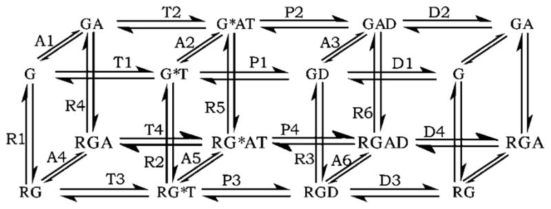
G: G-protein, R: agonist-bound GPCR, A: GAP, T: GTP, D: GDP. G-proteins bind T, hydrolyse it to D and D dissociates; in each state, G-proteins reversibly bind R (which accelerates GDP/GTP exchange) or GAP (which accelerates GTP hydrolysis). G* denotes the active form of G-protein. Free GTP, GDP and phosphate (P_i) are not shown for simplicity. Each reaction is labelled with its name, where A_i (i = 1, 2, 3, etc.) denotes exchange (association or dissociation) of GAP, R_i denotes exchange of GPCR, T_i denotes exchange of GTP, P_i denotes exchange of a phosphate and D_i denotes exchange of GDP

$$\begin{array}{l}Z=\frac{[\text{GT}]+[\text{RGT}]+[\text{RGAT}]+[\text{GAT}]}{{[\text{G}]}_{\text{total}}}\\ v=\frac{\text{P}-4^{\ast }[\text{RGAT}]+\text{P}-2^{\ast }[\text{GAT}]+\text{P}-3^{\ast }[\text{RGT}]+\text{P}-1^{\ast }[\text{GT}]}{{[\text{G}]}_{\text{total}}}\end{array}$$ (1)

where [G]_total is the sum of the concentrations of all species involving G-protein. The ‘+’ or ‘−’ sign in the parameter names (e.g. in P − 4) indicate that the corresponding reaction is an association or dissociation reaction, respectively (Section 1 of Supplementary Material). The identifier ‘*’ from G*T, RG*T and so on has been removed for simplicity. Z is dimensionless. v is expressed as (mol P_i/s)/mol G (i.e. moles of phosphate produced or GTP hydrolysed per second per mole of G-protein present in the system) and hence its overall dimension is s⁻¹.

In the study of the detailed model [24], the outputs Z and v were calculated over a wide range of concentrations of R and GAP. This revealed four limiting signalling regimes (LSRs): G, RG, RGA, and GA. In each, receptor and/or GAP are either saturating or absent, GTP, GDP, and P_i (phosphate) are set at cellular concentrations (468 μM, 149 μM and 4.4 mM, respectively [77]; [GD] is initialised to 10.0 nM) and characteristic values of Z and v result. In limiting signalling regime G, receptor and GAP are absent, Z = 0.0076 and v = 9.9 × 10⁻⁵ s⁻¹; in RG, receptor is saturating, GAP is absent, Z = 0.98 and v = 0.012 s⁻¹; in RGA, both receptor and GAP are saturating, Z = 0.096 and v = 2.4 s⁻¹; in GA, GAP is saturating, receptor is absent, Z = 4.6 × 10⁻⁵ and v = 0.0012 s⁻¹. Mechanistically, these limiting signalling regimes arise by dominance of one of the four kinetic paths forming horizontal edges of the mechanism shown in Fig. 3 (e.g. G → GT → GD → G). These paths were called extreme paths. In the results described below, the ROMs are judged in part for their ability to qualitatively produce the limiting signalling regimes at cellular nucleotide concentrations.

The traditional methods of model simplification based on assumptions of equilibrium of reversible reactions and quasi-steady-state assumption on enzyme–substrate complexes are not applicable for the GTPase-cycle system. To verify this, a detailed comparative analysis of the species concentration during transients was carried out across a wide range of the concentration of the receptor and GAP covering the four LSRs (Section 5 and Fig. 10 in the Supplementary Material). It was found that the equilibrium holds true only for the reactions D2–D4. For other reactions, including D1, A1–A6 and R1–R6, neither linearity nor Michaelis–Menten-like dependence is observed. Thus, the traditional approaches of model simplification do result in some simplification, but for most of the network they are not applicable during the initial transients which are considered important for cellular signalling. This is not surprising as Bornheimer et al. [24] have shown the existence of two distinct regimes (mass action regime and stoichiometric regime). It is true that the approach proposed in this article and the traditional approaches can be used synergistically to achieve more simplification/reduction as compared with the simplification achieved by one approach alone.

To develop ROMs of the GTPase-cycle module that fits the experimental data, the method described in the previous section is used. The sorted list of parameters according to increasing range is given in Table 1 (additional details provided in Table 4 in Supplementary Material). ROMs are generated by eliminating reactions starting from the end in this list, that is, D+1 is eliminated first, then R−1 and so on. All the data and (relevant) thermodynamic constraints that were used with the detailed model are also used to estimate the parameters for all the ROMs. For each ROM discussed below, the value of parameters corresponding to the best set from GA-based estimation and the MAX and MIN values and its comparison with the MAX and MIN for the base (detailed) model are provided in the Supplementary Material (Section 5).

Table 1.

List of all parameters of the detailed model sorted according to increasing range (MAX/MIN)

Sr. No. in sorted list	Parameter name
1–5	D − 3, P − 2, P − 1, P − 3, P − 4
6–10	D − 1, D − 2, R + 3, T + 3, A + 2
11–15	D − 4, A − 5, A + 5, A − 2, T − 2
16–20	T + 1, R + 5, T + 4, A − 3, T − 4
21–25	R − 5, R + 4, R + 6, A + 3, D + 3
26–30	R − 2, A + 6, A + 4, R − 6, A + 1
31–35	R + 2, A − 6, P + 3, T − 3, T + 2
36–40	T − 1, D + 2, D + 4, R + 1, R − 3
41–45	P + 4, P + 1, P + 2, R − 4, A − 4
46–48	A − 1, R − 1, D + 1

MAX and MIN are calculated over the MPVA pool (Table 4 in Supplementary Material). The parameters with little or no variation (small MAX/MIN), such as D − 3, R + 3 and so on are in the top rows. The parameters with large variations (large MAX/MIN), such as D + 1, P + 4 and so on are in the bottom rows.

4.2 The ROMs developed using the MPVA-based framework

4.2.1 Automatically generated ROM 1

The method outlined in the previous section automatically eliminated the following 27 reactions resulting in the biochemical mechanism depicted in Fig. 4a: D + 1, R − 1, A − 1, A − 4, R − 4, P + 2, P + 1, P + 4, R − 3, R + 1, D + 4, D + 2, T − 1, T + 2, T − 3, P + 3, A − 6, R + 2, A + 1, R − 6, A + 4, A + 6, D + 3, A + 3, R + 6, R − 5, T − 4. Most are the reverse of canonical GTPase-cycle reactions such as GTP association, GTP hydrolysis, GDP dissociation and association of R and dissociation of GAP from G-GDP species. Knockout of these reactions does not violate the bulk of data on the function of the GTPase-cycle and is in keeping with simpler models of the GTPase-cycle (e.g. [60, 66–68, 72]), thereby indicating the fidelity of the method in retaining key mechanisms during model-reduction.

Fig. 4. ROM with 21 parameters (27 parameters have been eliminated).

a Reaction network (the eliminated reactions are shown with grey arrows). Three of the extreme (horizontal) pathways – G, RG, and RGA – are retained. In path GA, instead of the forward reaction from GA to G*AT, the reverse reaction from G*AT to GA is retained

b Fit of the simulated data to experimental data: plot 1: low [GAP] and varying [GTP]; plot 2: no GAP and varying GTP; plot 3: high [GTP] and varying [GAP]

Simulations of experiments were performed as described in the Supplementary Material. The data predicted by the detailed model (base model) are also shown. The horizontal dashed line corresponds to half-maximum v. The dimension of v is mol/s of P_i per mol of G. For simplicity, it is indicated as s⁻¹

c Predicted Z (fraction of active G-protein) for varying [A] and [R]. The four LSRs are shown

d Comparison of the ranges (MAX/MIN) for various parameters in the ROM with the ranges of the corresponding parameters in the detailed model. The LB and UB used for optimisation and the value of the parameters corresponding to the best-fit are also shown. The ‘+’ and ‘−’ signs in the parameter names denote association and dissociation reactions, respectively (e.g. P − 1 is the rate constant for the hydrolysis of G*T (dissociation of P_i))

Text style for the parameter names: fixed parameters, bold-face; optimised parameters, regular font-weight

This ROM fitted the experimental data well and reproduced three of the four LSRs (Figs. 4b and 4c). Fig. 4b shows the fit of predicted data to the experimental data. The three data sets listed in Table 2 (Supplementary Material) are shown in the three plots. The fit of the predictions of the detailed model is also shown. The experimental conditions for the data sets shown in the three plots are: plot 1: low [GAP] and varying [GTP]; plot 2: no GAP and varying GTP; plot 3: high [GTP] and varying [GAP]. The LSR GA is captured partially (Fig. 4c); saturating [GAP] appears to be higher than the corresponding saturation level in the detailed model. Notably, this ROM retained all ternary complexes of G-protein with R and GAP.

Most parameter values were confined within less than one order of magnitude as determined by sensitivity analysis (Fig. 4d, and Table 5 of Supplementary Material), indicating a relatively well-constrained ROM. There were, however, some widely varying parameters. The comparison shown in Fig. 4d reveals the following interesting facts:

1. Wider parameter ranges in the ROM: Although many parameter ranges in the ROM are narrow, there are several, such as A − 3, T + 1, T − 2 and R + 4, which span 2–3 orders of magnitude. This is because some of the eliminated reactions were involved in thermodynamic cycles, and hence the corresponding thermodynamic constraints are no longer applicable. Thus, the parameter space became less restrictive. Still, all parameter ranges satisfy relevant constraints.

2. Difference in parameter ranges for the detailed model and the ROM: Based upon comparison of parameter ranges in the detailed model and ROM, we define four categories of parameters: (1) fixed parameters (D − 3, P − 2, etc.), (2) those for which the range in the ROM contains the range in the detailed model or vice versa (A − 2, A − 3, T − 2, etc.), (3) those for which the ranges partially overlap (A + 5) and (4) those with non-overlapping ranges (R + 5, R + 4). The fourth category is most surprising: it indicates that if one were to require that the parameters in the ROM be restricted to the range for the parameters in the detailed model (for the good sets), then for the current reaction network no parameter values with satisfactory fit would have been found. There is, however, no need to apply such a restriction because the true values of the parameters could possibly lie outside their range for the detailed model. It is noted that the detailed model is also an approximation of the real biochemical system.

Regardless of the variation in parameters, all parameters satisfy known constraints. If this were not the case, or if sufficient constraints were unavailable, then the values of some of parameters of the ROM may exceed the limits observed in experimental systems. On this note, in two cases – R + 4 and R + 5 – the maximum rate of the association reaction met or slightly exceeded the diffusion limit (<10⁹ M⁻¹ s⁻¹). In these cases, the maximum rate was set at 10¹⁰ M⁻¹ s⁻¹ to compensate for uncertainties in the measurement of receptor concentration; however, the rates determined by optimisation were still reasonable (R + 4 = 3.96 × 10⁹ M⁻¹ s⁻¹ and R + 5 = 5.06 × 10⁸ M⁻¹ s⁻¹) (Fig. 4d, and Table 5 in Supplementary Material). If the theoretical limits must be imposed, then these constraints can be imposed explicitly.

4.2.2 Automatically generated ROM 2

Next, the method attempted to eliminate an additional eight parameters based on their order in the sorted list, failing in four cases (A − 3, T + 4, T + 1, A + 5) and succeeding in four cases (R + 5, T − 2, A − 2, A − 5). This shows that some parameters were important despite a position in the sorted list above other parameters that could be knocked out. Knockout of R + 5, T − 2, A − 2 and A − 5 does not violate the bulk of data on the function of the GTPase-cycle. Retention of A − 3, T + 4, T+1 and A+5 is in agreement with the data that GAP binds G-GTP species and dissociates from G-GDP species, and that GTP binds empty G-protein species; however, retention of T+4 also implies that RGA exists although there is little empirical evidence for it [78].

The resulting ROM is the minimal ROM that was generated automatically, containing 17 parameters (Fig. 5a). It fits the experimental data well in most cases (Fig. 5b) and produces three of the four LSRs well and LSR GA partially (Fig. 5c). The experimental data on GTPase rate during GAP titration (plot 3 in Fig. 5b) fits imperfectly. For this ROM too, the general features of the ranges of the parameters with good fit are similar to those shown in Fig. 4d (see Table 6 and Fig. 11 in the online supplementary material); hence, they are not discussed explicitly.

Fig. 5. Minimal ROM obtained using the MPVA-based automated approach has 17 parameters.

a Reaction network. This ROM has four less reactions (R + 5, T − 2, A − 2, A − 5) as compared with the ROM of Fig. 4a. Three of the extreme pathways – R, RG and RGA – are retained; in path GA, reaction T2 is absent

b Fit of the data predicted by the ROM to experimental data

c Four LSRs are predicted

4.3 Inability of the published models to fit the experimental data and capture key predictions of the detailed model

Starting with an early model of the GTPase-cycle module proposed by Cassel et al. [68], as more experimental data became available, several other models with additional details were published [60, 66, 67, 72]; these models each have fewer interactions than in the detailed model of Bornheimer et al. [24]. In terms of complexity (number of parameters), these models are comparable in size to the 17-parameter ROM developed using the MPVA-based method. Hence, we examined two of these models – a current textbook model [66] and a hypothetical, more sophisticated model of Biddlecome et al. [60] – by simulating them computationally (including parameter estimation) to test their ability to fit the experimental data and predict the four LSRs. The experimental data and the methodology used for parameter estimation for these models are exactly the same as for the detailed model and the MPVA-based ROMs.

The textbook model (Fig. 6a) includes the GTPase-cycle of isolated G-proteins, the GEF (guanine nucleotide (GDP/GTP) exchange factor) activity of the active receptor, and the GTPase activity of GAP, and consists of 12 parameters and 13 ODEs. Unlike the 17-parameter ROM, it excludes the ternary complex of G-protein with active receptor and GAP. The textbook model does not fit the experimental data well (Fig. 6b). For instance, when GAP is saturating only 25% of the experimentally observed turnover rate is attained, suggesting that RGA, RG*AT and RGAD are required. However, this model does capture the LSRs G, RG, GA and RGA well (Fig. 12a in the online supplementary material); the last is surprising given that extreme pathway RGA is not modelled. A putative explanation is that the presence of parts of the extreme pathways RG and GA compensates for the absence of the extreme pathway RGA. Results of sensitivity analysis are listed in Table 7 and are shown in Fig. 12b of the online supplementary material.

Fig. 6. Textbook model [66].

a Reaction network. The extreme pathway RGA is not included and the pathways GA and RG are partially included

b Fit of the predicted data to experimental data

A mechanistic explanation for poor fit to data sets 1 and 3 (plots 1 and 3, respectively, in Fig. 6b) and good fit to data set 2 (plot 2) is as follows. In the data for plot 2, no GAP (A) is present. Hence, the presence or absence of the reactions in which GAP associates has no effect and fit to plot 2 is good. Alternatively, in the data for plots for 1 and 3, both GAP and receptor are present. Hence, the reactions involving association of receptor and GAP become important. As the model excludes the ternary complex RGAT and the reaction P − 4 (hydrolysis of RGAT), which accounts for substantial flux in the biochemical system (P − 4 = 25 s⁻¹), the model is able to capture only part of the full GTP turnover rate. As P − 2 = P − 4 and that the reaction corresponding to P − 2 is included in the model, a crude analysis validates the above observation assuming that, in the real biochemical system, steady-state concentration of RGAT is about twice as that of GAT.

An alternative model was published by Biddlecome et al. [60] that includes the ternary complex of G-protein with active receptor and GAP (Fig. 7a) but excludes extreme pathway GA. This model consists of 12 parameters and 14 ODEs. The fit to experimental data is impressive (Fig. 7b) for a relatively small model, suggesting that the ternary complex plays a key role. Additionally, the LSRs G, RG and RGA are captured well (Fig. 13a in the online supplementary material). LSR GA does not exist because extreme pathway GA is not included in this model; put another way, at very low receptor concentration (10⁻¹⁵ M), there is no change in Z for variation in [GAP]. Results of sensitivity analysis are listed in Table 8 and shown in Fig. 13b of the online supplementary material.

Fig. 7. Biddlecome et al. [60] model.

a Reaction network for a 12-parameter model [60, 67]

b Predictions made by the 12-parameter model (continuous curve) and the predictions made by a smaller ROM with 10 parameters that is derived by eliminating the parameters T + 4 and D − 4 (dashed curve)

The ROM consisting of 17 reactions that were generated using the MPVA-based automated method combines the best qualities of the textbook model and Biddlecome et al. [60] model in capturing the experimental data (textbook model fails) as well as the four LSRs (the Biddlecome et al. [60] model fails). Thus, in a semi-quantitative way, one can say that structural superposition leads to superposition of the model predictions. More importantly, the automated method arrived at a reasonable ROM that integrated and expanded upon key proposed models from the literature although it was not biased towards them.

4.4 Importance of the ternary complex of active m1 MAchR – Gq*-GTP – RGS4

To further identify the relative importance of RGA, RGAD and RG*AT in the Biddlecome et al. [60] model, we manually knocked out the inactive complex RGA and the reactions T + 4 and D − 4 from the Biddlecome et al. [60] model so that the RG*AT complex – which stimulates fast GTP hydrolysis – must re-associate with each turn of the GTPase-cycle. This resulted in a new ROM of 10 parameters and 13 ODEs (not shown). This model fit the data relatively well (Fig. 7b, thin-dashed curve), capturing more than 75% of maximum v in all data sets. Thus, RG*AT is extremely important and capable of partially rescuing the fit to data (compare with Fig. 6) even if it must re-associate with each turn of the GTPase-cycle. However, this ROM does not reproduce LSR GA (because extreme pathway GA is completely knocked out) and is unlikely to fit data involving only G-protein and GAP, suggesting that it is overly simplified (Fig. 13c in the online supplementary material). The results of sensitivity analysis for the 10-parameter ROM are listed in Table 8 and are shown in Fig. 13d in the online supplementary material. It was hypothesised that retaining parts of the pathway GA by including the reactions A + 2, P − 2 and A − 3 might capture LSR GA. Indeed, when these three reactions are included in the Biddlecome et al. [60] model, an ROM of 15 parameters (Fig. 8a) and 16 ODEs is formed that fits the experimental data well (Fig. 8b) and captures all four LSRs (Fig. 8c). This ROM is the absolute minimal ROM. The results of sensitivity analysis for the 10-parameter ROM are listed in Table 9 and are shown in Fig. 14 in the online supplementary material. The predictions of this 15-parameter ROM are only slightly better than the 17-parameter ROM generated automatically (Fig. 5) demonstrating the strength of the MPVA-based reduced-order modelling.

Fig. 8. 15-parameter model obtained by adding reactions A + 2, P − 2 and A−3 to the 12-parameter model proposed by Biddlecome et al. [60].

With this modification, the LSR GA is also captured

a Reaction network

b Fit to the experimental data

c Prediction of the four LSRs

To finally demonstrate whether the ternary complex of G-protein with active receptor and GAP is required, only RG*AT and hence, the associated eight parameters T4, P4, A5 and R5, were eliminated from the detailed model. This ROM consists of 40 parameters and 16 ODEs (Fig. 9a). Similar to the textbook model (Fig. 6), this model does not fit the data well (Fig. 9b; the LSRs G, RG and GA exist (data not shown); results of sensitivity analysis listed in Table 10 and shown in Fig. 15 of the online supplementary material). For example, only ~25% of the maximum turnover rate is attained in data sets 1 and 3. This complements the previous result that RG*AT – even if it must re-associate with each turn of the GTPase-cycle – is required for the GTPase-cycle to reach ~75% of maximum v. Furthermore, it demonstrates the necessity of retaining RG*AT (and at least one association reaction for influx to RG*AT and one dissociation reaction for outflux from RG*AT) to fit the experimental data.

Fig. 9. 40-parameter model in which RG*AT and eight associated parameters are eliminated.

a Reaction network

b Poor fit in plots 1 and 3 indicates that RG*AT must be included in the model

5 Discussion

Restricting the size of computational models is a major problem in systems biology. We devised a method to solve this problem and tested it on a detailed model of the GTPase-cycle, leading to the key mechanistic insight that the ternary complex of G-protein with receptor and GAP is required. As stated in Section 4.1, the proposed approach is needed for the GTPase system because the traditional approaches are not applicable for a large part of the network during transients. Below we will discuss separately the applicability and advantages of the algorithm and the importance of the ternary complex.

5.1 Utility/novelty of the MPVA-based approach

The MPVA-based approach provides a novel and intuitively simple, yet powerful quantitative framework for model-reduction. The notion of MPVA used in this work is particularly suitable for the analysis of biological systems. The computational complexity of the methodology scales well with increase in the size of the model and hence is suitable for constraining biological systems for which a detailed model could run into thousands of equations and parameters. Three important aspects of the approach are: (1) the ability to deal with parameters whose exact values are unknown but constrained between certain bounds and the ability to incorporate physiologically relevant and critical mechanistic information in the form of suitable constraints, (2) for a single ROM, the availability of a pool of good candidate parameter sets to choose from, and (3) the availability of several alternate ROMs at the end of the procedure. These aspects help deal with uncertainty in both the experimental data and the accuracy of the initial biochemical reaction scheme. For instance, the alternate ROMs may fit specific experimental data for which very simple ROMs fail. Additionally, new experimental data are continuously generated and therefore model update is necessary [79]. Maurya et al. [35] proposed three types of model update: (1) update of the parameters by re-optimisation, (2) update of the flux expressions, and (3) update of the network structure. Notably, types 1 and 3 are included in our MPVA-based approach for model-reduction. Thus, the methodology proposed here is suitable for developing ROMs for the modules in biological systems. The MPVA approach can be used for a network of modules too but the elimination achieved on the inter-module reactions would be low because of the complex effects of feedback and feed-forward mechanisms among the modules.

As already discussed in Section 3, the amount of experimental data used – for both constraining parameters within bounds and fitting during parameter estimation –and its quality (reflected as the amount of noise in data and the coverage of various physiological conditions which the model should be able to capture) strongly affect the ROM developed. Similarly, aspects of the computational method, especially the design of the objective function and interpretation of objective values, can also affect the results but not so much as the amount of data itself.

5.2 Required ternary complex of receptor, G-protein and GAP

The collision coupling model is the traditional qualitative model of the early steps in G-proteins signalling and posits that inactive G-proteins associate with active receptors that stimulate GDP/GTP exchange, then dissociate as active G-proteins to stimulate downstream signalling pathways via specific effector proteins [73, 80–82]. Our ROMs suggest instead that G-proteins must interact at once with receptor and GAP in a ternary complex in which G-proteins are rapidly turned on and off by receptors and GAPs. In this model, it is likely that effectors and other protein interaction partners of G-proteins are co-localised with the ternary complex, perhaps in larger signalling complexes. We specifically predict that the ternary complex forms in the module comprising Gq, active m1 MAchR and RGS4 and suggest that it may form in other GTPase-cycle modules.

Several other lines of evidence suggest the formation of a ternary complex. Recently it was found that RGS2 and RGS4 bind the third intercellular loop of m1 MAchR independent of G-proteins and that for RGS2 this interaction is maintained in the presence of Gq (RGS4 not examined) [78]. The N-terminus of RGS4 potentiated RGS4 GAP activity in m1 MAchR – Gq vesicles, suggesting a role in targeting the RGS4 to the receptors or G proteins [83]. Biddlecome et al. [60] proposed a mechanism that can be called kinetic scaffolding in which m1 MAchR and RGS4 are assumed not to interact, but the GAP activity of RGS4 on RG*AT is rapid enough to outcompete dissociation of the receptor–G*GTP complex, yielding a functional ternary complex. Recently, Benians et al. [76, 84] showed, using fluorescence resonance energy transfer microscopy, that a stable physical interaction occurs between RGS8–yellow fluorescent protein and G_oα_A – cyan fluorescent protein in the presence and absence of receptor activation in human embryonic kidney 293 cells.

The definition of RGA, RG*AT and RGAD in our model does not specify whether the complex is maintained by a physical interaction or kinetic scaffolding mechanism. Hence, the proposed reaction network represents both types of interaction. However, it does exclude the possibility of an additional scaffolding protein because only the proteins Gq, m1 MAchR and RGS4 were included in the experimental studies that generated the data used for our models.

Ternary complexes of G-protein, receptor and GAP may occur in many GTPase-cycle modules. In the analysis of the detailed model [24], it was concluded that extreme pathway RGA is specialised for rapid signal modulation with substantial G-protein activity. Therefore, this type of signalling is expected to extend beyond the muscarinic family of receptors to other signalling pathways requiring rapid signal attenuation, such as other receptors that regulate ion channels, rhodopsin in the phototransduction cascade and receptors involved in neuronal processes. However, in these cases additional molecules may be involved to maintain or regulate GTPase-cycle module signalling complexes as is the case in the phototransduction cascade [85].

Computational modelling is of increasing importance to biology as the size and detail of data sets increases. Of equal importance is containing the size and complexity of the computational models without losing fidelity. We have presented a method for reducing biological models comprised of many parameters (where the value of each parameter need not be known) and applied it to reduce a detailed model of the GTPase-cycle module. An implicit MPVA is used to guide the model-reduction process. The MPVA is performed using the results of a hybrid GA-based optimisation of the detailed model itself and, hence, no additional perturbation simulations are required. The methodology is suitable to deal with uncertainty in the values of model parameters and its complexity scales well with the model size. Most importantly, the model-reduction framework allows for the inclusion of constraints that are of physiological and biochemical relevance. The model-reduction method presented here can be applied to reduce any computational model of a biochemical system, regardless of its size and complexity. Further, the proposed approach can be used with the traditional approaches synergistically to achieve more simplification/reduction as compared with the simplification achieved by one approach alone.

References

- 1.Asthagiri AR, Lauffenburger DA. A computational study of feedback effects on signal dynamics in a mitogen-activated protein kinase (MAPK) pathway model. Biotechnol Progr. 2001;17(2):227–239. doi: 10.1021/bp010009k. [DOI] [PubMed] [Google Scholar]
- 2.Bhalla US, Iyengar R. Emergent properties of networks of biological signaling pathways. Science. 1999;283(5400):381–387. doi: 10.1126/science.283.5400.381. [DOI] [PubMed] [Google Scholar]
- 3.Weng GZ, Bhalla US, Iyengar R. Complexity in biological signaling systems. Science. 1999;284(5411):92–96. doi: 10.1126/science.284.5411.92. [DOI] [PMC free article] [PubMed] [Google Scholar]
- 4.Neves SR, Ram PT, Iyengar R. G protein pathways. Science. 2002;296(5573):1636–1639. doi: 10.1126/science.1071550. [DOI] [PubMed] [Google Scholar]
- 5.King EL, Altman C. A schematic method of deriving the rate laws for enzyme-catalyzed reactions. J Phys Chem. 1956;60(10):1375–1378. [Google Scholar]
- 6.Li YX, Rinzel J. Equations for Insp(3) receptor-mediated [Ca2+](I) oscillations derived from a detailed kinetic model – a Hodgkin–Huxley-like formalism. J Theor Biol. 1994;166(4):461–473. doi: 10.1006/jtbi.1994.1041. [DOI] [PubMed] [Google Scholar]
- 7.Weiss JM, Morgan PH, Lutz MW, Kenakin TP. The cubic ternary complex receptor-occupancy model. 1: Model description. J Theor Biol. 1996;178(2):151–167. doi: 10.1006/jtbi.1996.0139. [DOI] [PubMed] [Google Scholar]
- 8.Bhalla US, Ram PT, Iyengar R. MAP kinase phosphatase as a locus of flexibility in a mitogen-activated protein kinase signaling network. Science. 2002;297(5583):1018–1023. doi: 10.1126/science.1068873. [DOI] [PubMed] [Google Scholar]
- 9.Mishra J, Bhalla US. Simulations of inositol phosphate metabolism and its interaction with InsP(3)-mediated calcium release. Biophys J. 2002;83(3):1298–1316. doi: 10.1016/S0006-3495(02)73901-5. [DOI] [PMC free article] [PubMed] [Google Scholar]
- 10.Bhalla US. Signaling in small subcellular volumes. I. Stochastic and diffusion effects on individual pathways. Biophys J. 2004;87(2):733–744. doi: 10.1529/biophysj.104.040469. [DOI] [PMC free article] [PubMed] [Google Scholar]
- 11.Brinkerhoff CJ, Woolf PJ, Linderman JJ. Monte Carlo simulations of receptor dynamics: insights into cell signaling. J Mol Histol. 2004;35(7):667–677. doi: 10.1007/s10735-004-2663-y. [DOI] [PubMed] [Google Scholar]
- 12.Ashburner M, Ball CA, Blake JA, Botstein D, Butler H, Cherry JM, Davis AP, Dolinski K, Dwight SS, Eppig JT, Harris MA, Hill DP, Issel-Tarver L, Kasarskis A, Lewis S, Matese JC, Richardson JE, Ringwald M, Rubin GM, Sherlock G. Gene ontology: tool for the unification of biology. Nat Genet. 2000;25(1):25–29. doi: 10.1038/75556. [DOI] [PMC free article] [PubMed] [Google Scholar]
- 13.Asthagiri AR, Lauffenburger DA. Bioengineering models of cell signaling. Annu Rev Biomed Eng. 2000;2:31–53. doi: 10.1146/annurev.bioeng.2.1.31. [DOI] [PubMed] [Google Scholar]
- 14.Hartwell LH, Hopfield JJ, Leibler S, Murray AW. From molecular to modular cell biology. Nature. 1999;402(6761):C47–C52. doi: 10.1038/35011540. [DOI] [PubMed] [Google Scholar]
- 15.Hofestadt R, Thelen S. Quantitative modeling of biochemical networks. Silico Biol. 1998;1:39–53. [PubMed] [Google Scholar]
- 16.Lauffenburger DA. Cell signaling pathways as control modules: complexity for simplicity? Proc Natl Acad Sci USA. 2000;97(10):5031–5033. doi: 10.1073/pnas.97.10.5031. [DOI] [PMC free article] [PubMed] [Google Scholar]
- 17.Neves SR, Iyengar R. Modeling of signaling networks. Bioessays. 2002;24(12):1110–1117. doi: 10.1002/bies.1154. [DOI] [PubMed] [Google Scholar]
- 18.Ravasz E, Somera AL, Mongru DA, Oltvai ZN, Barbasi AL. Hierarchical organization of modularity in metabolic networks. Science. 2002;297(5586):1551–1555. doi: 10.1126/science.1073374. [DOI] [PubMed] [Google Scholar]
- 19.Rumbaugh J, Blaha M, Premerlani W, Eddy F, Lorenson W. Object oriented modeling and design. Prentice-Hall; Englewood Cliffs, NJ: 1991. [Google Scholar]
- 20.Hoffmann A, Levchenko A, Scott ML, Baltimore D. The I kappa B–NF–kappa B signaling module: temporal control and selective gene activation. Science. 2002;298(5596):1241–1245. doi: 10.1126/science.1071914. [DOI] [PubMed] [Google Scholar]
- 21.Saucerman JJ, Brunton LL, Michailova AP, McCulloch AD. Modeling beta-adrenergic control of cardiac myocyte contractility in silico. J Biol Chem. 2003;278(48):47997–48003. doi: 10.1074/jbc.M308362200. [DOI] [PubMed] [Google Scholar]
- 22.Cideciyan AV, Jacobson SG. An alternative phototransduction model for human rod and cone ERG a-waves: normal parameters and variation with age. Vis Res. 1996;36(16):2609–2621. doi: 10.1016/0042-6989(95)00327-4. [DOI] [PubMed] [Google Scholar]
- 23.Lamb TD, Pugh EN. A quantitative account of the activation steps involved in phototransduction in amphibian photoreceptors. J Physiol London. 1992;449:719–758. doi: 10.1113/jphysiol.1992.sp019111. [DOI] [PMC free article] [PubMed] [Google Scholar]
- 24.Bornheimer SJ, Maurya MR, Farquhar MG, Subramaniam S. Computational modeling reveals how interplay between components of a GTPase-cycle module regulates signal transduction. Proc Natl Acad Sci USA. 2004;101(45):15899–15904. doi: 10.1073/pnas.0407009101. [DOI] [PMC free article] [PubMed] [Google Scholar]
- 25.Conzelmann H, Saez-Rodriguez J, Sauter T, Bullinger E, Allgower F, Gilles ED. Reduction of mathematical models of signal transduction networks: simulation-based approach applied to EGF receptor signaling. Syst Biol. 2004;1(1):159–169. doi: 10.1049/sb:20045011. [DOI] [PubMed] [Google Scholar]
- 26.Green M, Limebeer DJN. Linear robust control. Prentice-Hall; 1995. [Google Scholar]
- 27.Petzold L, Zhu WJ. Model reduction for chemical kinetics: an optimization approach. AIChE J. 1999;45(4):869–886. [Google Scholar]
- 28.Vora N, Daoutidis P. Nonlinear model reduction of chemical reaction systems. AIChE J. 2001;47(10):2320–2332. [Google Scholar]
- 29.Tikhonov AN. Systems of differential equations containing a small parameter in the derivatives. Mat Sbornik. 1952;31(73):575–586. [Google Scholar]
- 30.Stephanopoulos G, Aristidou A, Nielsen J. Metabolic engineering: principles and methodologies. Academic Press; San Diego, USA: 1998. Review of cellular metabolism; pp. 21–79. [Google Scholar]
- 31.Edwards K, Edgar TF, Manousiouthakis VI. Kinetic model reduction using genetic algorithms. Comput Chem Eng. 1998;22(1–2):239–246. [Google Scholar]
- 32.Okino MS, Mavrovouniotis ML. Simplification of mathematical models of chemical reaction systems. Chem Rev. 1998;98(2):391–408. doi: 10.1021/cr950223l. [DOI] [PubMed] [Google Scholar]
- 33.Androulakis IP. Kinetic mechanism reduction based on an integer programming approach. AIChE J. 2000;46(2):361–371. [Google Scholar]
- 34.Bhattacharjee B, Schwer DA, Barton PI, Green WH. Optimally reduced kinetic models: reaction elimination in large-scale kinetic mechanisms. Combust Flame. 2003;135(3):191–208. [Google Scholar]
- 35.Maurya MR, Katare S, Patkar PR, Rundell A, Venkatasubramanian V. A systematic framework for the design of reduced-order models for signal transduction pathways from a control theoretic perspective. Comput Chem Eng. 2005 in print. [Google Scholar]
- 36.Blower SM, Dowlatabadi H. Sensitivity and uncertainty analysis of complex models of disease transmission – an HIV model, as an example. Int Stat Rev. 1994;62(2):229–243. [Google Scholar]
- 37.McKay MD, Beckman RJ, Conover WJ. A comparison of three methods for selecting values of input variables in the analysis of output from a computer code. Technometrics. 1979;21(2):239–245. [Google Scholar]
- 38.Zi Z, Cho K, Sung M, Xia X, Zheng J, Sun Z. In silico identification of the key components and steps in IFN-γ induced JAK-STAT signaling pathway. FEBS Lett. 2005;579(5):1101–1108. doi: 10.1016/j.febslet.2005.01.009. [DOI] [PubMed] [Google Scholar]
- 39.Takahashi RHC, Ramirez JA, Vasconcelos JA, Saldanha RR. Sensitivity analysis for optimization problems solved by stochastic methods. IEEE Trans Magn. 2001;37(5):3566–3569. [Google Scholar]
- 40.Goldberg DE. Genetic algorithms in search, optimization and machine learning. Addison-Wesley; Reading, MA: 1989. [Google Scholar]
- 41.Androulakis IP, Venkatasubramanian V. A genetic algorithmic framework for process design and optimization. Comput Chem Eng. 1991;15(4):217–228. [Google Scholar]
- 42.Katare S, Bhan A, Caruthers JM, Delgass WN, Venkatasubramanian V. A hybrid genetic algorithm for efficient parameter estimation of large kinetic models. Comput Chem Eng. 2004;28(12):2569–2581. [Google Scholar]
- 43.Sundaram A, Venkatasubramanian V. Parametric sensitivity and search space characterization studies of genetic algorithms for computer-aided polymer design. J Chem Inform Comput Sci. 1998;38(6):1177–1191. [Google Scholar]
- 44.Venkatasubramanian V, Chan K, Caruthers JM. Evolutionary design of molecules with desired properties using the genetic algorithm. J Chem Inform Comput Sci. 1995;35(2):188–195. [Google Scholar]
- 45.Marquardt DW. An algorithm for least-squares estimation of nonlinear parameters. J Soc Ind Appl Math. 1963;11(2):431–441. [Google Scholar]
- 46.Powell MJD. TOLMIN: a Fortran package for linearly constrained optimization calculations of Work. Department of Applied Mathematics and Theoretical Physics, University of Cambridge; Cambridge, UK: 1989. [Google Scholar]
- 47.Wolf D, Moros R. Estimating rate constants of heterogeneous catalytic reactions without supposition of rate determining surface steps – an application of a genetic algorithm. Chem Eng Sci. 1997;52(7):1189–1199. [Google Scholar]
- 48.Back T. Evolutionary algorithms in theory and practice: evolution strategies, evolutionary programming, genetic algorithms. Oxford University Press; London, UK: 1996. [Google Scholar]
- 49.Katare S, Caruthers JM, Delgass WN, Venkatasubramanian V. An intelligent system for reaction kinetic modeling and catalyst design. Ind Eng Chem Res. 2004;43(14):3484–3512. [Google Scholar]
- 50.Cootes AP, Curmi PMG, Torda AE. Biased Monte Carlo optimization of protein sequences. J Chem Phys. 2000;113(6):2489–2496. [Google Scholar]
- 51.Kapadi MD, Gudi RD. Optimal control of fed-batch fermentation involving multiple feeds using differential evolution. Process Biochem. 2004;39(11):1709–1721. [Google Scholar]
- 52.Coello CAC, Luna EH, Aguirre AH. Use of particle swarm optimization to design combinational logic circuits. Lecture Notes Comput Sci. 2003;2606:398–409. [Google Scholar]
- 53.Garduno-Juarez R, Morales LB. A genetic algorithm with conformational memories for structure prediction of polypeptides. J Biomol Struct Dyn. 2003;21(1):65–87. doi: 10.1080/07391102.2003.10506906. [DOI] [PubMed] [Google Scholar]
- 54.Liang Y, Leung KS, Mok TSK. Evolutionary drug scheduling model for cancer chemotherapy. Lecture Notes Comput Sci. 2004;3103:1126–1137. [Google Scholar]
- 55.Feehery WF, Tolsma JE, Barton PI. Efficient sensitivity analysis of large-scale differential–algebraic systems. Appl Numer Math. 1997;25(1):41–54. [Google Scholar]
- 56.Mathworks: ‘The Mathworks, Inc. © 1994–2004. 1994 www.mathworks.com.
- 57.VNI: Visual Numerics, Inc. © 2002. 2002 www.vni.com.
- 58.Berstein G, Blank JL, Jhon DY, Exton JH, Rhee SG, Ross EM. Phospholipase C-beta-1 is a GTPase-activating protein for Gq/11, its physiological regulator. Cell. 1992;70(3):411–418. doi: 10.1016/0092-8674(92)90165-9. [DOI] [PubMed] [Google Scholar]
- 59.Berstein G, Blank JL, Smrcka AV, Higashijima T, Sternweis PC, Exton JH, Ross EM. Reconstitution of agonist-stimulated phosphatidylinositol 4,5-bisphosphate hydrolysis using purified m1 muscarinic receptor, Gq/11, and phospholipase C-beta-1. J Biol Chem. 1992;267(12):8081–8088. [PubMed] [Google Scholar]
- 60.Biddlecome GH, Berstein G, Ross EM. Regulation of phospholipase C-beta 1 by G(q) and m1 muscarinic cholinergic receptor – steady-state balance of receptor-mediated activation and GTPase-activating protein-promoted deactivation. J Biol Chem. 1996;271(14):7999–8007. doi: 10.1074/jbc.271.14.7999. [DOI] [PubMed] [Google Scholar]
- 61.Mukhopadhyay S, Ross EM. Rapid GTP binding and hydrolysis by G(q) promoted by receptor and GTPase-activating proteins. Proc Natl Acad Sci USA. 1999;96(17):9539–9544. doi: 10.1073/pnas.96.17.9539. [DOI] [PMC free article] [PubMed] [Google Scholar]
- 62.De Vries L, Zheng B, Fischer T, Elenko E, Farquhar MG. The regulator of G protein signaling family. Annu Rev Pharmacol Toxicol. 2000;40:235–271. doi: 10.1146/annurev.pharmtox.40.1.235. [DOI] [PubMed] [Google Scholar]
- 63.Gilman AG. G-proteins – transducers of receptor-generated signals. Annu Rev Biochem. 1987;56:615–649. doi: 10.1146/annurev.bi.56.070187.003151. [DOI] [PubMed] [Google Scholar]
- 64.Hall A. ‘GTPases’. Oxford University Press; London, UK: 2000. [Google Scholar]
- 65.Hollinger S, Hepler JR. Cellular regulation of RGS proteins: modulators and integrators of G protein signaling. Pharmacol Rev. 2002;54(3):527–559. doi: 10.1124/pr.54.3.527. [DOI] [PubMed] [Google Scholar]
- 66.Krauss G. Biochemistry of signal transduction and regulation. Wiley-VCH; Weinheim, Germany: 2001. G-protein coupled signal transduction pathways; pp. 173–215. [Google Scholar]
- 67.Ross EM, Wilkie TM. GTPase-activating proteins for heterotrimeric G proteins: regulators of G protein signaling (RGS) and RGS-like proteins. Annu Rev Biochem. 2000;69:795–827. doi: 10.1146/annurev.biochem.69.1.795. [DOI] [PubMed] [Google Scholar]
- 68.Cassel D, Levkovitz H, Selinger Z. Regulatory GTPase cycle of turkey erythrocyte adenylate-cyclase. J Cyc Nucleotide Res. 1977;3(6):393–406. [PubMed] [Google Scholar]
- 69.Hao N, Yildirim N, Wang YQ, Elston TC, Dohlman HG. Regulators of G protein signaling and transient activation of signaling – experimental and computational analysis reveals negative and positive feedback controls on G protein activity. J Biol Chem. 2003;278(47):46506–46515. doi: 10.1074/jbc.M308432200. [DOI] [PubMed] [Google Scholar]
- 70.Mahama PA, Linderman JJ. A Monte-Carlo study of the dynamics of G-protein activation. Biophys J. 1994;67(3):1345–1357. doi: 10.1016/S0006-3495(94)80606-X. [DOI] [PMC free article] [PubMed] [Google Scholar]
- 71.Riccobene TA, Omann GM, Linderman JJ. Modeling activation and desensitization of G-protein coupled receptors provides insight into ligand efficacy. J Theoret Biol. 1999;200(2):207–222. doi: 10.1006/jtbi.1999.0988. [DOI] [PubMed] [Google Scholar]
- 72.Shea L, Linderman JJ. Mechanistic model of G-protein signal transduction – determinants of efficacy and effect of precoupled receptors. Biochem Pharmacol. 1997;53(4):519–530. doi: 10.1016/s0006-2952(96)00768-x. [DOI] [PubMed] [Google Scholar]
- 73.Tolkovsky AM, Levitzki A. Mode of coupling between beta-adrenergic-receptor and adenylate-cyclase in turkey erythrocytes. Biochemistry. 1978;17(18):3795–3810. doi: 10.1021/bi00611a020. [DOI] [PubMed] [Google Scholar]
- 74.Yi TM, Kitano H, Simon MI. A quantitative characterization of the yeast heterotrimeric G protein cycle. Proc Natl Acad Sci USA. 2003;100(19):10764–10769. doi: 10.1073/pnas.1834247100. [DOI] [PMC free article] [PubMed] [Google Scholar]
- 75.Zhong HL, Wade SM, Woolf PJ, Linderman JJ, Traynor JR, Neubig RR. A spatial focusing model for G protein signals –regulator of G protein signaling (RGS) protein-mediated kinetic scaffolding. J Biol Chem. 2003;278(9):7278–7284. doi: 10.1074/jbc.M208819200. [DOI] [PubMed] [Google Scholar]
- 76.Benians A, Nobles M, Tinker A. Participation of RGS8 in the ternary complex of agonist, receptor and G-protein. Biochem Soc Trans. 2004;32:1045–1047. doi: 10.1042/BST0321045. [DOI] [PubMed] [Google Scholar]
- 77.Traut TW. Physiological concentrations of purines and pyrimidines. Mol Cell Biochem. 1994;140(1):1–22. doi: 10.1007/BF00928361. [DOI] [PubMed] [Google Scholar]
- 78.Bernstein LS, Ramineni S, Hague C, Cladman W, Chidiac P, Levey AI, Hepler JR. RGS2 binds directly and selectively to the M1 muscarinic acetylcholine receptor third intracellular loop to modulate G(q/11 alpha) signaling. J Biol Chem. 2004;279(20):21248–21256. doi: 10.1074/jbc.M312407200. [DOI] [PubMed] [Google Scholar]
- 79.Covert MW, Knight EM, Reed JL, Herrgard MJ, Palsson BO. Integrating high-throughput and computational data elucidates bacterial networks. Nature. 2004;429(6987):92–96. doi: 10.1038/nature02456. [DOI] [PubMed] [Google Scholar]
- 80.Hekman M, Feder D, Keenan AK, Gal A, Klein HW, Pfeuffer T, Levitzki A, Helmreich EJM. Reconstitution of beta-adrenergic-receptor with components of adenylate-cyclase. EMBO J. 1984;3(13):3339–3345. doi: 10.1002/j.1460-2075.1984.tb02301.x. [DOI] [PMC free article] [PubMed] [Google Scholar]
- 81.Pedersen SE, Ross EM. Functional reconstitution of beta-adrenergic receptors and the stimulatory GTP-binding protein of adenylate-cyclase. Proc Natl Acad Sci USA. 1982;79(23):7228–7232. doi: 10.1073/pnas.79.23.7228. [DOI] [PMC free article] [PubMed] [Google Scholar]
- 82.Tolkovsky AM, Levitzki A. Coupling of a single adenylate-cyclase to 2 receptors – adenosine and catecholamine. Biochemistry. 1978;17(18):3811–3817. doi: 10.1021/bi00611a021. [DOI] [PubMed] [Google Scholar]
- 83.Zeng WZ, Xu X, Popov S, Mukhopadhyay S, Chidiac P, Swistok J, Danho W, Yagaloff KA, Fisher SL, Ross EM, Muallem S, Wilkie TM. The N-terminal domain of RGS4 confers receptor-selective inhibition of G protein signaling. J Biol Chem. 1998;273(52):34687–34690. doi: 10.1074/jbc.273.52.34687. [DOI] [PubMed] [Google Scholar]
- 84.Benians A, Nobles M, Hosny S, Tinker A. Regulators of G-protein signaling form a quaternary complex with the agonist, receptor and G-protein: a novel explanation for the acceleration of signaling activation kinetics. J Biol Chem. 2005;280(14):13383–13394. doi: 10.1074/jbc.M410163200. [DOI] [PubMed] [Google Scholar]
- 85.Arshavsky VY, Lamb TD, Pugh EN. G proteins and phototransduction. Ann Rev Physiol. 2002;64:153–187. doi: 10.1146/annurev.physiol.64.082701.102229. [DOI] [PubMed] [Google Scholar]
Associated Data
This section collects any data citations, data availability statements, or supplementary materials included in this article.