Projection Regression Models for Multivariate Imaging Phenotype

Abstract

This paper presents a projection regression model (PRM) to assess the relationship between a multivariate phenotype and a set of covariates, such as a genetic marker, age and gender. In the existing literature, a standard statistical approach to this problem is to fit a multivariate linear model to the multivariate phenotype and then use Hotelling’s T² to test hypotheses of interest. An alternative approach is to fit a simple linear model and test hypotheses for each individual phenotype and then correct for multiplicity. However, even when the dimension of the multivariate phenotype is relatively small, say 5, such standard approaches can suffer from the issue of low statistical power in detecting the association between the multivariate phenotype and the covariates. The PRM generalizes a statistical method based on the principal component of heritability for association analysis in genetic studies of complex multivariate phenotypes. The key components of the PRM include an estimation procedure for extracting several principal directions of multivariate phenotypes relating to covariates and a test procedure based on wild-bootstrap method for testing for the association between the weighted multivariate phenotype and explanatory variables. Simulation studies and an imaging genetic dataset are used to examine the finite sample performance of the PRM.

1 Introduction

Many studies have been collecting/collected multivariate phenotypes in order to investigate their relationship with some explanatory variables of interest. For example, multivariate imaging phenotypes have been widely collected to characterize brain structures and their functions [Knickmeyer et al., 2008, Lenroot]. Such multivariate imaging phenotypes include diffusion tensor, deformation tensors of deformation field, the hemodynamic response function of functional magnetic resonance images, and the spherical harmonic boundary description of subcortical structures, among many others [Basser et al., 1994, Zhu et al., 2007, Styner et al., 2004, Friston, 2007, Huettel et al., 2004, Taylor and Worsley, 2008, Worsley et al., 2004]. Statistical analysis of these multivariate imaging phenotypes with explanatory variables eventually leads to a better understanding of the progression of neuropsychiatric and neurodegenerative diseases or the normal brain development/aging [Chung et al., 2010, Styner et al., 2003, 2004, Friston, 2007, Huettel et al., 2004, Taylor and Worsley, 2008, Worsley et al., 2004].

There are four commonly used methods to delineate the association between multivariate phenotypes and covariates. A standard statistical approach to this problem is to fit a multivariate linear model (MLM) to the multivariate phenotype and then use Hotelling’s T² to test hypotheses of interest [Chung et al., 2010, Taylor and Worsley, 2008, Worsley et al., 2004]. Since MLM involves estimating the covariance matrix of all individual phenotypes, it is limited to the case that the dimension of the multivariate phenotype is relatively smaller than the sample size. An alternative approach is to fit a marginal linear model and calculate a test statistic for each component of the multivariate phenotype. Then it combines all tests with their associated p–values to test an overall hypothesis across all individual phenotypes [Heller et al.,2007, Lazar et al., 2002]. However, this method ignores the potential correlation among all individual phenotypes. Another approach is to directly reduce the dimension of the multivariate phenotype by using dimension reduction techniques, such as principal component analysis (PCA). Then it fits a MLM to the reduced multivariate phenotype and covariates [Formisano et al., 2008, Teipel et al., 2007, Rowe and Ho mann, 2006, Kherif et al., 2002]. This method does not properly account for the variation of covariates and their association with the individual phenotypes. Partial least squares regression (PLSR) is another statistical method that finds a linear regression model by projecting the multivariate phenotype and the explanatory variables to a new and smaller space [Chun and Keles, 2010, Krishnan et al., 2011]. This method focuses on prediction and classification, instead of investigating the association between the multivariate phenotype and the covariates of interest.

There is a large body of research on establishing the association between multivariate phenotype and genotypes (e.g., single nucleotide polymorphism (SNP)) in genome-wide association studies [Chun and Keles, 2010, Klei et al., 2008, Mukhopadhyay et al., 2010, Yang et al., 2010, Roeder et al., 2005, Yu et al., 2010, Xu et al., 2003, Ding et al., 2009, Zhu and Zhang, 2009]. Similar statistical methods for multivariate phenotype have been extensively developed and examined for the association between multivariate phenotype and SNPs. For instance, in simulation studies, Zhu and Zhang [2009] demonstrated that the performance of simultaneously testing all components of the multiple phenotype simultaneously is better than that of testing each phenotype individually in various models for family-based association studies. As pointed by Klei et al. [2008] and many others, testing each phenotype individually requires a substantial penalty for controlling multiplicity. An alternative approach is to create a single ‘pseudo’ phenotype, which is a weighted sum of all individual phenotypes from the same subject, and then carry out a univariate analysis [Amos et al., 1990, Amos and Laing, 1993, Ott and Rabinowitz, 1999, Lange et al., 2004, Klei et al., 2008]. The optimal weighted sum of individual phenotypes is based on the principal component of heritability (PCH) [Ott and Rabinowitz, 1999, Lange et al., 2004, Klei et al., 2008]. The idea of the PCH is to project the multivariate phenotype from a high dimensional space to a low dimensional space, while accounting for the association between the multivariate phenotype and genotype [Klei et al., 2008]. It has been shown that the PCH has relatively higher power, but it may require additional computational time to estimate the appropriate weights [Klei et al., 2008].

The aim of this paper is to develop a new statistical framework, called the projection regression model (PRM), which overcomes the limitations mentioned above. The PRM includes simultaneous selection, estimation, and testing in a general regression setting. We develop an estimation procedure for estimating the optimal weights of the multivariate response in the PRM, while properly accounting for the space of explanatory variables. Particularly, the PRM can accommodate the case that the sample size is relatively smaller than the dimension of the multivariate phenotype. We also propose a test procedure based on a wild-bootstrap method, which leads to a single p–value to test for the association between the projected weighted multivariate phenotype and the covariates of interest, such as genetic markers. This test procedure controls the overall type I error, while avoiding the use of an inefficient sample splitting method [Mukhopadhyay et al., 2010, Yang et al., 2010]. Simulation studies are carried out to compare the PRM with several commonly used methods for the multivariate phenotype in terms of both the type I and II error rates.

Section 2 of this paper introduces the PRM and its associated estimation and testing procedure. In Section 3, we conduct simulation studies with a known ground truth to examine the finite sample performance of the PRM and several other statistical methods. Section 4 illustrates an application of PRM in an imaging genetic data set. We present concluding remarks in Section 5.

2 Methods

2.1 Projection Regression Model

Suppose that we observe a q × 1 multivariate phenotype y_i = (y_i1, …, y_iq)^T and a p × 1 vector of covariates of interest x_i = (x_i1, …, x_ip)^T for i = 1, …, N. We consider a commonly used MLM as follows:

$$\mathbf{Y}=\mathbf{XB}+\mathbf{E},\text{or}{\text{y}}_i={\mathbf{B}}^T{\text{x}}_i+{\text{e}}_i,$$ (1)

where Y is an N × q matrix formed by the q × 1 multivariate phenotype of each subject in each row, X is an N × p matrix consisting of the p × 1 vector of covariates of each subject in each row, and B = (β_jl) is a p × q matrix, in which β_jl represents the effect of the j–th covariate on the l–th response. Moreover, E is an N × q matrix representing the random errors and $e_i^T$ is the i–th row of E with zero mean and covariance matrix V_R. Assuming that x_i and e_i are independent, the covariance of y_i is given by

$$\text{Cov}\left({\text{y}}_i\right)=V_Q+V_R={\mathbf{B}}^T\text{Cov}\left({\text{x}}_i\right)\mathbf{B}+V_R,$$ (2)

where V_Q represents the variation coming from the covariates of interest.

Most scientific questions require the comparison across two (or more) diagnostic groups and the association of the genetic marker for each component of y_i. Such questions can often be formulated as linear hypotheses of B as follows:

$$H_0:\mathbf{CB}={\mathbf{B}}_0\text{v}.\text{s}.H_1:\mathbf{CB}\ne {\mathbf{B}}_0,$$ (3)

where C is a r × p matrix of full row rank and B₀ is a p × q vector of constants.

We consider a projection of y_i via a q × k weight matrix W and create a k × 1 projection vector W^Ty_i such that k << q. Then, we propose a projection regression model (PRM) given by

$${\mathbf{W}}^T{\text{y}}_i={\beta }_{\text{w}}^T{\text{x}}_i+{\epsilon }_i,$$ (4)

where β_w is a p × k regression coefficient matrix and ε_i is the random vector with Cov(ε_i) = Σ_i. The PRM (4) is a heteroscedastic multivariate linear model. When k = 1 and Σ_i = Σ for all i, PRM reduces to the pseudo-phenotype model considered in [Amos et al., 1990, Amos and Laing, 1993, Ott and Rabinowitz, 1999, Lange et al., 2004, Klei et al., 2008]. A direct connection between models (1) and (4) is that model (1) can be rewritten as

$${\mathbf{W}}^T{\text{y}}_i={\beta }_{\text{w}}^T{\text{x}}_i+{\epsilon }_i={\left(\mathbf{BW}\right)}^T{\text{x}}_i+{\mathbf{W}}^T{\mathbf{e}}_i.$$ (5)

Therefore, if W in (4) were known, then one would directly perform an appropriate hypothesis test to address specific research hypotheses as follows:

$$H_{0W}:\mathbf{C}{\beta }_{\text{w}}={\mathbf{b}}_0\text{v}.\text{s}.H_{1W}:\mathbf{C}{\beta }_W\ne {\mathbf{b}}_0,$$ (6)

where b₀ is an r × k vector of constants. Based on model (5), the null hypothesis of (6) can be written as Cβ_w = CBW = B₀W = b₀.

Let C₁ be a (p − r) × p amatrix such that

$$\text{rank}\left[{\mathbf{C}}^T{\mathbf{C}}_1^T\right]=p\text{and}{\mathbf{CC}}_1^T=0.$$ (7)

Let $\mathbf{D}={\left[{\mathbf{C}}^T{\mathbf{C}}_1^T\right]}^T$ be a p × p matrix and ${\tilde{\mathbf{x}}}_i=({\tilde{\mathbf{x}}}_{i1}^T,{\tilde{\mathbf{x}}}_{i2}^T)={\mathbf{D}}^{-T}{\mathbf{x}}_i$ be a p × 1 vector, where ${\tilde{\mathbf{x}}}_{i1}$ and ${\tilde{\mathbf{x}}}_{i2}$ are, respectively, the r × 1 and (p − r) × 1 subvectors of ${\tilde{\mathbf{x}}}_i$. We define $\tilde{\mathbf{B}}={\left[{\tilde{\mathbf{B}}}_1^T{\tilde{\mathbf{B}}}_2^T\right]}^T$ to be $\tilde{\mathbf{B}}=\mathbf{DB}$ or $\mathbf{B}={\mathbf{D}}^{-1}\tilde{\mathbf{B}}$. We consider $\tilde{\mathbf{B}}={\left[{\tilde{\mathbf{B}}}_1^T{\tilde{\mathbf{B}}}_2^T\right]}^T$, where ${\tilde{\mathbf{B}}}_1$ and ${\tilde{\mathbf{B}}}_2$ are, respectively, the first r rows and the last p − r rows of B. Therefore, model (5) can be rewritten as

$${\mathbf{W}}^T{\text{y}}_i={\left({\mathbf{D}}^{-1}\tilde{\mathbf{B}}\mathbf{W}\right)}^T{\text{x}}_i+{\mathbf{W}}^T{\text{e}}_i={\mathbf{W}}^T{\tilde{\mathbf{B}}}_1^T{\tilde{\mathbf{x}}}_{i1}+{\mathbf{W}}^T{\tilde{\mathbf{B}}}_2^T{\tilde{\mathbf{x}}}_{i2}+{\mathbf{W}}^T{\text{e}}_i.$$ (8)

The next issue is to determine an optimal q × k matrix W under some certain criteria. In PCH [Ott, 1999, Lange et al., 2004, Klei et al., 2008], the heritability ratio is defined by

$$h\left(\mathbf{w}\right)=\frac{{\mathbf{w}}^T{V}_Q\mathbf{w}}{{\mathbf{w}}^T\text{Cov}\left({\mathbf{y}}_i\right)\mathbf{w}}=\frac{{\mathbf{w}}^T{V}_Q\mathbf{w}}{{\mathbf{w}}^T{V}_Q\mathbf{w}+{\mathbf{w}}^T{V}_R\mathbf{w}}.$$ (9)

The heritability ratio characterizes the ratio of the variation from the genetic biomarkers x_i to the total variation of responses y_i. Maximizing h(w) leads to the optimal W.

Instead of directly using the heritability ratio h(w), we consider a generalized ‘heritability’ ratio H(w) for a given q × 1 vector w as follows:

$$H\left(\mathbf{w}\right)=\frac{{\mathbf{w}}^T{\tilde{\mathbf{B}}}_1^T\text{Cov}\left({\tilde{\mathbf{x}}}_{i1}\right){\tilde{\mathbf{B}}}_1\mathbf{w}}{{\mathbf{w}}^T{V}_R\mathbf{w}}.$$ (10)

The H(w) can be interpreted as the ratio of the variance of ${\mathbf{w}}^T{\tilde{\mathbf{B}}}_1^T{\tilde{\mathbf{x}}}_{i1}$ relative to that of w^Te_i under the null hypothesis. We require that the optimal W enhances the power of detecting the association between W^Ty_i and x_i for the null hypothesis (6). Thus, we need to find a W to project the data into a space containing the most information on the null hypothesis of (3). Let Σ_X = Cov(x). It can be shown that $\tilde{H}\left(\mathbf{w}\right)$ reduces to

$$\tilde{H}\left(\mathbf{w}\right)=\frac{{\mathbf{w}}^T{\mathbf{B}}^T{\mathbf{C}}^T{\left({\mathbf{D}}^{-T}\sum _X{\mathbf{D}}^{-1}\right)}_{(1,1)}{\mathbf{CB}}_{\mathbf{w}}}{{\mathbf{w}}^T{V}_R\mathbf{w}},$$ (11)

where (D^−TΣ_XD⁻¹)_(1,1) is the upper r × r submatrix of D^−TΣ_XD⁻¹. When C = [I_r 0], $\tilde{H}\left(\mathbf{w}\right)$ reduces to the ratio of ${\mathbf{w}}^T{\mathbf{B}}_1^T{\left({\Sigma }_X\right)}_{(1,1)}{\mathbf{B}}_1\mathbf{w}$ to w^TV_Rw, in which (Σ_X)_(1,1) is the upper r × r submatrix of Σ_X.

When V_R is positive definite, maximizing (11) is equivalent to maximizing

$$\tilde{H}\left(\mathbf{w}\right)=\frac{{\mathbf{w}}^T{\mathbf{LL}}^{-1}{\mathbf{B}}^T{\mathbf{C}}^T{\left({\mathbf{D}}^{-T}{\Sigma }_X{\mathbf{D}}^{-1}\right)}_{(1,1)}\mathbf{CB}{\left({\mathbf{L}}^{-1}\right)}^T{\mathbf{L}}^T\mathbf{w}}{{\mathbf{w}}^T{\mathbf{LL}}^T\mathbf{w}}$$ (12)

where L is the lower triangular matrix obtained from the Cholesky decomposition of V_R = LL^T. Letting $V_{C,X}={\mathbf{L}}^{-1}{\mathbf{B}}^T{\mathbf{C}}^T{\left({\mathbf{D}}^{-T}{\Sigma }_X{\mathbf{D}}^{-1}\right)}_{(1,1)}\mathbf{CB}{\left({\mathbf{L}}^{-1}\right)}^T$. Let v be the eigenvector corresponding to the largest eigenvalue of the matrix V_C,X, then (11) is maximized when ${\mathbf{L}}^T\widehat{\mathbf{w}}$ equals v. Hence, (12) is maximized when $\widehat{\mathbf{w}}$ equals L^−Tv. If q is relatively small compared to N, based on (11), we take the q × k matrix W in (4) by choosing the largest k sparse eigenvectors of V_C,X using PCA. However, when q is relatively large compared to N, calculating L^−T and the eigenvectors of V_C,X can be challenging, which makes the optimal weight matrix W very unstable.

2.2 Estimation procedure for optimal weights

We develop an estimation procedure for estimating the optimal weights. This procedure consists of three major steps: (i) a pre-screening process for eliminating ‘unrelated’ measures; (ii) a shrinkage procedure for approximating V_C,X and V_R; and (iii) a sparse principal component analysis (SPCA) procedure for calculating the eigenvalue-eigenvector pairs of V_C,X. Each step is implemented as follows.

The pre-screening procedure is to rank individual phenotypes according to marginal utility and eliminate ‘unrelated’ phenotypes when q is relatively large relative to N, say q ≥ N/3. This procedure is to mimic various screening methods, such as sure independence screening (SIS), for discarding covariates in high-dimensional linear models [Fan and Lv, 2010]. In Step 1, we fit q marginal linear regression models to individual phenotypes and the covariates of interest. In Step 2, we calculate the corresponding Wald-type test statistics under the same null hypothesis (6), and the respective p-values from a chi-square distribution with degrees of freedom r for each individual phenotype. In Step 3, after ordering the q p-values from the smallest to the largest, we only select the phenotypes with the first q^* = [q/log(q)] + 1 if q ≤ N, or the first q^* = [N/log(N)] + 1 if q > N, where [x] represents the largest integer smaller than x. Thus, we set the weights for those unselected individual phenotypes to be zero, or equivalently, we consider a reduced response vector, denoted as ${\mathbf{y}}_i^{\ast }={({\tilde{y}}_{i1},\dots ,{\tilde{y}}_{i{q}^{\ast }})}^T\text{or}{\mathbf{Y}}^{\ast }$.

The shrinkage procedure is to approximate V_C,X and V_R as follows. In Step 1, we refit the multivariate linear regression in (1) with the selected individual phenotypes in ${\mathbf{y}}_i^{\ast }$ as responses conditional on X. Let B^* be the regression parameter matrix for the selected individual phenotypes. We estimate B^* by its least square estimator, denoted by ${\widehat{\mathbf{B}}}^{\ast }$, which equals ${\widehat{\mathbf{B}}}^{\ast }={\left({\mathbf{X}}^T\mathbf{X}\right)}^{-1}{\mathbf{X}}^T{\mathbf{Y}}^{\ast }$. In Step 2, we estimate Cov(X) by using its empirical estimator, denoted by ${\widehat{\Sigma }}_X$, and then approximate $V_B={\mathbf{B}}^T{\mathbf{C}}^T{\left({\mathbf{D}}^{-T}{\Sigma }_X{\mathbf{D}}^{-1}\right)}_{(1,1)}\mathbf{CB}$ by $\widehat{V_B}={\widehat{\mathbf{B}}}^{\ast T}{\mathbf{C}}^T{\left({\mathbf{D}}^{-T}{\Sigma }_X{\mathbf{D}}^{-1}\right)}_{(1,1)}\mathbf{C}{\widehat{\mathbf{B}}}^{\ast }$. In Step 3, we calculate a shrinkage estimate of V_R by following [Ledoit and Wolf, 2004]. Let C_E be the sample covariance matrix of ${\widehat{\mathbf{E}}}^{\ast }=\left(r_{jk}\right)={\mathbf{Y}}^{\ast }-\mathbf{X}{\widehat{\mathbf{B}}}^{\ast }$, μ_E = q⁻¹tr(C_E) and $\rho =\text{min}(1,N^{-2}{\sum }_{i=1}^N\text{tr}\left[{({\widehat{\mathbf{e}}}_i{\widehat{\mathbf{e}}}_i^T-C_E)}^2\right]∕\text{tr}\left[{(C_E-{\mu }_E{\mathbf{I}}_q)}^2\right])$, in which ${\widehat{\mathbf{e}}}_i={\mathbf{y}}_i^{\ast }-{\widehat{\mathbf{B}}}^{\ast T}{\mathbf{x}}_i$. Finally, we approximate V_R and V_C,X by using ${\widehat{V}}_{R,S}=\rho {\mu }_E{\mathbf{I}}_q+(1-\rho )C_E$ and ${\widehat{\mathbf{L}}}^{-1}{\widehat{V}}_B\left({\widehat{\mathbf{L}}}^{-T}\right)$, respectively. We use ${\widehat{V}}_{R,S}$ mainly due to its computational e ciency and relatively nice properties [Ledoit and Wolf, 2004].

The SPCA procedure is to estimate the sparse eigenvectors and eigenvalues of V̂_R,S, by following Zou et al. [2006] as follows. The key idea of this SPCA process is to transform the eigenvalue-eigenvector problem into an elastic net problem [Zou et al., 2006], which can be solved neatly. We include the key steps here for completion. In Step 1, we choose a value of k so that the proportion of variance explained is greater than a certain threshold, such as 80% percent to truncate the eigenvalues. Then, we calculate the loadings of the first k ordinary principal components of V̂_R,S, denoted as α. In Step 2, given a fixed α, we solve the following naive elastic net problem: for j = 1, …, k,

$${\widehat{\gamma }}_j=\underset{{\gamma }^{\ast }}{\text{argmin}}{\gamma }^{\ast T}({\widehat{V}}_{R,S}+{\lambda }_{2,j}){\gamma }^{\ast }-2{\alpha }_j^T{\widehat{V}}_{R,S}{\gamma }^{\ast }+{\lambda }_{1,j}{\mid {\gamma }^{\ast }\mid }_1,$$ (13)

where |·|₁ denotes the L₁ norm. Moreover, λ_1,j and λ_2,j are tuning parameters and selected simultaneously by using a BIC-type selection criterion [Leng and Wang, 2009]. We calculate the BIC-type criterion given by

$$\text{BIC}={({\alpha }_j-{\widehat{\gamma }}_j)}^T{\widehat{V}}_{R,S}({\alpha }_j-{\widehat{\gamma }}_j)+d{f}_{({\lambda }_{1,j},{\lambda }_{2,j})}\times \frac{\log \left(q^{\ast }\right)}{q^{\ast }},$$ (14)

where df_{(λ1,j, λ2,j)} is the number of nonzero coefficients in ${\widehat{\gamma }}_j$. In Step 3, for each fixed ${\widehat{\gamma }}_j$, we calculate the singular value decomposition of ${\widehat{V}}_{R,S}{\widehat{\gamma }}_j=UD{V}^T$, and then we update α_j = UV^T for j = 1, …, k. In Step 4, we repeat steps 2-3, until γ converges. In Step 5, we normalize γ, and then set ${\widehat{\mathbf{v}}}_j={\gamma }_j∕\mid {\gamma }_j\mid$ for j = 1, …, k. The optimal weight w_j is estimated by using ${\widehat{\mathbf{w}}}_j=\left({\widehat{\mathbf{L}}}^{-T}\right){\widehat{\mathbf{v}}}_j$ for j = 1, …, k and W = [w₁, …, w_k].

Finally, to further reduce the dimension of the pre-screened Y^*, we apply the SPCA procedure repeatedly to estimate W by selecting ‘related’ individual phenotypes suggested from the estimated weight matrix W obtained from the previous iteration. Specifically, we eliminate the responses corresponding to the zero rows in the sparse weight matrix W obtained from the SPCA procedure in order to reduce the screened response vector Y^* to an even smaller dimension. Subsequently, we rerun the shrinkage and SPCA procedures on the new Y^* to calculate the new weight matrix W. This iteration process of weight estimation can be processed iteratively until W converges. Our simulation studies show that in most cases, the process converges in only two iterations.

2.3 Test Procedure for Testing Hypotheses

We develop several statistics of testing H_0W against H_1W for the PRM (4) as follows. Given the estimated weight matrix W, we can calculate the ordinary least squares estimate of β_w, given by ${\widehat{\beta }}_{\mathbf{w}}={\left({\sum }_{i=1}^N{\mathbf{x}}_i{\mathbf{x}}_i^T\right)}^{-1}{\sum }_{i=1}^N{\mathbf{x}}_i{\mathbf{y}}_i^T\mathbf{W}$. Subsequently, to calculate a statistic for testing H_0W against H_1W, we calculate a k × k matrix, denoted by T_N, as follows:

$$T_N={(\mathbf{C}{\widehat{\beta }}_{\mathbf{w}}-{\mathbf{b}}_0)}^T\sum _{\tilde{\Omega }}^{-1}(\mathbf{C}{\widehat{\beta }}_{\mathbf{w}}-{\mathbf{b}}_0),$$ (15)

where ${\Sigma }_{\tilde{\Omega }}$ is a consistent estimate of the covariance matrix of $\mathbf{C}{\widehat{\beta }}_{\mathbf{w}}-{\mathbf{b}}_0$ given by

$$\sum _{\tilde{\Omega }}=\mathbf{C}{\left({\mathbf{X}}^T\mathbf{X}\right)}^{-1}\sum _{i=1}^N{a}_i^2{\mathbf{x}}_i{\widetilde{∊}}_i^T{\widetilde{∊}}_i{\mathbf{x}}_i^T{\left({\mathbf{X}}^T\mathbf{X}\right)}^{-1}{\mathbf{C}}^T.$$ (16)

Moreover, $a_i=1∕\{1-{\mathbf{x}}_i^T{\left({\mathbf{X}}^T\mathbf{X}\right)}^{-1}{\mathbf{x}}_i\}$ and ${\widetilde{∊}}_i={\mathbf{W}}^T{\mathbf{y}}_i-{\tilde{\beta }}_{\mathbf{w}}^T{\mathbf{x}}_i$ where ${\tilde{\beta }}_{\mathbf{w}}$ is the restricted least squares (RLS) estimate of β under H₀, and is given by

$${\tilde{\beta }}_{\mathbf{w}}={\widehat{\beta }}_{\mathbf{w}}-{\left({\mathbf{X}}^T\mathbf{X}\right)}^{-1}{\mathbf{C}}^T{\left[\mathbf{C}{\left({\mathbf{X}}^T\mathbf{X}\right)}^{-1}{\mathbf{C}}^T\right]}^{-1}(\mathbf{C}{\widehat{\beta }}_{\mathbf{w}}-{\mathbf{w}}_0).$$ (17)

When k = 1, T_N is a Wald-type (or Hotelling’s T²) test statistic. When k > 1, we define three test statistics based on the functionals of T_N as follows:

$$W_N=\text{det}\left(T_N\right),{\text{Tr}}_N=\text{trace}\left(T_N\right),\text{and}{\text{Roy}}_N=\text{max}\left(\text{eig}\left(T_N\right)\right),$$ (18)

where det, trace, and eig denote the determinant, trace and eigenvalues of a symmetric matrix, respectively. When k = 1, all these statistics reduce to T_N. For simplicity, we focus on Tr_N throughout the paper.

We present a wild bootstrap method to improve the finite sample performance of the test statistic Tr_N in (18) in testing the null hypothesis H₀. First, we fit model (1) under the null hypothesis (3) and calculate the estimated multivariate regression coefficients under (3), denoted by ${\widehat{\mathbf{B}}}_{\ast }$, with corresponding residuals ${\widehat{\mathbf{e}}}_i={\mathbf{y}}_{\mathbf{i}}-{\widehat{\mathbf{B}}}_{\ast }^{\mathbf{T}}{\mathbf{x}}_{\mathbf{i}}$ for i = 1, …, N. Then, we generate G bootstrap samples $\{({\mathbf{z}}_i^{\left(g\right)},{\mathbf{x}}_i):i=1,\dots ,N\}$ as follows:

$${\mathbf{z}}_i^{\left(g\right)}={\widehat{\mathbf{B}}}_{\ast }^T{\mathbf{x}}_{\text{i}}+{\eta }_i^{\left(g\right)}{\widehat{\mathbf{e}}}_i\text{for}i=1,\dots ,N,$$ (19)

where ${\eta }_i^{\left(g\right)}$ are independently and identically distributed as a distribution d, in which d is chosen as

$${\eta }_i^{\left(g\right)}=\{\begin{array}{cc}1,\hfill & \text{with}\text{probability}0.5,\hfill \\ -1,\hfill & \text{with}\text{probability}0.5.\hfill \end{array}\phantom{\}}$$ (20)

For each generated wild-bootstrap sample, we repeat the estimation procedure for estimating the optimal weights and the calculation of the test statistic ${\text{Tr}}_N^{\left(g\right)}$. Subsequently, the p-value of Tr_N is computed as ${\sum }_{g=1}^{G}1({\text{Tr}}_N^{\left(g\right)}\ge {\text{Tr}}_{Nq})∕G$, where 1(·) is an indicator function.

2.4 Summary

We summarize the key steps of the PRM as follows:

• Step (i). Fit q marginal linear regression models with the univariate dependent variable as each single phenotype and the independent variables as the covariates of interest.

• Step (ii). Calculate q Wald-type test statistics under the same null hypothesis (6) and their corresponding p-values.

• Step (iii). Select the responses with the smallest $[\frac{q}{\log \left(q\right)+1}]=q^{\ast }(\text{or}[\frac{n}{\log \left(n\right)+1}]=q^{\ast }\text{if}n\le q)$ p-values and establish the shrunken response space Y^*;

• Step (iv). Apply SPCA to estimate the weight W based on Y^*;

• Step (v). Project Y to W^TY and regress W^TY by X;

• Step (vi). Calculate the Wald-type test statistic Tr_N;

• Step (vii). Generate G bootstrap samples and repeat Steps (i) to (vi) for each bootstrap sample;

• Step (viii). Approximate the p-value of Tr_N.

3 Results

3.1 Simulation Studies

We carried out two scenarios of simulation studies to examine the finite-sample performance of the PRM. The simulation studies were designed to establish the association between a relatively high-dimensional phenotype with a commonly used genetic marker (e.g., SNP), while adjusting for age and other environmental factors. The first scenario focuses on that q is relatively smaller than the sample size N. The second scenario focuses on that q is comparable to the sample size N.

We set q and then simulated the multivariate phenotype according to model (1). The random errors were simulated from a multivariate normal distribution with mean 0 and covariance matrix with diagonal elements equal to 1. For the off-diagonal elements in the covariance matrix, we categorized each component of the multivariate phenotype into three categories: high correlation (0.6), medium correlation (0.3), and very low correlation (0.1) with the corresponding number of components (1, 1, q – 2) in each category. Specifically, we set the correlation between the first and second random errors as 0.6, those between the first random error and all others to be 0.3, and others to be 0.1. In the covariate matrix, we included a SNP, a diagnostic status as a binary variable with probability 0.5, and 3 additional continuous covariates. We simulated the additive SNP effect under different minor allele frequencies (MAFs). We simulated the three additional continuous covariates from a multivariate normal distribution with mean 0, standard deviation 1, and equal correlation 0.3. Our hypothesis of interest is to test the SNP effect on the multivariate phenotype. We set the number of the repetitions to be 150 and the number of wild bootstrap samples to be 250.

3.1.1 Scenario I

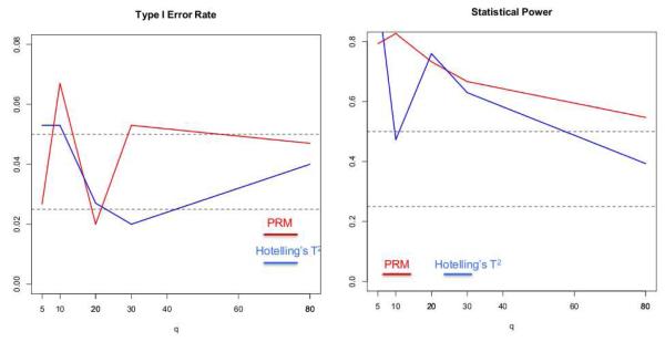
In the first scenario, we set the sample size N to be 150 and the MAF to be 0.5. The q were chosen to be 5, 10, 20, 30, 80 and 100, respectively. The first five individual phenotypes were associated with the SNP, whose coefficients were independently generated from a normal distribution with mean 0.15 and variance 0.05, and the 5th phenotype was also associated with disease status with regression coefficient being 0.5. We applied both the PRM and Hotelling’s T² test to each simulated dataset in order to examine the type I and II error rates under the 5% significance level. Inspecting Figure 1 reveals that the type I errors are well controlled for both methods. Moreover, as q increases, the power in detecting the SNP effect decreases faster for Hotelling’s T² test compared with the PRM.

Fig. 1.

The comparison results of the PRM and Hotelling’s T² test based on N = 150 and MAF=0.5: the type I error (the left panel) and power (the right panel). The upper and middle dashed lines in the left panel correspond to 0.05 and 0.025, respectively; and the upper and middle dashed lines in the right panel represent 0.5 and 0.25, respectively.

3.1.2 Scenario II

In the second scenario, we set q to be 50, 100, 150 and 200, respectively, and the sample size N to be 150, 200, 250 and 300, respectively. We generated the additive SNP effect under 6 different MAFs, which are 0.05, 0.1, 0.2, 0.3, 0.4 and 0.5, respectively. We considered two scenarios of the SNP effect. In the first scenario, only the first individual phenotype is associated with the SNP effect with regression coefficient being 0.5 and the second individual phenotype is associated with the disease status effect with regression coefficient being 0.5. Other individual phenotypes are not associated with any covariate. The second scenario is that the first 10 individual phenotypes are associated with the SNP. We generated the corresponding regression coefficients independently from a normal distribution with mean 0.5 and standard deviation 0.15. Moreover, we set the regression coefficient for the diagnosis status to be 0.5 for the 10th individual phenotype and all other regression coefficients to be zero.

We applied the PRM to the simulated data sets and compared it with two other methods including a component wise method (CWM) and a principal components regression (PCR) using a 5% significance level. The CWM method fits a single linear regression to each individual phenotype with the same set of covariates and uses the false discovery rate (FDR) to test the additive SNP effect. The PCR method extracts the first three principal components of the multivariate phenotype by using the PCA and then fits a multivariate linear model to the extracted principal components with the same set of covariates. The Hotelling’s T² test is not considered here since it is invalid for q > N.

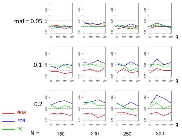
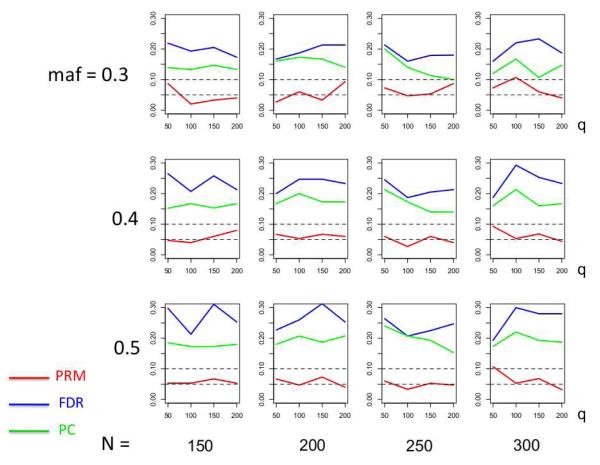
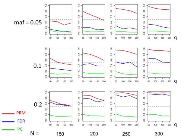
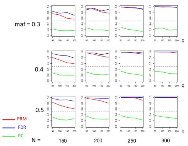
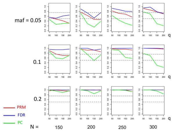
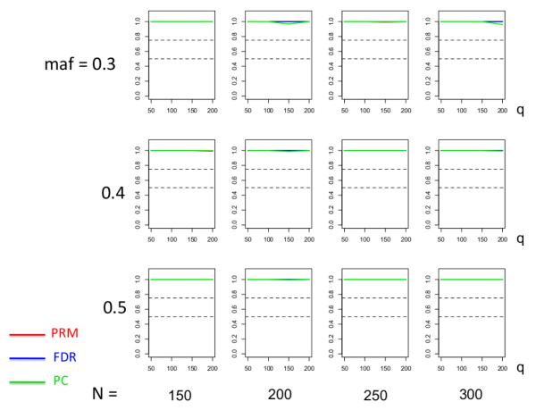
We observe that the type I error rates are well controlled and more stable in the PRM, compared to the CWM and PCR methods (Figures 2 and 3). When the SNP effect is sparse, the powers of the PRM are generally higher than the CWM method, particularly for SNPs with small MAF and it is uniformly better than the PCR method (Figures 4 and 5). As expected, increasing either the sample size N or the MAF enhances the statistical power in detecting the SNP effect, whereas increasing the number of responses q areduces the power in detecting the SNP effect. When more SNPs show impact on the phenotypes, PRM is still comparable to CWM and better then PCR when the MAF is small (Figures 6 and 7). With increasing MAF, all three methods perform equally well.

Fig. 2.

The type I error comparison results of the PRM, CWM, and PCR methods based on different sample sizes (150, 200, 250 and 300) and different minor allele frequencies (0.05, 0.1 and 0.2). The horizontal axis of each plot is the number of phenotypes q and the vertical axis is the type I error rate. The upper and middle dashed lines are 0.1 and 0.05, respectively.

Fig. 3.

The type I error comparison results of the PRM, CWM, and PCR methods based on different sample sizes (150, 200, 250 and 300) and different minor allele frequencies (0.3, 0.4 and 0.5). The horizontal axis of each plot is the number of phenotypes q and the vertical axis is the type I error rate. The upper and middle dashed lines are 0.1 and 0.05, respectively.

Fig. 4.

The power comparison results of the PRM, CWM, and PCR methods for the first scenario of sparse SNP effect based on different sample sizes (150, 200, 250 and 300) and different minor allele frequencies (0.05, 0.1 and 0.2). The horizontal axis of each plot is the number of phenotypes q and the vertical axis is the power. The dashed line represents a power of 50%.

Fig. 5.

The power comparison results of the PRM, CWM, and PCR methods for the first scenario of sparse SNP effect based on different sample sizes (150, 200, 250 and 300) and different minor allele frequencies (0.3, 0.4 and 0.5). The horizontal axis of each plot is the number of phenotypes q and the vertical axis is the power. The dashed line represents a power of 50%.

Fig. 6.

The power comparison results of the PRM, CWM, and PCR methods for multiple SNP effects based on different sample sizes (150, 200, 250 and 300) and different minor allele frequencies (0.05, 0.1 and 0.2). The horizontal axis of each plot is the number of phenotypes q and the vertical axis is the power. The upper and lower dashed lines represent the powers of 75% and 50%, respectively.

Fig. 7.

The power comparison results of the PRM, CWM, and PCR methods for the second scenario of multiple SNP effects based on different sample sizes (150, 200, 250 and 300) and different minor allele frequencies (0.3, 0.4 and 0.5). The horizontal axis of each plot is the number of phenotypes q and the vertical axis is the power. The upper and lower dashed lines represent the powers of 75% and 50%, respectively.

3.2 A neonatal study

The data set is from a neonatal study to assess the impact of common SNPs in putative psychiatric genes on early age brain development. The study recruited 237 pregnant women in their second trimester, who were free from abnormalities on fetal ultrasounds and major medical illness. Each subject had one time visit with a T1-weighted medical resonance image (MRI), demographic and genetic information assessment. The MRI images were collected with a Siemens head-only 3T scanner using a 3D spoiled gradient (FLASH TR/TE/Flip Angle 15/7msec/25) with spatial resolution 1 × 1 × 1 mm³ voxel size. There are 47 regions of interest defined from the T1-weighted images by non-linear warping of a parcellation atlas template [Gilmore et al., 2007, Knickmeyer et al., 2008]. The demographic information includes gender, gestational age at birth in days, age after birth in days and intracranial volume (ICV) of the infants. There are 128 male and 109 female infants with average gestational age 264.0 (SD ±18.91), age after birth in days of 30.2 (SD ±17.80) and ICV 481799.9 (SD ±61528.96). Moreover, 9 genetic variants expressed in SNPs from 6 genes were collected and genotyped by Genome Quebec using Sequenom iPLEX Gold Genotyping Technology.

We applied our PRM method to multivariate phenotype including the volumes of 47 regions of interest (ROIs) with covariates of interest including gender, gestational age, age after birth, ICV and the 9 SNPs with an additive effect. Each hypothesis tests a single SNP effect, while adjusting for other covariates including demographic information and other SNPs. We list the 9 SNPs with their corresponding genes and respective p-values in Table 1.

Table. 1.

Selected SNPs with the corresponding genes and result for testing a single SNP effect while adjusting for demographic information and other SNPs

Gene	Abbreviation	SNP	P-value
Catechol-O-methyltransferase	COMT	rs4680	0.88
Disrupted-in-schizophrenia-1	DISC1	rs821616 rs6675281	0.75 0.016
Neuregulin 1	NRG1	rs35753505 rs6994992	0.0136 0.51
Estrogen Receptor Alpha	ESR1	rs9340799 rs2234693	0.44 0.57
Brain-derived Neurotrophic Factor Glutamate Decarboxylase 1	BDNF GAD1 (GAD67)	rs6265 rs2270335	0.60 0.39

The results show that the SNPs rs6675281 and rs35753505 have a significant impact on early age brain development with p-values of 0.016 and 0.0136, respectively. This agrees with the existing literature. Specifically, DISC1 was known to be associated with mental illness, such as schizoprenia and bipolar disorder, and NRG1 was known to relate to brain tissue volume [Mata et al., 2009].

We also applied the PCR and CWM methods to the same data set with the same set of covariates for comparison. In the PCR application, the first three principal components of the 47 ROIs, which explain 74.4% of the variation, are regressed on the same group of covariates of interest and the same null hypotheses were tested for each SNP by Hotelling’s T² test at the 0.05 significance level. None of the 9 SNPs were found to be significant for brain volume development. The details of the test results are given in the supplementary document. When analyzing the same data set by CWM with multiple comparisons adjusted by FDR, none of the 9 SNPs are detected to be significant for the 47 ROIs at the same testing level.

4 Discussion

We have developed the PRM which provides a more effective analysis for the association delineation between multivariate phenotypes and covariates of interest. The proposed methodology is demonstrated in a study investigating the impact of candidate SNPs on early age brain development. Analysis results obtained from the PRM successfully identified two previously reported SNPs while none of them were detected by either CWM or PCR. This phenomenon is consistent with the results in the simulation studies showing that compared to the two other methods, the PRM tends to have higher power for detecting the association between high dimensional phonetypes and the covariates of interest with better type I error control. Hence we expect that this novel statistical tool will assist scientists in exploring new findings with more effective and reliable statistical results in the high dimensional data settings. Future work includes establishing the asymptotic properties of the PRM under mild conditions, considering ultra-high dimensional phenotypes and genomic data, as well as extending the PRM to longitudinal and familial studies. User-friendly software to implement the PRM will be available to public for non-profit purposes on our group website: http://www.bios.unc.edu/research/bias/software.html.