Complexity-Entropy Causality Plane as a Complexity Measure for Two-Dimensional Patterns

Abstract

Complexity measures are essential to understand complex systems and there are numerous definitions to analyze one-dimensional data. However, extensions of these approaches to two or higher-dimensional data, such as images, are much less common. Here, we reduce this gap by applying the ideas of the permutation entropy combined with a relative entropic index. We build up a numerical procedure that can be easily implemented to evaluate the complexity of two or higher-dimensional patterns. We work out this method in different scenarios where numerical experiments and empirical data were taken into account. Specifically, we have applied the method to fractal landscapes generated numerically where we compare our measures with the Hurst exponent; liquid crystal textures where nematic-isotropic-nematic phase transitions were properly identified; 12 characteristic textures of liquid crystals where the different values show that the method can distinguish different phases; and Ising surfaces where our method identified the critical temperature and also proved to be stable.

Introduction

Investigations related to the so called complex systems are widely spread among different scientific communities, ranging from physics and biology to economy and psychology. A considerable part of these works deals with empirical data aiming to extract patterns, regularities or laws that rule the dynamics of the system. In this direction, the concept of complexity measures often emerges. Complexity measures can compare empirical data such as time series and classify them in somewhere between regular, chaotic or random [1], while other complexity measures can differentiate between degrees of correlations [2]. Examples of these measures include algorithmic complexity [3], entropies [4], relative entropies [5], fractal dimensions [6], and Lyapunov exponents [7]. These seminal works are still motivating new definitions, and today there are numerous definitions of complexity, which have been successful applied to different areas such as medicine [8], [9], ecology [10]–[13], astrophysics [14]–[16], and music [17], [18].

It is surprising that this large number of complexity measures is mainly focused on one-dimensional data, while much less attention has been paid to two and higher-dimensional structures such as images. Naturally, there are few exceptions such as the work of Grassberger [19] and more recent Refs. [20]–[22], though some of the authors of these papers agree that a higher-dimensional approach still represents an open and subtle problem. Furthermore, as it was stated by Bandt and Pompe [23], most of the complexity measures depend on specific algorithms or recipes for processing the data which may also depend on tuning parameters. As a direct consequence, there are huge difficulties for reproducing previous results without the knowledge of details of the methods.

Bandt and Pompe not only raised this problem, but they also proposed an alternative method that tries to overcome the previous problems, introducing what they call permutation entropy – a natural complexity measure for time series. There are many recent applications of this new technique that confirm its usefulness [24]–[31]. In particular, Rosso et al. [1] have successful applied the Bandt and Pompe ideas together with a relative entropic measure [32] to differentiate chaotic time series from stochastic ones. They have constructed a diagram, which was first proposed by López-Ruiz et al. [33], (called as complexity-entropy causality plane) by plotting the relative entropic measure versus the permutation entropy. Intriguingly, chaotic and stochastic series are located in different regions of this representation space.

Here, we show that the complexity-entropy causality plane can be extended for higher-dimensional patterns. We apply this new approach in different scenarios related to two-dimensional structures and the results indicate that the method is very promising for distinguishing between two-dimensional patterns. The following sections are organized as follows. Section II is devoted to review briefly the properties of the permutation information-theory-derived quantifiers and the complexity-entropy causality plane, and also to define an appropriate way to generalize these definitions to higher-dimensional data. In Section III, we work out several applications based on numerical and empirical data. Section IV presents a summary of our results.

Methods

The ingenious idea of Bandt and Pompe [23] was to define a measure that may be easily applied to any type of time series. The method lies on associating symbolic sequences to the segments of the time series based on the existence of local order, and next, by using probability distribution associated to these symbols, to estimate the complexity quantifier. For purpose of definition, let us consider a time series composed by elements and also -dimensional vectors () defined by

where . Next, for all the vectors, we evaluate the permutations of defined by . The possible permutations of will be the accessible states of the system, and for each state we estimate the ordinal pattern probability given by

where the symbol # stands for the number of occurrences of the permutation . Now, we can apply the ordinal patterns probability distribution, , to estimate a complexity measure based on some entropic formulation.

Before advancing, we note that the previous method may be extended to higher-dimensional data structures such as images. In order to do this, we consider that the system is now represented by a two-dimensional array of size . In analogy to the vector , we define matrices () given by

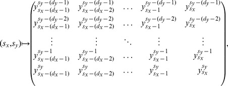where and . Next, for all these matrices, we evaluate the permutations of defined by . The system can now access states for which we calculate the probability distribution through the relative frequencies given by

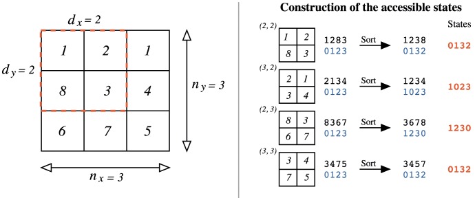
For easier understanding, we illustrate this procedure for a small array in Fig. 1.

Figure 1. Schematic representation of the construction of the accessible states.

In this example we have a array (left panel) and we choose the embedding dimensions and . In the right panel we illustrate the construction of the states. We first obtain the sub-matrix corresponding to and that have as elements and, after sorting, this sub-matrix leads to the state “0132”. We thus move to next sub-matrix and which have the elements and that, after sorting, leads to the state “1023”. The last two remaining matrices lead to the states “1230” and “0132”. Finally, we estimate the probabilities , that are, , and which are then used in the equations (1) and (2), leading to and .

Naturally, the order procedure that defines the permutation is no longer unique as in the one-dimensional case. For instance, instead of ordering the elements of row-by-row, we could also order column-by-column. However, these other definitions will only change the “name” of the states in such a way that the set will remain unchanged. Thus, there is no lost of generalization in assuming a given order recipe for defining .

We note that this procedure is straightforward generalized to accomplish higher-dimensional structures (e.g., the volumetric brain images obtained via functional magnetic resonance imaging), and that it recovers the one-dimensional case by setting and . Here, for simplicity, we focus our analysis on two-dimensional structures.

The parameters and (known as embedding dimensions) play an important role in the estimation of the permutation probability distribution , since they determine the number of accessible states. In the one-dimensional case, it is usual to choose in order to obtain reliable statistics in the one-dimensional case (for practical purposes, Bandt and Pompe recommend [23]). For the two-dimensional case a similar relationship must hold, i.e., . To go further, we need to rewrite the entropic measures used in Refs. [1], [23]. The first one is called normalized permutation entropy [23] and it is obtained by applying the Shannon’s entropy to the probabilities , i.e.,

(1)

where and . The value of is obtained by considering all the accessible states to be equiprobable, i.e., . By definition, , where the upper bound occurs for a completely random array. We expect for arrays that exhibit some kind of correlated dynamics.

The other measure [1] is defined by.

(2)

where is a relative entropic metric between the empirical ordinal probability and the equiprobable state . The quantity is known as disequilibrium and it is defined in terms of the Jensen-Shannon divergence [34] (or also in terms of a symmetrized Kullback-Leibler divergence [35]) and can be written as

(3)

where

is the maximum possible value of , obtained when one of the components of is equal to one and all the other vanish.

The disequilibrium quantifies the degree of correlational structures providing important additional information that may not be carried only by the permutation entropy. In addition, for a given value there exists a range of possible values for [36]. This is the main reason why Rosso et al. [1] proposed to employ a diagram of versus as a diagnostic tool, building up the complexity-entropy causality plane.

Results and Discussion

In the following, we will calculate the diagram of versus to measure the complexity and to distinguish among different two-dimensional patterns.

Fractal Surfaces

We generate fractal surfaces through the random midpoint displacement algorithm [37]. This algorithm starts with a square. For each vertex, we assign a random value representing the surface height. Next, we add a new point located at the center of the initial square. We set the height of this point equal to the average height of the previous four vertex plus a Gaussian random number with zero mean and standard-deviation . We also add four points located at the middle segments which connects each initial vertex. For these four points, the heights are equal to the average value between the two closest vertex and the middle point plus a Gaussian random number with zero mean and standard-deviation . Now, we imagine that these 9 points represent four new squares and, for each one, we apply the previous procedure using . By repeating this process times and using , we should obtain a square surface of side with fractal properties. 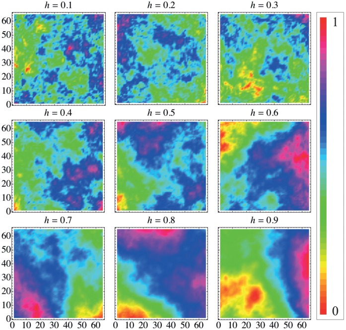Here, is the Hurst exponent and is the surface fractal dimension. Figure 2 shows several surfaces generated through this procedure for different values of .

Figure 2. Examples of fractal surfaces obtained through the random midpoint displacement method.

These are surfaces () for different values of the Hurst exponent . For easier visualization, we have scaled the height of the surfaces in order to stay between and . We note that for small values of the surfaces display an alternation of peaks and valleys (anti-persistent behavior) much more frequent than those one obtained for larger values of . For larger values of , the surfaces are smoother reflecting the persistent behavior induced by the value of .

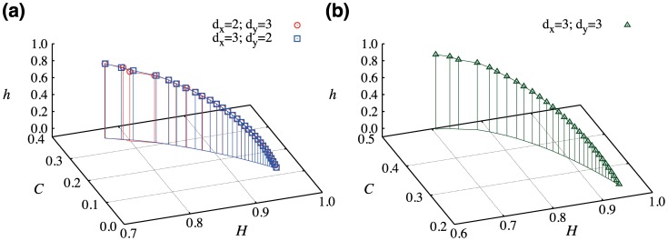
We apply our method for these surfaces aiming to verify how the permutation quantifiers and change with the Hurst exponent , as it is shown in Fig. 3. In these 3d plots, we show the localization in the causality plane obtained for different values of evaluated from surfaces (). In Fig. 3a, we use and (circles), and and (squares) as embedding dimensions. Note that the values of and are practically invariant under the rotation and . This invariance is related to the fact that in these fractal surfaces there is not preferential direction. In Fig. 3b, we employ and . We note basically the same dependence but a different range for and , since this change increases the number of accessible states. These results show that our method properly differentiates fractal surfaces concerning the Hurst exponent. Moreover, we investigate the robustness of the permutation quantifiers under several realizations of the random midpoint displacement algorithm and the results show that both indexes are very stable. For example, the standard-deviation in the values of and are usually smaller than when considering .

Figure 3. Dependence of the complexity-entropy causality plane on Hurst exponent h .

We have employed fractal surfaces of size (). In (a) we plot and versus for the embedding dimensions and (circles) and also for and (squares). We note the invariance of the index against the rotation and . In (b) we plot the diagram for . We observe changes in the scale of and caused by the increasing number of states. In both cases, as increases the complexity also increases while the permutation entropy decreases. This behavior reflects the differences in the roughness shown in Fig. 2. For values of the surface is anti-persistent which generates a flatter distribution for the values of leading to values of and closer to the aleatory limit ( and ). For values of there is a persistent behavior in the surfaces heights which generates a more intricate distribution of and, consequently, values of and that are closer to the middle of the causality plane (region of higher complexity).

Liquid Crystal Textures

Another interesting application is related to different patterns that a thin film of a liquid crystal exhibits. These textures are obtained by observing a thin sample of liquid crystal placed between two crossed polarizers in a microscope. The textures give useful information about the macroscopic structure of the liquid crystal. For instance, different phases have different typical textures, and by tracking their evolution one can properly identify the phase transition.

We first study a lyotropic liquid crystal under isotropic-nematic-isotropic phase transition. Figure 4 shows three snapshots of the texture at different temperatures. In this case, we clearly note the differences in the textures. The leftmost and rightmost textures are at the isotropic phase while the middle one is at the nematic phase. We observe that the pattern is very complex for the nematic phase, while for the isotropic one it is basically random.

Figure 4. Characteristic textures of a lyotropic liquid crystal at different temperatures and phases.

The lyotropic system used here is a mixture of potassium laurate , decanol and deuterium oxide – suitable concentrations in order to get a isotropic nematic isotropic phase sequence [38]. These images were constructed by observing the optical microscopy of a flat capillary which contains the mixture at different temperatures. Here, we have used the average value of the pixels of the three layers (RGB) of the original image and a rescaled temperature.

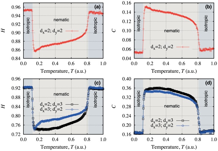
We calculate and as a function of the temperature for different values of the embedding dimensions, as it is shown in Fig. 5. In these plots, the different shaded regions represent the different liquid crystal phases. We note that the phase transitions are successful identified independently of and . However, Fig. 5c and 5d show a slight different dependence of and versus the temperature when considering and or and . Because the liquid crystal sample is placed in elongated capillary tube, there is a surface effect that act on the liquid crystal molecules. This effect is usually amplified at the phase transition and it is also the reason for differences between the embedding dimensions.

Figure 5. Dependence of the entropic indexes on the temperature of a lyotropic liquid crystal.

We plot versus the temperature in (a) and versus the temperature in (b), where we employ . Figures (c) and (d) present the results for and , and also for and . The different shaded areas represent the different liquid crystal phases. Note that the phase transitions are properly identified in all cases. Due to the asymmetry of the elongated capillary tube where the liquid crystal sample is placed, and present slight differences under the rotation and .

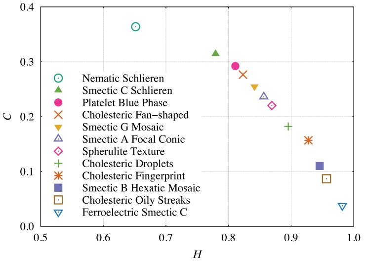
In this particular phase transition, the difference between the textures are large enough that it can be identified just by visual inspection. However, this is not the usual case and many phase transitions are very difficult to identify. In this context, an interesting question is whether our method can help to distinguish different phases. To address this question, we evaluate and for twelve characteristic textures of different liquid crystals. We download these textures from the webpage of the Liquid Crystal Institute at Kent State University [39] and Fig. 6 shows the value of and for each texture in the causality plane. The results allow to conclude that the method ranks the textures in a kind of complexity order where each characteristic texture occupies a different place in this representation space. Moreover, the different values of and indicate that the permutation quantifiers can also identify smooth phase transitions.

Figure 6. Complexity-entropy causality plane evaluated for several liquid crystal textures [[39]].

Here, we have used the averaged pixel values of the three layers (RGB) of the original image and and . The image sizes are about pixels. We note that each texture has a unique position in the causality plane which indicates that the permutation quantifiers are capable of differentiate not only transitions involving the isotropic phase, but also smoother phase transitions. We further observe that some high ordered phase such as the blue phase are located at the central part of the causality plane (region of higher complexity), while other phases which present a large number of defects such as the Smectic B and C are closer to the aleatory limit ( and ).

Naturally, the location of each texture in the causality plane should be related to physical properties of the liquid crystals. A better understanding of the relation between the permutation quantifiers and these physical attributes may deserves a more careful investigation since some properties of liquid crystals such as the order parameter can be quite hard to empirically measure. In this context, the existence of a clear relation between, for example, the order parameter and or will be experimentally handy. Here, we just have the pictures of the textures in such a way that is very hard to point out these relationships. However, a visual inspection of Fig. 6 suggests that some of the more ordered phases, such as the blue phase (this phase display a cubic structure of defects), are located in the central part of the causality plane (region of higher complexity), while other textures which present a large number of non-ordered defects, such as the Smectic B and C, are positioned closer to the aleatory limit ( and ). Thus, it seems that the permutation quantifiers are capturing in somehow the competition between the orientational order of the phase and, also, the number of defects present in the textures.

Ising Surfaces

As a last application, we study the permutation measures and applied to Ising surfaces [40], [41]. These surfaces are obtained by accumulating the lattice spin values of the Ising model defined by the Hamiltonian.

(4)

where the sum is over all the pairs of first neighbor sites in the lattice. We numerically solve this spin- Ising model on a lattice using the Monte Carlo method with periodic boundary conditions. By using the spin values, we define the surface height for each lattice site as

(5)

where represents the number of Monte Carlo steps. In Fig. 7, we show three surfaces obtained though this procedure for different values of the reduced temperature , where is the critical temperature of the model. We note the complex pattern exhibited by the surface for , and the almost random patterns for and .

Figure 7. Examples of Ising surfaces for three different temperatures.

These surfaces were obtained after Monte Carlo steps for three different temperatures: below , at and above . In these plots, the height values were scaled to stay between and . We note that for temperatures higher or lower than , the surfaces exhibit an almost random pattern. For values of the temperature closer to the surfaces exhibit a more complex pattern, reflecting the long-range correlations that appear among the spin sites during the phase transition.

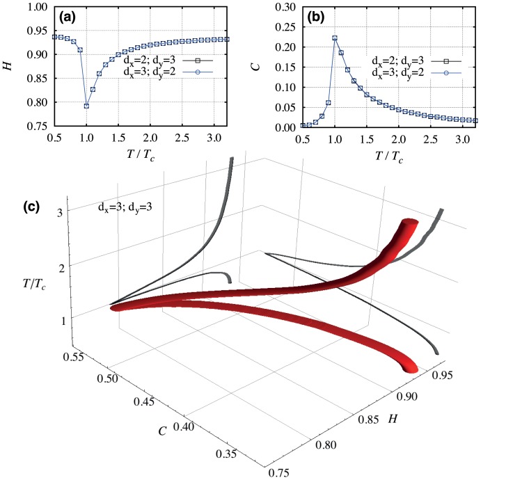
We first investigate the dependence of and on the reduced temperature after a large number of Monte Carlo steps () and for . Figures 8a and 8b show and for and , and for the rotation and . We note that, at the critical temperature, both indexes display a sharp peak and that they are invariant under the rotation. Moreover, Fig. 8c presents a 3d visualization of the phase transition for . This higher-dimensional representation can be useful when investigating more complex phase transitions, since a greater number of degrees of freedom allows the critical point to be more visible.

Figure 8. Dependence of the entropic indexes on the reduced temperature for Ising surfaces.

(a) The permutation entropy and (b) the complexity measure versus the reduced temperature for and , and also for and . We note invariance of indexes under the rotation and . (c) A 3d visualization of the Ising model phase transition when considering . The gray shadows represent the dependences of on and of on .

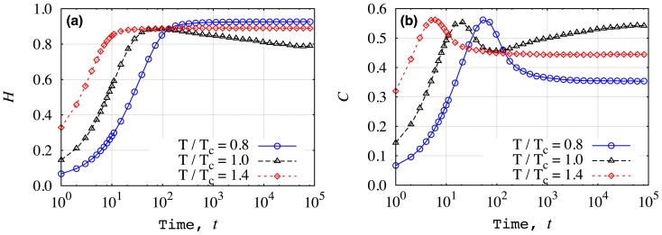
We further study the temporal evolution of and for different reduced temperatures, as it is shown in Fig. 9. The initial values of the spins were chosen equal to and, as we can see, the values for and are different just after one Monte Carlo step. For , the value of increases over time and around it reaches a plateau. For , the value of increases up to a maximum value around and then starts to approach a lower plateau value. A striking behavior is observed for , where for all temperatures the complexity displays a maximum value before it begins to approach a plateau value. It is worth noting that both quantifiers are very stable after Monte Carlo steps.

Figure 9. Dependence of the entropic indexes on the number of Monte Carlo steps.

Here, denotes the number of Monte Carlo steps and the reduced temperatures are indicated in the plots. In (a) we show versus and in (b) versus for . We note the stability of both indexes after Monte Carlo steps.

Conclusions

We have proposed a generalization of the complexity-entropy causality plane to higher-dimensional patterns. We applied this approach to fractal surfaces, liquid crystal textures and Ising surfaces. It was shown that the indexes and performed very well for distinguishing between the different roughness of the fractal surfaces. The indexes properly identified the phase transitions of a lyotropic liquid crystal and sorted different characteristic textures in a kind of complexity order. Finally, concerning the Ising surfaces, the indexes not only had identified the critical temperature, but also proved to be stable after Monte Carlo steps. The method also has a very fast and simple numerical evaluation. Taking into account all these findings, we are very optimist that our method can reduce the gap between one-dimensional complexity measures and the higher-dimensional ones.

Funding Statement

This work has been supported by the agencies Conselho Nacional de Desenvolvimento Científico e Tecnológico, Coordenação de Aperfeiçoamento de Pessoal de Nível Superior (CAPES), and Consejo Nacional de Investigaciones Científicas y Técnicas. HVR also thank the financial support of CAPES (Grant 5678-11-0). The funders had no role in study design, data collection and analysis, decision to publish, or preparation of the manuscript.

References

- 1. Rosso OA, Larrondo HA, Martin MT, Plastino A, Fuentes MA (2007) Distinguishing Noise from Chaos. Phys. Rev. Lett. 99: 154102. [DOI] [PubMed] [Google Scholar]
- 2. Rosso OA, Zunino L, Pérez DG, Figliola A, Larrondo HA, et al. (2007) Extracting features of Gaussian self-similar stochastic processes via the Bandt-Pompe approach. Phys. Rev. E 76: 061114. [DOI] [PubMed] [Google Scholar]
- 3. Kolmogorov AN (1965) Three Approaches to the Quantitative Definition of Information. Probl. Inf. Transm. 1: 3–11. [Google Scholar]
- 4. Shannon CE (1948) A Mathematical Theory of Communication. Bell Syst. Tech. J. 27: 379–423. [Google Scholar]
- 5. Kullback S, Leibler RA (1951) On Information and Sufficiency. Ann. Math. Statist. 22: 79–86. [Google Scholar]
- 6.Mandelbrot BB (1982) The Fractal Geometry of Nature. San Francisco: Freeman.
- 7.Lyapunov AM (1992) The General Problem of the Stability of Motion. London: Translated by A. T. Fuller, Taylor-Francis.
- 8. Maes F, Collignon A, Vandermeulen A, Marchal G, Suetens P (1997) Multimodality Image Registration by Maximization of Mutual Information. IEEE Trans. Med. Imag. 16: 187–198. [DOI] [PubMed] [Google Scholar]
- 9. Khader M, Hamza AB (2011) Nonrigid Image Registration Using an Entropic Similarity. IEEE Trans. Inf. Technol. Biomed. 15: 681–690. [DOI] [PubMed] [Google Scholar]
- 10. Parrott L (2005) Quantifying the Complexity of Simulated Spatiotemporal Population Dynamics. Ecological Complexity 2: 175–184. [Google Scholar]
- 11. Jost L (2006) Entropy and diversity. Oikos 113: 363–375. [Google Scholar]
- 12. Mendes RS, Evangelista LR, Thomaz SM, Agostinho AA, Gomes LC (2008) A Unified Index to Measure Ecological Diversity and Species Rarity. Ecography 31: 450–456. [Google Scholar]
- 13. Parrott L (2010) Measuring Ecological Complexity. Ecological Indicators 10: 1069–1076. [Google Scholar]
- 14. Schwarz U, Benz AO, Kurths J, Witt A (1993) Analysis of Solar Spike Events by Means of Symbolic Dynamics Methods. Astron. Astrophys. 277: 215–224. [Google Scholar]
- 15. Consolini G, Tozzi R, De Michelis P (2009) Complexity in the Sunspot Cycle. Astron. Astrophys. 506: 1381–1391. [Google Scholar]
- 16. Lovallo M, Telesca L (2011) Complexity Measures and Information Planes of X-ray Astrophysical Sources. J. Stat. Mech. P03029. [Google Scholar]
- 17. Boon JP, Decroly O (1995) Dynamical Systems Theory for Music Dynamics. Chaos 5: 501. [DOI] [PubMed] [Google Scholar]
- 18. Su ZY, Wu T (2006) Multifractal Analyses of Music Sequences. Physica D 221: 188–194. [Google Scholar]
- 19. Grassberger P (1986) Toward a Quantitative Theory of Self-generated Complexity. Int. J. Theor. Phys. 25: 907. [Google Scholar]
- 20. Andrienko YA, Brilliantov NV, Kurths J (2000) Complexity of Two-dimensional Patterns. Eur. Phys. J. B 15: 539–546. [Google Scholar]
- 21. Feldman DP, Crutchfield JP (2003) Structural Information in Two-dimensional Patterns: Entropy Convergence and Excess Entropy. Phys. Rev. E 67: 051104. [DOI] [PubMed] [Google Scholar]
- 22. Cai Z, Shen E, GU F, Xu Z, Ruan J, et al. (2006) A New Two-Dimensional Complexity Measure. Int. J. Bifurcation Chaos 16: 3235. [Google Scholar]
- 23. Bandt C, Pompe B (2002) Permutation Entropy: A Natural Complexity Measure for Time Series. Phys. Rev. Lett. 88: 174102. [DOI] [PubMed] [Google Scholar]
- 24. Ouyang G, Dang C, Richards DA, Li X (2010) Ordinal Pattern Based Similarity Analysis for EEG Recordings. Clin. Neurophysiol. 121: 694–703. [DOI] [PubMed] [Google Scholar]
- 25. Li X, Ouyang G (2010) Estimating Coupling Direction Between Neuronal Populations with Permutation Conditional Mutual Information. NeuroImage 52: 497–507. [DOI] [PubMed] [Google Scholar]
- 26. Nicolaou N, Georgiou J (2011) The Use of Permutation Entropy to Characterize Sleep Electroencephalograms. Clin. EEG Neurosci. 42: 24–28. [DOI] [PubMed] [Google Scholar]
- 27. Masoller C, Rosso OA (2011) Quantifying the Complexity of the Delayed Logistic Map. Phil. Trans. R. Soc. A 369, 425–438. [DOI] [PubMed] [Google Scholar]
- 28. Barreiro M, Marti AC, Masoller C (2011) Inferring Long Memory Processes in the Climate Network via Ordinal Pattern Analysis. Chaos 21: 013101. [DOI] [PubMed] [Google Scholar]
- 29. Cánovas JS, Guillamón A, del Carmen-Ruíz M (2011) Using Permutations to Detect Dependence Between Time Series. Physica D 240: 1199–1204. [Google Scholar]
- 30. Nicolaou N, Georgiou J (2012) Detection of Epileptic Electroencephalogram Based on Permutation Entropy and Support Vector Machines. Expert Syst. Appl. 39: 202–209. [Google Scholar]
- 31. Ribeiro HV, Zunino L, Mendes RS, Lenzi EK (2012) Complexity-entropy Causality Plane: A useful Approach for Distinguishing Songs. Physica A 391: 2421–2428. [Google Scholar]
- 32. Lamberti PW, Martin MT, Plastino A, Rosso OA (2004) Intensive Entropic Non-Triviality Measure. Physica A 334: 119–131. [Google Scholar]
- 33. López-Ruiz R, Mancini HL, Calbet X (1995) A Statistical Measure of Complexity. Phys. Lett. A 209: 321–326. [Google Scholar]
- 34. Grosse I, Bernaola-Galván P, Carpena P, Román-Roldán R, et al. (2002) Analysis of Symbolic Sequences Using the Jensen-Shannon Divergence. Phys. Rev. E 65: 041905. [DOI] [PubMed] [Google Scholar]
- 35. Lin J (1991) Divergence Measures Based on the Shannon Entropy. IEEE Trans. Inf. Theory 37: 145–151. [Google Scholar]
- 36. Martin MT, Plastino A, Rosso OA (2006) Generalized Statistical Complexity Measures: Geometrical and Analytical Properties. Physica A 369: 439–462. [Google Scholar]
- 37. Fournier A, Fussel D, Carpenter L (1982) Computer Rendering of Stochastic Models. Commun. ACM 25: 371–384. [Google Scholar]
- 38. Yu LJ, Saupe A (1980) Observation of a Biaxial Nematic Phase in Potassium Laurate-1-Decanol-Water Mixtures. Phys. Rev. Lett. 45: 1000–1003. [Google Scholar]
- 39.Kent State University, Available: http://dept.kent.edu/spie/liquidcrystals/accessed on 2012 January 10.
- 40. Brito AF, Redinz JA, Plascak JA (2007) Dynamics of Rough Surfaces Generated by Two-dimensional Lattice Spin Models. Phys. Rev. E 75: 046106. [DOI] [PubMed] [Google Scholar]
- 41. Brito AF, Redinz JA, Plascak JA (2010) Two-dimensional XY and Clock Models Studied via the Dynamics Generated by Rough Surfaces. Phys. Rev. E 81: 031130. [DOI] [PubMed] [Google Scholar]