Regularized Optimization (RO) Reconstruction for Oximetric EPR Imaging

Abstract

A new algorithm for EPR imaging oximetry is described and tested with experimental data for the case of one spatial and one spectral dimension. A single species with variable linewidth is assumed. Instead of creating a 2D image, two one-dimensional profiles are reconstructed: the concentration of the radical and the corresponding oxygen concentration, which reduces the dimensionality of the problem. The algorithm (i) seeks to minimize the discrepancy between experimental data and projections calculated from the profiles and (ii) uses Tikhonov regularization to constrain the smoothness of the results. This approach controllably smoothes profiles rather than the data, while preserving sharp features.

1. Introduction

Electron paramagnetic resonance imaging (EPRI) is under development for diverse biomedical applications including cardiology [1], liposomal drug delivery [2], oxidative stress and reperfusion injury [3], and cancer [4, 5]. Many applications of EPR imaging involve oximetry [6], in which local oxygen concentration is detected via the broadening of a narrow paramagnetic probe signal by collisions with paramagnetic oxygen. Imaging information is encoded by recording spectra (projections) in the presence of magnetic field gradients. Spectral-spatial or spectroscopic images are reconstructed in which the spectrum is determined at each position in the sample. Since the concentrations of probes are low, and there are time constraints on data acquisition for real-world applications, images must be reconstructed from limited numbers of noisy projections. Image reconstruction in this situation is known to be an ill-posed problem [7]. This means that from an infinitely large number of solutions that match almost equally well with the experimental data, the one that probably is the best must be selected.

Many reconstruction algorithms have been developed for various imaging modalities. Filtered backprojection method (FBP), which was developed for X-ray tomography [8], is the most commonly used method for EPR imaging. The advantages of FBP are: modest computation time, simplicity in implementation, and robustness. Its well-known disadvantages include characteristic distortions (“star effect”) that occur when there are too few projections and the need for equally-spaced projections [9]. If there are no sharp features in the experimental projections, images reconstructed by FBP can be improved by smoothing the data before the algorithm is applied. However for images of unknown objects it is difficult to define the filtering parameters that can be used without distorting features in noisy spectra. Iterative methods, such as maximum entropy, may give more accurate results but are more computationally intensive [10, 11].

An alternate approach to finding solutions of ill-posed problems is Tikhonov regularization [7, 12, 13], which when applied to image reconstruction seeks to minimize the function

$${\Vert \widehat{\mathrm{R}}\mathrm{I}(\overrightarrow{\mathrm{\rho }})-\overrightarrow{\mathrm{D}}\Vert }^2+\mathrm{\lambda }{\Vert \widehat{\mathrm{L}}(\overrightarrow{\mathrm{\rho }})\Vert }^2$$ (1)

where R̂ is the discrete Radon transform operator for projections at angles Θ⃗, I(ρ⃗) is the image, D⃗ is the experimental projection data, λ is the regularization parameter, L̂ is the regularization operator, ρ⃗ is a vector of parameters to be regularized, and the notation ‖ ‖ indicates the Euclidean norm.

The term ‖L̂(ρ⃗)‖² is the regularization term. The term ‖R̂I(ρ⃗)−D⃗‖ is the error or penalty term (Σ) and reflects the discrepancy between projections from the reconstructed image and the experimental data. The selection of the regularization operator can be used to impose constraints, based on knowledge of the system. For example, L̂ = L₀ (the identity matrix) forces values of ρ⃗ toward zero, L̂ = L₁ (the first derivative matrix) forces values toward a constant, and L̂ = L₂ (the second derivative matrix) forces the slope toward a constant. Thus the selection of L̂ provides a way to smooth the image, instead of smoothing the experimental projections as is used in filtered backprojection, while also keeping track of the impact of the smoothing on the error function. The larger the regularization parameter λ, the smoother the image. Especially when data are noisy, the value of λ must be large enough to filter out noise, but small enough that it does not suppress significant features. Thus, wise choice of regularization parameter is important to keep the proper balance between minimizing the error term and smoothing the image. The quality of the outcome depends upon the selection of λ. In the literature various ways have been used to select the regularization parameter, including the discrepancy principle method [12–14], which takes noise statistic into account, the L-curve method [15–19], and the generalized cross-validation method [20, 21]. A recent review concludes that λ is usually selected empirically [22].

Another disadvantage of FBP is that it is difficult to incorporate a priori information about the object that is imaged. For EPRI oximetry the lineshape of the spin probe in the absence of oxygen, including unresolved or resolved nuclear hyperfine structure, is known. Collisions with oxygen decrease the T₂ for the probe and cause broadening of the line. The oxygen concentration is calculated from the broadening. The unknown parameters for each position in the object are line width (or line broadening), and the integrated intensity of the line, which is proportional to radical concentration at that point. One currently-used approach is to fit each spectral profile in the spectral-spatial image to a spin probe lineshape [23] and thereby find the oxygen and radical concentration in each voxel [24], which requires two steps: reconstruction and fitting.

A new approach to spectral-spatial imaging has been suggested recently that reconstructs profiles directly and does not require reconstruction of an intermediate image [25]. The goal is to find a “lineshape constrained” image for which calculated projections match the experimental projections as well as possible. The name “lineshape constrained” means that the lineshape for each spectral slice of the image is broadened by a variable amount relative to the lineshape for the probe in the absence of oxygen. In addition to probe lineshape, other constraints can be applied. It has been demonstrated that, compared with standard FBP reconstruction, this method permits significant reduction of data acquisition time by measurement of fewer projections with smaller sweep widths without loss of quality in the final results. In this Bayesian approach the goal is the image with maximum a posteriori probability, taking into account a priori information. It is assumed that experimental projections are contaminated with random Gaussian noise and that spatial profiles of radical concentration ρ⃗_R and linewidth ρ⃗_τ need to be smoothed. The vectors ρ⃗_R and ρ⃗_τ are found by minimizing function (2) using non-linear optimization [25].

$${\Vert \widehat{\mathrm{R}}\mathrm{I}(\overrightarrow{\mathrm{\rho }})-\overrightarrow{\mathrm{D}}\Vert }^2+\mathrm{\lambda }\left({\Vert {\widehat{\mathrm{L}}}_1({\overrightarrow{\mathrm{\rho }}}_{\mathrm{R}})\Vert }^2+{\Vert {\widehat{\mathrm{L}}}_1({\overrightarrow{\mathrm{\rho }}}_{\mathrm{\tau }})\Vert }^2\right)$$ (2)

Eq. (2) is very similar to Tikhonov regularization (Eq. (1)). However, in Eq. (2) two regularization terms are multiplied by a single regularization parameter, which implies that the spatial variation in distributions of oxygen and radicals have similar smoothness. In real systems the spatial variation may be quite different.

A new approach to finding a "lineshape constrained" image is suggested. It is based on minimizing a function similar to (2), but with two regularization parameters. Instead of nonlinear optimization, the Tikhonov regularization method is used. This approach allows more flexibility in incorporating a priori information such as characteristics of oxygen and radical distributions and excluding regions that are inaccessible to radical.

To test the utility of this approach, it is applied to oximetric imaging with one spatial dimension and one spectral dimension. This information can be presented as a 2D spectral-spatial image that displays the EPR spectrum as a function of position along an axis through the sample. For the lineshape constrained case, the same information can be presented more compactly in two 1-D arrays that summarize the information from spectral slices through the spectral-spatial image. Each element in the spatial profile of the radical, ρ⃗_R, is the integrated intensity. Each element in the spatial profile of oxygen, ρ⃗_O, is the full width at half height of the absorption signal, which is proportional to oxygen concentration.

2. Regularized Optimization (RO) Algorithm

To account for differences in the spatial variation of radical and oxygen concentrations, functions (1) and (2) were modified to have separate regularization parameters, λ_R and λ_O, and regularization operators, L̂_R and L̂_O, for the two profiles.

$${\Vert \widehat{\mathrm{R}}\mathrm{I}({\overrightarrow{\mathrm{\rho }}}_{\mathrm{R}},{\overrightarrow{\mathrm{\rho }}}_{\mathrm{O}})-\overrightarrow{\mathrm{D}}\Vert }^2+{\mathrm{\lambda }}_{\mathrm{R}}{\Vert {\widehat{\mathrm{L}}}_{\mathrm{R}}({\overrightarrow{\mathrm{\rho }}}_{\mathrm{R}})\Vert }^2+{\mathrm{\lambda }}_{\mathrm{O}}{\Vert {\widehat{\mathrm{L}}}_{\mathrm{O}}({\overrightarrow{\mathrm{\rho }}}_{\mathrm{O}})\Vert }^2$$ (3)

where I is the image matrix with dimension N × N, ρ⃗_i is a vector of length N, and D⃗ is a vector containing the experimental projections sequentially. It is proposed that the two profiles can be calculated iteratively holding one constant, while optimizing the other. For a lineshape constrained image, the error term in function (3) can be rearranged for two cases: constant ρ⃗_O or constant ρ⃗_R and expressed in terms of matrices and vectors that are suitable for the Tikhonov method.

For constant ρ⃗_O

$${\Vert \widehat{\mathrm{R}}\mathrm{I}({\overrightarrow{\mathrm{\rho }}}_{\mathrm{R}},{\overrightarrow{\mathrm{\rho }}}_{\mathrm{O}})-\overrightarrow{\mathrm{D}}\Vert }^2={\Vert {\displaystyle \sum _{\mathrm{k}=1}^{\mathrm{N}}}{\mathrm{\rho }}_{\mathrm{R}}^{\mathrm{k}}\widehat{\mathrm{R}}{\mathrm{S}}_{\mathrm{k}}({\mathrm{\rho }}_{\mathrm{O}}^{\mathrm{k}})-\overrightarrow{\mathrm{D}}\Vert }^2$$ (4)

where S_k is a matrix with the k^th row equal to the intensity-normalized spectrum at point k along the spectral axis, with $\text{linewidth}={\mathrm{\rho }}_{\mathrm{O}}^{\mathrm{k}}$ and other rows = 0. Radon transformation of matrix S_k produces projections that can be combined into a matrix that is denoted as P as in Eq. (5).

$${\Vert \widehat{\mathrm{R}}\mathrm{I}({\overrightarrow{\mathrm{\rho }}}_{\mathrm{R}},{\overrightarrow{\mathrm{\rho }}}_{\mathrm{O}})-\overrightarrow{\mathrm{D}}\Vert }^2={\Vert \mathrm{P}{\overrightarrow{\mathrm{\rho }}}_{\mathrm{R}}-\overrightarrow{\mathrm{D}}\Vert }^2$$ (5)

P can be calculated directly as the Radon transforms of spectral slices arranged as columns in a matrix. Substitution of Eq. (5) into Eq. (3) with the constraint that ρ⃗_O = constant, taking the derivative with respect to ρ⃗_R, and setting it equal to zero, gives Eq. (6) that can be used to calculate ρ⃗_R.

$${\overrightarrow{\mathrm{\rho }}}_{\mathrm{R}}={({\mathrm{P}}^{\mathrm{T}}\mathrm{P}+{\mathrm{\lambda }}_{\mathrm{R}}{\mathrm{L}}_{\mathrm{R}}^{\mathrm{T}}{\mathrm{L}}_{\mathrm{R}})}^{-1}{\mathrm{P}}^{\mathrm{T}}\overrightarrow{\mathrm{D}}$$ (6)

where P^T and L^T are the transpose of the corresponding matrices. The values of P and P^T depend on the current estimate of ρ⃗_O.

A different approach is required to find ρ⃗_O at constant ρ⃗_R, because although the lineshape depends linearly on radical concentration, it does not depend linearly on the linewidth values in ρ⃗_O. However, the error function in Eq. (3) can be re-written using an approximate expression for the dependence of lineshape on linewidth in the range where changes are small enough to be approximated by the linear term of a Taylor expansion.

For constant ρ⃗_R

$${\Vert \widehat{\mathrm{R}}\mathrm{I}({\overrightarrow{\mathrm{\rho }}}_{\mathrm{R}},{\overrightarrow{\mathrm{\rho }}}_{\mathrm{O}})-\overrightarrow{\mathrm{D}}\Vert }^2~{\Vert {\displaystyle \sum _{\mathrm{k}=1}^{\mathrm{N}}}{\mathrm{\rho }}_{\mathrm{R}}^{\mathrm{k}}\widehat{\mathrm{R}}{\mathrm{S}}_{\mathrm{k}}({\mathrm{\rho }}_{\mathrm{O}}^{\mathrm{k}})+{\displaystyle \sum _{\mathrm{k}=1}^{\mathrm{N}}}{\mathrm{\rho }}_{\mathrm{R}}^{\mathrm{k}}\widehat{\mathrm{R}}\frac{{\text{dS}}_{\mathrm{k}}({\mathrm{\rho }}_{\mathrm{O}}^{\mathrm{k}})}{\mathrm{d}{\mathrm{\rho }}_{\mathrm{O}}^{\mathrm{k}}}\mathrm{\delta }{\mathrm{\rho }}_{\mathrm{O}}^{\mathrm{k}}-\overrightarrow{\mathrm{D}}\Vert }^2$$ (7)

where $\mathrm{\delta }{\mathrm{\rho }}_{\mathrm{O}}^{\mathrm{k}}$ is an element of the vector of increments to the oxygen profile that needs to be determined. Eq. (7) can be rewritten as

$${\Vert \widehat{\mathrm{R}}\mathrm{I}({\overrightarrow{\mathrm{\rho }}}_{\mathrm{R}},{\overrightarrow{\mathrm{\rho }}}_{\mathrm{O}})-\overrightarrow{\mathrm{D}}\Vert }^2~{\Vert \mathrm{P}{\overrightarrow{\mathrm{\rho }}}_{\mathrm{R}}-\overrightarrow{\mathrm{D}}+\mathrm{Q}\mathrm{\delta }{\overrightarrow{\mathrm{\rho }}}_{\mathrm{O}}\Vert }^2=\Vert \mathrm{Q}\mathrm{\delta }{\overrightarrow{\mathrm{\rho }}}_{\mathrm{O}}-\overrightarrow{\mathrm{\Delta }}\Vert$$ (8)

where Radon transformation of the derivatives of S_k produces projections that can be combined into a matrix that is denoted as Q in Eq. (8) and Δ⃗ is a vector of discrepancies between data and projections calculated from the current image. Substitution of Eq. (8) into Eq. (3) and inclusion of the increment δρ⃗ in the regularization term gives the rewritten function to be minimized:

$${\Vert \mathrm{Q}\mathrm{\delta }{\overrightarrow{\mathrm{\rho }}}_{\mathrm{O}}-\overrightarrow{\mathrm{\Delta }}\Vert }^2+{\mathrm{\lambda }}_{\mathrm{O}}{\Vert {\mathrm{L}}_{\mathrm{O}}{\overrightarrow{\mathrm{\rho }}}_{\mathrm{O}}+{\mathrm{L}}_{\mathrm{O}}\mathrm{\delta }{\overrightarrow{\mathrm{\rho }}}_{\mathrm{O}}\Vert }^2$$ (9)

With the constraint that ρ⃗_R = constant, taking the derivative of function (9) with respect to δρ⃗_O, and setting it equal to zero, gives Eq. (10) that can be used to calculate the increment of ρ⃗_O from the prior estimate.

$$\mathrm{\delta }{\overrightarrow{\mathrm{\rho }}}_{\mathrm{O}}={({\mathrm{Q}}^{\mathrm{T}}\mathrm{Q}+{\mathrm{\lambda }}_{\mathrm{O}}{\mathrm{L}}_{\mathrm{O}}^{\mathrm{T}}{\mathrm{L}}_{\mathrm{O}})}^{-1}({\mathrm{Q}}^{\mathrm{T}}\overrightarrow{\mathrm{\Delta }}-{\mathrm{\lambda }}_{\mathrm{O}}{\mathrm{L}}_{\mathrm{O}}^{\mathrm{T}}{\mathrm{L}}_{\mathrm{O}}{\overrightarrow{\mathrm{\rho }}}_{\mathrm{O}})$$ (10)

where Q^T and L^T are the transpose of the corresponding matrices. The values of Q and Q^T depend on the current estimates of ρ⃗_O and ρ⃗_R.

It might happen that some values of $\mathrm{\delta }{\mathrm{\rho }}_{\mathrm{O}}^{\mathrm{k}}$ are large enough that the second and higher derivatives of the Taylor series in Eq. (7) can not be neglected. In this case these elements have to be limited to some reasonable level. A 10% threshold was imposed, such that $\left|\mathrm{\delta }{\mathrm{\rho }}_{\mathrm{O}}^{\mathrm{k}}\right|\le 0.1{\mathrm{\rho }}_{\mathrm{O}}^{\mathrm{k}}$ for each value of k.

3. Strategy

Equations (6) and (10) provide ways to iteratively calculate changes in the oxygen and radical profiles that are required to minimize the error function for particular values of λ_R and λ_O. The regularization operators L̂_O and L̂_R are selected based on a priori knowledge of the system. The following discussion concerns parameters for a simple phantom composed of three tubes containing lithium phthalocyanine (LiPc) in equilibrium with different oxygen concentrations. For this sample it is expected that oxygen concentration will be relatively constant within a tube so L̂_O = L̂₁. The radical concentration is more dependent on position so L̂_R = L̂₂. For a biological system other choices might be made.

Information about the system provides additional constraints. The linewidth in the absence of oxygen and at the maximum oxygen concentration that could be present in the sample are lower and upper limits for values in ρ⃗_O. Values in ρ⃗_R must be greater than zero. If there are regions in the sample where there is no radical, the corresponding values of ρ⃗_R can be set to zero or excluded from the optimization procedure. Focusing on the area in profiles with non-zero intensities of EPR lines, Ω, reduces memory allocation and computational time. For biological samples regions could be selected based on anatomical or physiological characteristics. For example, it is unlikely that the paramagnetic probe would penetrate deep into bones. It would also be possible to reconstruct only within the known contours of an animal instead of a complete cylinder.

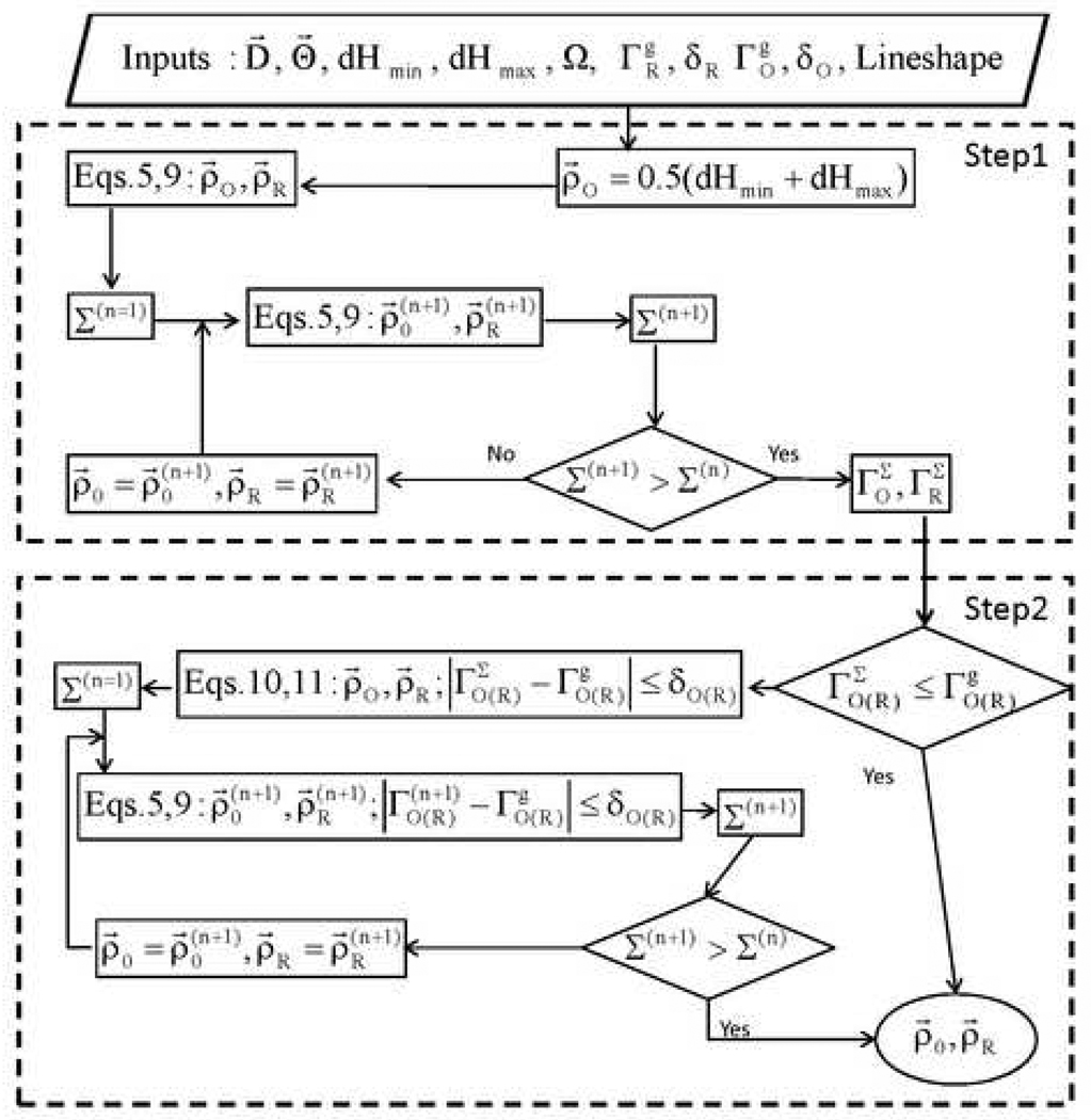
The goal of the algorithm is to find profiles ρ⃗_O and ρ⃗_R that minimize discrepancy with the data within the constraints of the regularization terms. Available a priori data can be used to specify the expected smoothness and thereby define ${\mathrm{\Gamma }}_{\mathrm{R}}^{\mathrm{g}}\text{ and }{\mathrm{\Gamma }}_{\mathrm{O}}^{\mathrm{g}}$, where g indicates goal. Experience with in vivo imaging is likely to produce reasonable estimates of these parameters for particular types of tissues. Profiles can then be sought that are within the limits: $\left|\Vert {\mathrm{L}}_{\mathrm{O}}{\overrightarrow{\mathrm{\rho }}}_{\mathrm{O}}\Vert -{\mathrm{\Gamma }}_{\mathrm{O}}^{\mathrm{g}}\right|\le {\mathrm{\delta }}_{\mathrm{O}}\text{ and }\left|\Vert {\mathrm{L}}_{\mathrm{R}}{\overrightarrow{\mathrm{\rho }}}_{\mathrm{R}}\Vert -{\mathrm{\Gamma }}_{\mathrm{R}}^{\mathrm{g}}\right|\mathrm{\le }{\mathrm{\delta }}_{\mathrm{R}}$. To reach the goal a large-scale non-linear optimization problem has to be solved. To find the global minimum is a complicated and time-consuming task. It suffices to obtain a solution with an error function that is close enough to the global minimum in a relatively short time. It was found empirically that more robust results were obtained if the search strategy was divided into two steps. These steps are described in the text below and shown in the flowchart representation of the algorithm (Figure 1).

Figure 1.

Flowchart for the regularized optimization (RO) algorithm. Input parameters are: experimental projections D⃗ ; angles Θ⃗ at which projections were measured; goals of regularization terms: ${\mathrm{\Gamma }}_{\mathrm{R}}^{\mathrm{g}},{\mathrm{\Gamma }}_{\mathrm{O}}^{\mathrm{g}}$ with error limits: δ_R, δ_O; expected lower and upper limits for linewidths dH_min and dH_max; positions in the sample with significant radical concentration, Ω; and the lineshape description. The goal of RO is to find the profiles ρ⃗_O and ρ⃗_R that minimize discrepancy with the data provided that $\left|\Vert {\mathrm{L}}_{\mathrm{O}}{\overrightarrow{\mathrm{\rho }}}_{\mathrm{O}}\Vert -{\mathrm{\Gamma }}_{\mathrm{O}}^{\mathrm{g}}\right|\le {\mathrm{\delta }}_{\mathrm{O}}\text{ and }\left|\Vert {\mathrm{L}}_{\mathrm{R}}{\overrightarrow{\mathrm{\rho }}}_{\mathrm{R}}\Vert -{\mathrm{\Gamma }}_{\mathrm{R}}^{\mathrm{g}}\right|\le {\mathrm{\delta }}_{\mathrm{R}}$. The search strategy can be divided into two steps. In the first step the discrepancy error ∑ is minimized without keeping track of changes in smoothness of the profiles. When the lowest error is reached, the algorithm searches (step 2) for solutions that are smooth enough to match the criteria ${\mathrm{\Gamma }}_{\mathrm{R}}^{\mathrm{g}}\text{ and }{\mathrm{\Gamma }}_{\mathrm{O}}^{\mathrm{g}}$. At this step the discrepancy error may increase at the expense of smoothing of the profiles and improving the accuracy of ρ⃗_O and ρ⃗_R.

3.1 Intermediate profiles (Step 1 in Figure 1)

The first step is reconstruction of intermediate profiles. Because the oxygen profile is gradually updated starting from a guess profile (Eq. (10)), it is reasonable to begin iterations with ρ⃗_O = const. This could be the linewidth of the non-gradient spectrum or an estimate of the average value. If something is known about the O₂ distribution, use of a more accurate initial guess can reduce computational time significantly. In the limiting case where ρ⃗_O is known, only a single implementation of Eq. (6) would be required to reach the final goal. Regularization parameters λ_i are adjusted iteratively to reduce the error function Σ⁽ⁿ⁾, where n is the number of the current iteration, until the next iteration brings no further improvement, Σ⁽ⁿ⁺¹⁾ ~ Σ⁽ⁿ⁾. The intermediate profiles are designated as ${\overrightarrow{\mathrm{\rho }}}_{\mathrm{O}}^{\mathrm{\Sigma }}\text{ and }{\overrightarrow{\mathrm{\rho }}}_{\mathrm{R}}^{\mathrm{\Sigma }}$ and the corresponding intermediate values of the regularization terms are designated as ${\mathrm{\Gamma }}_{\mathrm{O}}^{\mathrm{\Sigma }}\text{ and }{\mathrm{\Gamma }}_{\mathrm{R}}^{\mathrm{\Sigma }}$. Two approaches can be taken to improve these intermediate profiles. (i) The values of λ_R and λ_O can be varied and the impact on the error function monitored, analogous to the L-curve implementation of the Tikhonov method. (ii) If a priori information is available to define the expected smoothness of the profiles, values of ${\mathrm{\Gamma }}_{\mathrm{O}}^{\mathrm{g}}\text{ and }{\mathrm{\Gamma }}_{\mathrm{R}}^{\mathrm{g}}$ can be defined as goals, within specified limits, and values of λ_R and λ_O can be adjusted iteratively to achieve these goals with minimum impact on the error function. The values of ${\mathrm{\Gamma }}_{\mathrm{O}}^{\mathrm{\Sigma }}\text{ and }{\mathrm{\Gamma }}_{\mathrm{R}}^{\mathrm{\Sigma }}$ are upper limits on ${\mathrm{\Gamma }}_{\mathrm{O}}^{\mathrm{g}}\text{ and }{\mathrm{\Gamma }}_{\mathrm{R}}^{\mathrm{g}}$. Option (ii) is examined in this report.

3.2 Searching for profiles with target values of ${\mathrm{\Gamma }}_{\mathrm{O}}^{\mathrm{g}}\text{ and }{\mathrm{\Gamma }}_{\mathrm{R}}^{\mathrm{g}}$ (step 2 in Figure 1)

In the second step the algorithm keeps track of the smoothness of the profiles as well as changes in the error function. Reconstruction of ρ⃗_O involves a series of iterations, so each profile evolves from the previous one. If ${\mathrm{\Gamma }}_{\mathrm{O}}^{\mathrm{\Sigma }}$ is much larger than ${\mathrm{\Gamma }}_{\mathrm{O}}^{\mathrm{g}}$, it may take many iterations of ρ⃗_O to reach this goal because it is difficult to jump from a very noisy profile to a smooth one. This process can be accelerated by smoothing ${\overrightarrow{\mathrm{\rho }}}_{\mathrm{O}}^{\mathrm{\Sigma }}$ to get closer to ${\mathrm{\Gamma }}_{\mathrm{O}}^{\mathrm{g}}$ and using the smoothed profile ${\overrightarrow{\mathrm{\rho }}}_{\mathrm{O}}^{\mathrm{s}}$ as the new starting point. The following approach to smoothing was used.

$${\overrightarrow{\mathrm{\rho }}}_{\mathrm{O}}^{\mathrm{s}}=\mathrm{\alpha }{\overrightarrow{\mathrm{\rho }}}_{\mathrm{O}}^{\mathrm{n}}+(1-\mathrm{\alpha }){\overrightarrow{\mathrm{\rho }}}_{\mathrm{O}}^{\mathrm{\Sigma }};\mathrm{\alpha }\in [0,1];\text{ with the goal that}\Vert {\mathrm{L}}_{\mathrm{O}}{\overrightarrow{\mathrm{\rho }}}_{\mathrm{O}}^{\mathrm{s}}\Vert ={\mathrm{\Gamma }}_{\mathrm{O}}^{\mathrm{g}},$$ (11)

where ${\overrightarrow{\mathrm{\rho }}}_{\mathrm{O}}^{\mathrm{n}}$ is the result of n^th order polynomial fitting of ${\overrightarrow{\mathrm{\rho }}}_{\mathrm{O}}^{\mathrm{\Sigma }}$. Parameter n is adjusted, so that $\Vert {\mathrm{L}}_{\mathrm{O}}{\overrightarrow{\mathrm{\rho }}}_{\mathrm{O}}^{\mathrm{n}}\Vert <{\mathrm{\Gamma }}_{\mathrm{O}}^{\mathrm{g}}<\Vert {\mathrm{L}}_{\mathrm{O}}{\overrightarrow{\mathrm{\rho }}}_{\mathrm{O}}^{\mathrm{\Sigma }}\Vert$. To estimate α one can rewrite Eq. (11) in the form:

$$\begin{array}{c}(\mathrm{\alpha }\overrightarrow{\mathrm{V}}+\overrightarrow{\mathrm{U}}●\mathrm{\alpha }\overrightarrow{\mathrm{V}}+\overrightarrow{\mathrm{U}})={\mathrm{\alpha }}^2\overrightarrow{\mathrm{V}}●\overrightarrow{\mathrm{V}}+2\mathrm{\alpha }\overrightarrow{\mathrm{V}}●\overrightarrow{\mathrm{U}}+\overrightarrow{\mathrm{U}}●\overrightarrow{\mathrm{U}};\hfill \\ \overrightarrow{\mathrm{V}}={\mathrm{L}}_{\mathrm{O}}({\overrightarrow{\mathrm{\rho }}}_{\mathrm{O}}^{\mathrm{n}}-{\overrightarrow{\mathrm{\rho }}}_{\mathrm{O}}^{\mathrm{\Sigma }});\overrightarrow{\mathrm{U}}={\mathrm{L}}_{\mathrm{O}}{\overrightarrow{\mathrm{\rho }}}_{\mathrm{O}}^{\mathrm{\Sigma }};\mathrm{\alpha }\in [0,1];\hfill \end{array}$$ (12)

where (x ● x) is the dot product of two vectors. Solution of quadratic equation (12) gives parameter α. Substitution of α into Eq. (11) gives profile ${\overrightarrow{\mathrm{\rho }}}_{\mathrm{O}}^{\mathrm{s}}$, which when substituted into Eq. (6) produces ${\overrightarrow{\mathrm{\rho }}}_{\mathrm{O}}^{\mathrm{s}}$ with the desired Γ_R. This process produces profiles with good, but not necessarily the best, agreement with the data and with ${\mathrm{\Gamma }}_{\mathrm{O}}^{\mathrm{g}}\text{ and }{\mathrm{\Gamma }}_{\mathrm{R}}^{\mathrm{g}}$. Starting from these profiles, the algorithm iteratively adjusts λ_O and λ_R (Eqn. (6) and (10)) to minimize the error function, while keeping the regularization terms within the intervals ${\mathrm{\Gamma }}_{\mathrm{O}}^{\mathrm{g}}\pm {\mathrm{\delta }}_{\mathrm{O}}\text{ and }{\mathrm{\Gamma }}_{\mathrm{R}}^{\mathrm{g}}\pm {\mathrm{\delta }}_{\mathrm{R}}$. When iteration fails to reduce error, the algorithm terminates.

4. Experimental

4.1 Sample preparation

Electrochemically-prepared x-LiPc was graciously provided by Prof. Harold M. Swartz (Dartmouth Medical School) [26]. Multiple small crystals were placed in three quartz 3-mm OD tubes with 0.5 mm wall thickness. The amounts of sample in the three tubes were different. One tube was extensively evacuated and then flame sealed. The samples in the other two tubes were equilibrated with a 2% O₂ in nitrogen gas mixture then flame sealed. The three tubes were arranged in a row with the evacuated sample in the middle. Thus the center-to-center distances between samples in adjacent tubes were 3 mm.

4.2 Spectroscopy

The EPR spectra of the LiPc in each of the 3 tubes that composed the phantom were measured separately. The full widths at half height of the LiPc signals were 49 mG in the absence of O₂ and 148 or 169 mG for the two tubes with ~2% O₂. For image reconstruction dH_max was set at 250 mG and dH_min was set at 38 mG. Similar limits were used for fitting of the spectral slices from the FBP image.

Projections were acquired by rapid triangular-scan EPR [27]. Since the LiPc lineshape has mirror symmetry, the number of experimental projections could be reduced by a factor of two, relative to what would be needed in a general case. Projections for a 2-D spectral-spatial image were measured at 8 equally-spaced angles ranging from 5.63° to 84.38° in the spectral-spatial plane [28], with no ‘missing’ projections. Magnetic field gradients varied from 0.07 to 7.38 G/cm. The widths of the scans were adjusted to include regions of interest in the gradient-broadened spectra and scan frequencies were set to give a constant scan rate of 11 kG/s. For each projection 2048 data points were recorded that encompass both up-field and down-field scans. Spectra were Fourier-deconvoluted to recover the slow-scan signals [27]. After deconvolution the up-field and down-field scans were combined to increase signal-to-noise by a factor of √2. After summation the number of points in each projection was reduced to 287 by averaging and interpolation to permit FBP image reconstruction with the standard iradon Matlab routine.

Data sets obtained by averaging each projection 9216 or 50 times are denoted as "lower-noise" and "higher-noise", respectively.

4.3 Construction of Comparison Profiles and Image

For comparison with the reconstructed profiles, expected profiles were calculated. The linewidth profile was calculated from the known dimensions of the tubes and linewidths measured from the individual tubes: 148, 49, 169 mG, respectively. It was assumed that within each tube the linewidths for all LiPc crystals were the same. To assist in the calculation of the expected spatial profile, a spectrum at a gradient of 9.9 G/cm was averaged 200,704 times. This gradient is large enough that the signals from the three tubes were separated. Deconvolution of each signal individually, with a Lorentzian line of appropriate width, gave an estimate of the experimentally determined radical profile, ${\overrightarrow{\mathrm{\rho }}}_{\mathrm{R}}^{\mathrm{e}}$. The spatial variation is not smooth because of the nonuniform distribution of small crystallites in the tubes. Based on the linewidths for LiPc in the 3 tubes measured separately, and the estimate of the radical distribution profile, an image was reconstructed for comparison with the images obtained by the RO and FBP methods.

These profiles were used to produce a-priori information for the RO algorithm. Since the oxygen concentration is constant within each tube, ${\overrightarrow{\mathrm{\rho }}}_{\mathrm{O}}^{\mathrm{e}}$ is expected to consist of three flat lines with ${\mathrm{\Gamma }}_{\mathrm{O}}^{\mathrm{e}}=0.\text{ The}{\mathrm{\Gamma }}_{\mathrm{R}}^{\mathrm{e}}$ value calculated from the experimental profile, ${\overrightarrow{\mathrm{\rho }}}_{\mathrm{R}}^{\mathrm{e}}$, was 0.06 cm⁻¹.

4.4 FBP algorithm implementation

Images were reconstructed by FBP on grids of 201 · 201 pixels using 287 data points per projection by means of the standard iradon Matlab routine with default Ran-Lak filter and linear interpolation. Each spectral slice in the 2D spatial-spectral image was fitted to a Lorentzian lineshape by means of the lsqnonlin Matlab routine for nonlinear least-squares curve fitting. Fitting was done only in the spatial regions that correspond to the interior volume of the tubes. Other regions of the spectral-spatial images were defined as zeros. Use of this a priori information reduced the ‘star-effect’ distortion, which decreased the misfit error between projections from the FBP image and the experimental data by a factor of two. The ridges that radiate out from the tube regions have noticeable intensity in spaces between the tubes, so fitting in these parts of the image give rise to false values for radical concentration. The array of best fit linewidths from the 201 spectral slices is ${\overrightarrow{\mathrm{\rho }}}_{\mathrm{O}}^{\text{FBP}}$ and the integrated intensities for spectral slices are ${\overrightarrow{\mathrm{\rho }}}_{\mathrm{R}}^{\text{FBP}}$. Computations were done on a 3 GHz Pentium PC. The time needed for FBP reconstruction was about 0.2 seconds and the time required for non-linear least-squares fitting of the slices was about 7 seconds.

If the differences between projections at successive angles are not too large, images obtained by FBP can be improved by interpolation [29–31]. Since these procedures can also introduce artefacts, the comparison FBP images were reconstructed without interpolation.

4.5 RO algorithm implementation

The RO algorithm was implemented in Matlab. To speed up execution, matrix operations were used wherever possible. However, the algorithm has not been optimized, and rewriting some routines in C would make execution faster. The outputs of RO for this one-dimensional spatial case are ρ⃗_Oand ρ⃗_R. There is no need for an intermediate spectral-spatial image to be reconstructed. Values of ρ⃗_O and ρ⃗_R were calculated only in the regions where radical concentration was not zero. Regularization parameters were varied in very broad intervals λ_R=10⁻⁵–10⁵ and λ_O=(10⁻⁸–10²) to cover both lower and higher-noise datasets. For routine measurements of images with similar signal-to-noise ratios, this range can be narrowed to decrease computational time. For both datasets the algorithm worked to find values of Γ_i with ±3% accuracy. The initial guess ρ⃗_O for the first iteration was a constant 144 mG, which is the average of dH_min and dH_max. The average computational time, based on reconstruction of 182 images for various Γ_i values, was 4.5± 0.2 seconds for the projections with higher signal-to-noise ratio and 3.9±0.5 for the higher-noise dataset.

5. Results

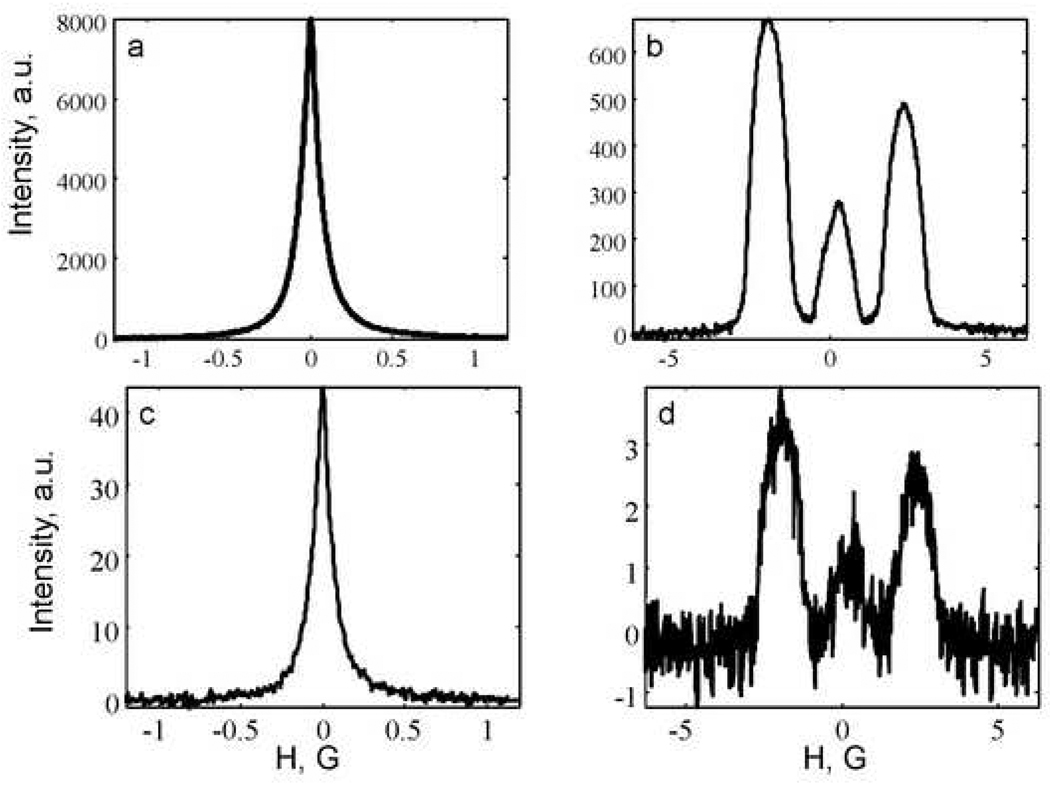
The RO algorithm was tested with two sets of projections with higher and lower noise levels, obtained by rapid-scan EPR at 250 MHz [27, 32]. Sample spectra obtained with gradients of 0.07 and 7.38 G/cm, respectively are shown in Fig. 2. For the higher noise data set the signal-to-noise (SNR) decreased from about 100 to 10 as the gradient was increased from 0.07 to 7.38 G/cm. The SNR was calculated as the amplitude of the most intense peak in the spectrum divided by the standard deviation of the noise in a baseline region. For the lower-noise data set the SNR decreased from about 1000 to 100, for the same increase in gradient. In both cases the impact of the gradient on signal-to-noise was much less than the quadratic dependence that would have been observed if the traditional first-derivative signals had been recorded [27].

Figure 2.

Examples of deconvolved rapid scan spectra recorded with two magnetic field gradients: 0.07 (parts a and c) and 7.38 G/cm (parts b and d). Spectra in parts a and b were averaged 9216 times (lower-noise data) and the spectra in parts c and d were averaged 50 times (higher-noise data).

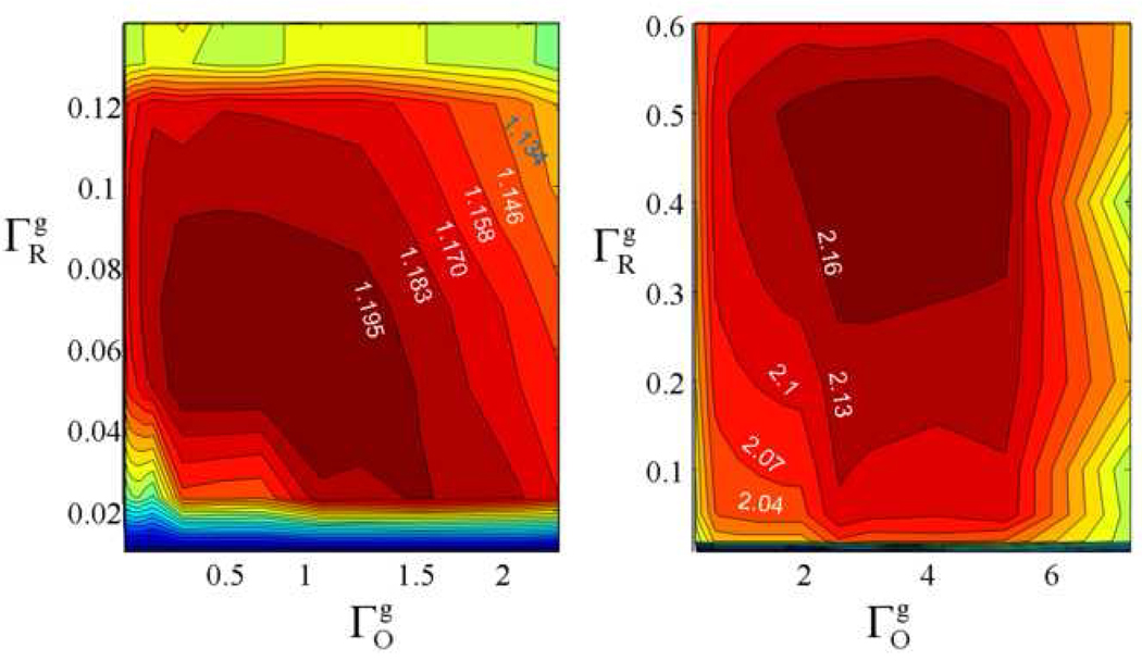
The error functions, Σ_RO, for profiles reconstructed by RO for various combinations of ${\mathrm{\Gamma }}_{\mathrm{R}}^{\mathrm{g}}\text{ and }{\mathrm{\Gamma }}_{\mathrm{O}}^{\mathrm{g}}$ were compared with Σ_FBP for images reconstructed by FBP. Sections of contour plots of the improvement ratio

$$\mathrm{\chi }({\mathrm{\Gamma }}_{\mathrm{R}}^{\mathrm{g}},{\mathrm{\Gamma }}_{\mathrm{O}}^{\mathrm{g}})=\frac{{\mathrm{\Sigma }}_{\text{FBP}}}{{\mathrm{\Sigma }}_{\text{RO}}}$$ (13)

as a function ${\mathrm{\Gamma }}_{\mathrm{R}}^{\mathrm{g}}\text{ and }{\mathrm{\Gamma }}_{\mathrm{O}}^{\mathrm{g}}$ are shown in Fig. 3. For each data set Σ_FBP is a constant, so the largest value of χ corresponds to the minimum error for RO reconstruction. If the experimental projections were exact Radon transforms of the spectral-spatial representation of the sample, the best match between the experimental data and ρ⃗_i would be found for Γ_R = 0.06 and Γ_O= 0, which was estimated from the phantom. In reality there is distortion by random noise and other hardware imperfections. For the low-noise data (Fig. 3a) the region with minimum error corresponds to Γ_R ~ 0.06, as expected from the phantom, but Γ_O is larger than for the phantom which is attributed to distortions in the data. For the higher-noise data (Fig. 3b) the region with minimum error occurs for Γ_R ~ 0.4 and Γ_O ~ 3.5. The larger values of Γ_O and Γ_R that minimize the error in Fig. 3b are attributed to the impact of noise in the data, which decreases the smoothness of the profiles. When the error function is used as the criterion for the "best" profiles, noise is incorporated into the profiles. Thus, the "best" match with the data may not be the "best" representation of the object. Based on the knowledge of the phantom it is possible to smooth the profiles from the noisy data to approach the values of Γ_R and Γ_O that are known for the phantom, and thereby obtain more accurate profiles, even though the error function is larger.

Figure 3.

Contour plots of the improvement in the error function for images reconstructed by RO relative to that for images reconstructed by FBP, χ(Γ_R, Γ_O), as a function of the regularization parameters Γ_R and Γ_O for the (a) lower-noise and (b) higher-noise data sets.

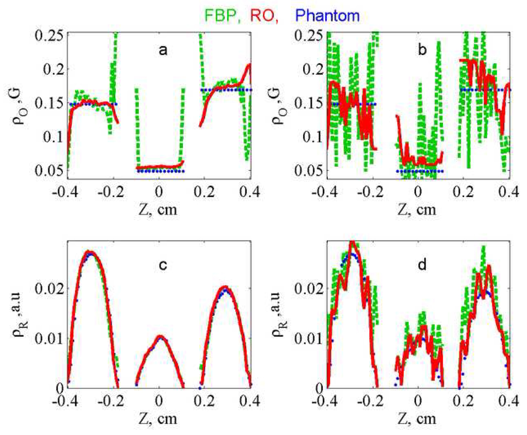
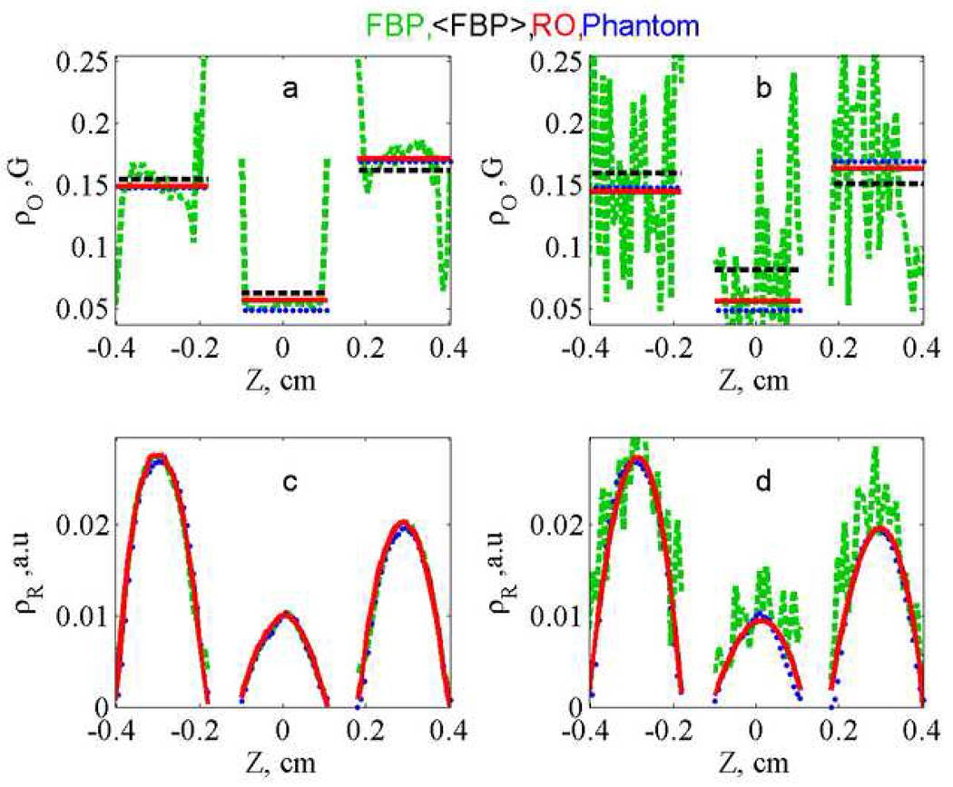
Additional insight concerning the algorithm can be obtained by comparing profiles calculated by RO and FBP. The intermediate profiles ${\overrightarrow{\mathrm{\rho }}}_{\mathrm{O}}^{\mathrm{\Sigma }}\text{ and }{\overrightarrow{\mathrm{\rho }}}_{\mathrm{R}}^{\mathrm{\Sigma }}$ obtained by minimizing the error function are compared with the profiles for the phantom and the slices from the FBP image in Fig. 4. For the lower-noise data (Fig. 4a) the oxygen profiles obtained by RO are smoother than those obtained by FBP, and both are in good agreement with the phantom. For the higher-noise data (Fig. 4b and 4d) the profiles are all noisier, but the RO profiles are smoother than those obtained by FBP. The improvement that can be obtained by imposing known information about the profiles is shown in Fig. 5, where the regularization terms were set equal to the known values for the phantom, Γ_O = 0.0 and Γ_R = 0.06. For comparison the mean values of the oxygen profiles, within a given tube, were calculated from the FBP profiles. For the lower-noise data (Fig. 5a and 5c) the average values from the FBP profiles and RO profiles are very similar. However, for the higher-noise data (Fig. 5b and 5d) the advantages of RO are evident, especially for the spatial profile. Even if the FBP profiles were smoothed, it would be difficult to accurately define the distribution of radicals.

Figure 4.

Comparison of (a,b) ρ⃗_O (linewidths that reflect oxygen concentration) and ρ⃗_R (c,d) radical concentrations. Profiles obtained from lower-noise (a,c) and higher-noise (b, d) data sets by FBP (green, dashed) and RO intermediate image (red, solid) are compared with the expected profile (blue, dotted).

Figure 5.

Comparison of (a,b) ρ⃗_O (linewidths that reflect oxygen concentration) and ρ⃗_R (c,d) radical concentrations. Profiles obtained from lower-noise (a,c) and higher-noise (b, d) data sets by FBP (green, dashed) and RO image (red, solid) calculated with Γ_O= 0 , Γ_R=0.06, are compared with the expected profile (blue, dotted). The light-blue solid lines show the mean linewidths in the three tubes obtained from FBP profile.

The intermediate profiles and profiles after use of the smoothing goals are compared quantitatively in Table 1. Application of the goal constraints reduces the improvement factor χ to a greater extent for the higher-noise data than for the lower-noise data. The decrease in χ is attributed to smoothing that causes an increase in the RO error function. The discrepancies between the phantom and profiles obtained by RO or FBP are calculated using equation (14).

$${\mathrm{\xi }}_{\mathrm{i}}=\frac{\Vert {\overrightarrow{\mathrm{\rho }}}_{\text{phantom}}-{\overrightarrow{\mathrm{\rho }}}_{\text{FBP}}\Vert }{\Vert {\overrightarrow{\mathrm{\rho }}}_{\text{phantom}}-{\overrightarrow{\mathrm{\rho }}}_{\text{RO}}\Vert }\mathrm{i}=\mathrm{R}\text{ or }\mathrm{O}$$ (14)

where in both numerator and denominator the discrepancies between the phantom and the reconstructed profiles are calculated. For each of the cases examined, the profiles obtained by RO are in better agreement with the phantom than ones obtained by FBP, especially for the noisy data. The values in Table 1 show that application of regularization constraints to the intermediate profiles increases discrepancy error with the data but, at the same time, improves the resemblance of the calculated profiles with the phantom. The one exception is that the constraints do not improve the spatial profile for the low-noise data. In that case the spatial profile obtained for the intermediate profiles, before the smoothness constraints, may be more precise than the estimate of the spatial profile for the phantom. That estimate was obtained by deconvolution of a single high gradient projection with different lineshapes for individual tubes. Uncertainties in the data and the deconvolution filter impact the calculation of ${\mathrm{\Gamma }}_{\mathrm{O}}^{\mathrm{g}}$.

Table 1.

Comparison of intermediate profiles with images after application of target parameters

Data	profiles	χ	ξR	ξO
Higher-noise	intermediate	2.2	1.8	2.11
Higher-noise	${\mathrm{\Gamma }}_{\mathrm{O}}^{\mathrm{g}}=0.0\text{ and }{\mathrm{\Gamma }}_{\mathrm{R}}^{\mathrm{g}}=0.06.$	1.95	4.07	7.38 (2.3)a
Lower-noise	intermediate	1.19	1.47	2.24
Lower-noise	${\mathrm{\Gamma }}_{\mathrm{O}}^{\mathrm{g}}=0.0\text{ and }{\mathrm{\Gamma }}_{\mathrm{R}}^{\mathrm{g}}=0.06$	1.16	1.34	5.86 (1.4)a

^aValues in parentheses are calculated from the FBP image in which the oxygen profiles were the averages of values for each tube (Fig. 5).

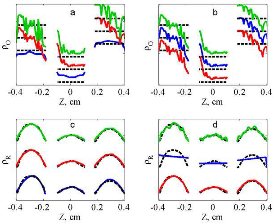
The changes in the profiles obtained from the higher-noise data that occur when the regularization terms are varied are shown in Fig. 6. As ${\mathrm{\Gamma }}_{\mathrm{O}}^{\mathrm{g}}$ is decreased from 2.1 to 1.1 and 0.11 the oxygen profile becomes smoother (Fig. 6a,c). Similarly as ${\mathrm{\Gamma }}_{\mathrm{R}}^{\mathrm{g}}$ is decreased from 0.41 to 0.06 and 0.005 the radical profile becomes smoother (Fig. 6b,d). If ${\mathrm{\Gamma }}_{\mathrm{i}}^{\mathrm{g}}$ is too large, excess noise is retained in the profile, but if ${\mathrm{\Gamma }}_{\mathrm{i}}^{\mathrm{g}}$ is too small then the profile is excessively smoothed. A-priori knowledge of appropriate values of regularization terms can be of great importance to reveal accurate profiles calculated from noisy experimental projections.

Figure 6.

Impact of Γ_R and Γ_O on radical and linewidth profiles for the lower noise data set. (a,c) varying Γ_O = 0.11 (lower, blue traces), 1.1 (middle, red traces), and 2.1 G/cm (top, green traces) with constant Γ_R = 0.06 and (b,d) varying Γ_R = 0.005 (lower, blue traces), 0.06 (middle, red traces), and 0.41 cm⁻¹ (top, green traces) with constant Γ_O = 1.1. Dashed black traces are the profiles in the phantom.

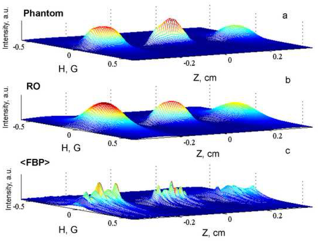
The images that correspond to the profiles obtained by RO from the higher-noise data with ${\mathrm{\Gamma }}_{\mathrm{R}}^{\mathrm{g}}=0.06\text{ and }{\mathrm{\Gamma }}_{\mathrm{O}}^{\mathrm{g}}=0$ are shown in Fig. 7, compared with that of the phantom and the image reconstructed by FBP with fitting of spectral slices to a Lorentzian, and the constraint that the oxygen profile is constant within each tube. The image obtained by RO is in much better agreement with the phantom than the image obtained by FBP.

Figure 7.

Comparison of the images reconstructed by RO (Γ_O=0 and Γ_R=0.06) and FBP (with average linewidths in each tube and fitting of each slice to a Lorentzian) from the lower-noise dataset with the phantom image.

5. Outlook

Reconstruction of EPR images is an ill-posed problem. Infinite number of solutions can be found that fit the experimental data almost equally well. Additional information about the sample is needed to increase the accuracy of reconstruction. Smoothing of the data is one of the commonly used methods to increase the robustness of the solution, often at the expense of distortion of some sharp details in the image. One of the important features of the RO algorithm is that smoothing is applied to the results, so some sharp features in the image can be included if these are strongly supported by the data. Another advantage of the algorithm is that it provides the experimenter with a tool to incorporate any a-priori knowledge into reconstruction such as lineshape of radical, geometry of the sample, biological peculiarities of different tissues with respect to accessibility of radical penetration and oxygen distribution. For example, radicals may accumulate in the bladder of an imaged animal. It is very likely that both O₂ molecules and radicals are evenly distributed throughout the urine due to diffusion. Instead of hundreds of unknowns for this region, only two are needed. Incorporation of this information increases the accuracy of reconstruction and reduces computational time. The phantom that was used to test the RO algorithm does not demonstrate all the possibilities of the algorithm and we are looking forward to further development of this approach to more dimensions and real biological systems.

6. Summary

An algorithm has been developed and tested that permits inclusion of a variety of a priori information in a flexible way. The constraint of known lineshape is built into the algorithm. Any lineshape could be used that can be described by a linewidth and an amplitude parameter. The algorithm directly constructs spatial profiles of oxygen and radical concentrations which reduces the dimensionality of the problem. Additional a priori information can include constraints on minimum and maximum linewidths and constraints on the average smoothness of the oxygen and radical profiles independently. Unlike FBP, projections do not need to be equally spaced, which means that projections may be selected that optimize information about the sample. Smoothing is achieved by applying average constraints on the profiles, unlike the process in FBP that smooths experimental projections. Reconstruction with the RO algorithm is about as fast as FBP with fitting of spectral slices. The RO algorithm may be even more computationally efficient if radical-containing regions are smaller than the whole reconstruction volume, because the regions with negligible spin density can be efficiently excluded from the iterations. For data with poorer signal-to-noise, the profiles obtained with the RO algorithm are in better agreement with experimental data and at the same time the reconstructed profiles are smoother. Although the algorithm is described and implemented here for 2D images, the same approach could be used for 3D images. Implementation of the algorithm for 4D is challenging. It would require inverting a large N³×N³ matrix, where N is the number points in one dimension. Possible approaches include reconstruction of the 4D image as 3D slices, iteratively solving Eq. (6,10) for sub-regions, or using existing methods for large systems of algebraic equations [33].

References

- 1.Kuppusamy P, Zweier JL. Cardiac Applications of EPR Imaging. NMR in Biomedicine. 2004;17:226–239. doi: 10.1002/nbm.912. [DOI] [PubMed] [Google Scholar]
- 2.Matsumoto K, Yahiro T, Yamada K, Utsumi H. In Vivo EPR Spectroscopic Imaging for a Liposomal Drug Delivery System. Magn. Reson. Med. 2005;53:1158–1165. doi: 10.1002/mrm.20460. [DOI] [PubMed] [Google Scholar]
- 3.Hirayama A, Nagase S, Ueda A, Oteki T, Takada K, Obara M, Inoue K, Hirayama K, Koyama A. In Vivo Imaging of Oxidative Stress in Ischemia-Reperfusion Renal Injury Using Electron Paramagnetic Resonance. Am. J. Physiol. Renal Physiol. 2005;288:F597–F603. doi: 10.1152/ajprenal.00020.2004. [DOI] [PubMed] [Google Scholar]
- 4.Halpern HJ. Applications of in Vivo EPR Spectroscopy and Imaging in Cancer Research. Biol. Magn. Reson. 2003;18:469–482. [Google Scholar]
- 5.Subramanian S, Matsumoto K, Mitchell JB, Krishna MC. Radio Frequency Continuous-Wave and Time-Domain Epr Imaging and Overhauser-Enhanced Magnetic Resonance Imaging of Small Animals: Instrumental Developments and Comparison of Relative Merits for Functional Imaging. NMR Biomed. 2004;17:263–294. doi: 10.1002/nbm.897. [DOI] [PubMed] [Google Scholar]
- 6.Subczynski WK, Swartz HM. EPR Oximetry in Biological and Model Systems. Biol. Magn. Reson. 2005;23:229–282. [Google Scholar]
- 7.Stuttgart BG, Teubner, Chichester . Ill-Posedness and Accuracy, ch. 4. In: Natterer F, editor. The Mathematics of Computerized Tomography. New York: John Wiley and Sons; 1986. [Google Scholar]
- 8.Herman GT. Image Reconstruction from Projections: Fundamentals of Computerized Tomography. New York: Academic Press; 1980. [Google Scholar]
- 9.Hayner DA, Jenkins WK. The Missing Cone Problem in Computer Tomography. Adv. Comp. Vision and Image Proc. 1984;1:83–144. [Google Scholar]
- 10.Skilling J, Bryan RK. Maximum Entropy Image Reconstruction: General Algorithm. Mon. Not. Roy. Astr. Soc. 1984;211:111–124. [Google Scholar]
- 11.Tseitlin M, Dhami A, Eaton SS, Eaton GR. Comparison of Maximum Entropy and Filtered Back-Projection Methods to Reconstruct Rapid-Scan EPR Images. J. Magn. Res. 2007;184:157–168. doi: 10.1016/j.jmr.2006.09.027. [DOI] [PMC free article] [PubMed] [Google Scholar]
- 12.Tikhonov AN, Arsenin VY. Methods of Solving Ill-Posed Problems. Moscow: Nauka; 1986. [Google Scholar]
- 13.Morozov VA. Methods for Solving Incorrectly Posed Problems (English Translation by A. B. Aries) New York: Springer Verlag; 1984. [Google Scholar]
- 14.Engl HW, Gfrerer H. A Posterioiri Parameter Choice for General Regularization Methods for Solving Linear Ill-Posed Problems. Appl. Numer. Math. 1988;4:395–417. [Google Scholar]
- 15.Chiang Y-W, Borbat PP, Freed JH. Maximum Entropy: A Complement to Tikhonov Regularization for Determination of Pair Distance Distributions by Pulsed EPR. J. Magn. Reson. 2005;177:184–196. doi: 10.1016/j.jmr.2005.07.021. [DOI] [PubMed] [Google Scholar]
- 16.Chiang Y-W, Borbat PP, Freed JH. The Determination of Pair Distance Distributions by Pulsed ESR Using Tikhonov Regularization. J. Magn. Reson. 2005;172:279–295. doi: 10.1016/j.jmr.2004.10.012. [DOI] [PubMed] [Google Scholar]
- 17.Calamante F, Gadian DG, Connelly A. Correct Quantification of Bolus-Tracking MRI: Improved Characterization of the Tissue Residue Function Using Tikhonov Regularization. Magn. Reson. Med. 2003;50:1237–1247. doi: 10.1002/mrm.10643. [DOI] [PubMed] [Google Scholar]
- 18.Hansen PC. Analysis of Ill-Posed Problems by Means of the L-Curve. SIAM Rev. 1992;34:561–580. [Google Scholar]
- 19.Johnston PR, Gulrajani RM. Selecting the Corner in the L-Curve Approach to Tikhonov Regularization. IEEE Trans. Biomed. Engin. 2000;47:1293–1296. doi: 10.1109/10.867966. [DOI] [PubMed] [Google Scholar]
- 20.Iwama N, Yoshida H, Takimoto H, Shen Y, Takamura S, Tsukishima T. Phillips-Tikhonov Regularization of Plasma Image Reconstruction with the Generalized Cross Validation. Appl. Phys. Lett. 1989;54:502–504. [Google Scholar]
- 21.Golub G, Heath M, Wahaba G. Generalized Cross-Validation as a Method for Choosing a Good Ridge Parameter. Technometrics. 1979;21:215–223. [Google Scholar]
- 22.Yang WQ, Peng L. Image Reconstruction Algorithms for Electrical Capacitance Tomography. Meas. Sci. Tech. 2003;14:R1–R13. [Google Scholar]
- 23.Stillman AE, Levin DN, Yang DB, Marr RB, Lauterbur PC. Back Projection Reconstruction of Spectroscopic Nmr Images from Incomplete Sets of Projections. J. Magn. Reson. 1986;69:168–175. [Google Scholar]
- 24.Elas M, Ahn KH, Parasca A, Barth ED, Lee D, Haney C, Halpern HJ. Electron Paramagnetic Resonance Oxygen Images Correlate Spatially and Quantitatively with Oxylite Oxygen Measurements. Clin. Cancer Res. 2006;12:4209–4217. doi: 10.1158/1078-0432.CCR-05-0446. [DOI] [PubMed] [Google Scholar]
- 25.Som S, Potter LC, Ahmad R, Kuppusamy P. A Parametric Approach to Spectral-Spatial Imaging. J. Magn. Reson. 2007;186:1–10. doi: 10.1016/j.jmr.2006.12.018. [DOI] [PMC free article] [PubMed] [Google Scholar]
- 26.Grinberg VO, Smirnov AI, Grinberg OY, Grinberg SA, O'Hara JA, Swartz HM. Practical Conditions and Limitations for High Spatial Resolution of Multi-Site Epr Oximetry. Appl. Magn. Reson. 2005;28:69–78. [Google Scholar]
- 27.Joshi JP, Ballard JR, Rinard GA, Quine RW, Eaton GR. Rapid-Scan EPR with Triangular Scans and Fourier Deconvolution to Recover the Slow-Scan Spectrum. J. Magn. Reson. 2005;175:44–51. doi: 10.1016/j.jmr.2005.03.013. [DOI] [PubMed] [Google Scholar]
- 28.Eaton SS, Eaton GR. EPR Imaging. Spectroscopy (Duluth, MN, United States) 1986;1:32–35. [Google Scholar]
- 29.Weiss GH, Talbert AJ, Brooks RA. The Use of Phantom Views to Reduce CT Streaks Due to Insufficient Angular Sampling. Phys. Med. Biol. 1982;27:1151–1162. doi: 10.1088/0031-9155/27/9/005. [DOI] [PubMed] [Google Scholar]
- 30.Placidi G, Alecci M, Sotgiu A. Angular Space-Domain Interpolation for Filtered Back Projection Applied to Regular and Adaptively Measured Projections. J. Magn. Reson. B. 1996;110:75–79. [Google Scholar]
- 31.Ahn K-H, Halpern HJ. Comparison of Local and Global Angular Interpolation Applied to Spectral-Spatial EPR Image Reconstruction. Medical Physics. 2007;34:1047–1052. doi: 10.1118/1.2514090. [DOI] [PubMed] [Google Scholar]
- 32.Stoner JW, Szymanski D, Eaton SS, Quine RW, Rinard GA, Eaton GR. Direct-Detected Rapid-Scan EPR at 250 Mhz. J. Magn. Res. 2004;170:127–135. doi: 10.1016/j.jmr.2004.06.008. [DOI] [PubMed] [Google Scholar]
- 33.Matej S, Fessler JA, Kazantsev IG. Iterative Tomographic Image Reconstruction Using Fourier-Based Forward and Back- Projectors. IEEE Trans. Med. Imag. 2004;23:401–412. doi: 10.1109/TMI.2004.824233. [DOI] [PubMed] [Google Scholar]