HOW DO SPATIAL AND ANGULAR RESOLUTION AFFECT BRAIN CONNECTIVITY MAPS FROM DIFFUSION MRI?

Abstract

Diffusion tensor imaging (DTI) is sensitive to the directionally- constrained flow of water, which diffuses preferentially along axons. Tractography programs may be used to infer matrices of connectivity (anatomical networks) between pairs of brain regions. Little is known about how these computed connectivity measures depend on the scans’ spatial and angular resolutions. To determine this, we scanned 8 young adults with DTI at 2.5 and 3 mm resolutions, and an additional subject at 4 resolutions between 2–4 mm. We computed 70×70 connectivity matrices, using whole-brain tractography to measure fiber density between all pairs of 70 cortical and subcortical regions. Spatial and angular resolution affected the computed connectivity for narrower tracts (internal capsule and cerebellum), but also for the corticospinal tract. Data resolution affected the apparent role of some key structures in cortical anatomic networks. Care is needed when comparing network data across studies, and interpreting apparent disagreements among findings.

1. INTRODUCTION

DTI and its variants (HARDI, DSI) are greatly advancing our understanding of neurological and psychiatric illness. DTI is widely used in international efforts to map brain connectivity in populations of thousands of subjects, such as the $30 million Human Connectome Project (www.humanconnectomeproject.org). Much of the effort to map brain networks has focused on DTI and its extensions, which can map axonal pathways and tracts in the living brain. Diffusion MRI is sensitive to the local direction and rate of water diffusion, at each location in the brain. Axonal pathways may be reconstructed using tractography methods to infer the most likely paths of tracts, based on tensor or higher-order (q-space) diffusion models [1]. Other methods exist to map functional connectivity, but the meaning of connectivity is different – in resting-state fMRI and MEG/EEG, temporal correlations are measured between signals at pairs of locations in the brain. These correlation matrices are then thresholded to identify network “hubs” important for functional synchronization of brain activity.

Diffusion MRI connectivity mapping has broad applications in neurology and psychiatry for understanding disrupted patterns of brain connections in Alzheimer’s disease, autism [2] and neurogenetic disorders of childhood, as well as sex differences and genetic effects on connectivity [3]. Much of the technical innovation focuses on q-space imaging, which enriches the information available on local directional and radial diffusion. The quest to improve the local diffusion model has led to elaborate q-space sampling schemes with large numbers of directional samples (HARDI), and/or multiple diffusion weightings (b-values) which are sensitive to non-monoexponential radial diffusion [4–6].

Several empirical and theoretical studies have modeled how signal to noise in DTI depends on the spatial and angular resolution of the scans [7–8]. Others have optimized the q-space sampling to boost SNR in clinically feasible scan times [9]. Much less attention has been devoted to understanding how brain networks, and patterns of recovered connections, depend on the spatial and angular resolution of the scans. Spatial resolution affects even the simplest measures derived from DTI, such as fractional anisotropy – the most widely used measure of brain integrity; in larger voxels, FA measures can be greatly reduced by partial volume effects. Here we scanned 9 young adults to monitor how different scanning protocols affect the recovery of maps of brain connectivity.

We hypothesized that both spatial and angular resolution would affect measures of cortical and subcortical connectivity. We were interested in the anatomical scope and extent of these effects. Empirical data on these questions will help to determine how well scan data may be pooled or compared in multi-site DTI studies; many of these are now being planned or are underway. Those designing DTI protocols may also be interested to know how comparable their brain connectivity maps are likely to be, relative to independently collected data from other imaging centers.

2. METHODS

2.1. Data description

Our first multi-resolution DTI dataset (called the “Mayo dataset”) was collected at the Mayo Clinic. 8 healthy subjects (age: 32.0 years ± 3.9 SD; 4 males) were scanned on a GE 3 Tesla brain MRI scanner with an 8-channel head coil. DWI data was collected using two protocols, summarized in Table 1.

Table 1.

Imaging protocols for the Mayo dataset

	Protocol 1 (P1)	Protocol 2 (P2)
Isotropic voxel size (mm)	3.0	2.5
Prescribed matrix	128 × 128	128 × 128
Number of slices	40	48
Number of DWI	48	37
Number of b0 images	4	4
TR (ms)	7750	9825
b-value (s/mm2)	1000	1000

For our second data set, a healthy male subject (32 years old) was scanned at multiple spatial resolutions (2×2×2, 2.5×2.5×2.5, 3×3×3 and 4×4×4 mm³) with axial DTI using the following acquisition parameters: TR=8000 ms, TE=83 ms, 128×128 matrix, 64 slices, b-value=1000 s/mm², one baseline (b₀) scan and 12 gradient directions. Although the number of diffusion directions for this second dataset is less than state-of-the-art (12), the large number of values of the spatial resolution makes it of interest.

2.2. Data processing

We first eddy-corrected all EPI images using FSL (http://fsl.fmrib.ox.ac.uk/fsl). Geometric distortions due to magnetic susceptibility were corrected using a simultaneously collected field map, using the FSL “Prelude and Fugue” function. Non-brain regions were removed from a T2-weighted image in the corrected DWI dataset using the bet function in FSL.

Depending on the number of the gradient directions in each dataset, we used two different models to analyze the preprocessed DWI. For the 12-direction data, the standard diffusion tensor was fitted using the Diffusion Toolkit (http://trackvis.org/dtk/). More gradient directions were collected for the Mayo datasets (Table 1), so the orientation distribution function (ODF) for water diffusion was reconstructed voxelwise using the recently proposed Constant Solid Angle formula (CSA-ODF; Aganj et al., 2010) with 4^th-order spherical harmonics (SH):

$$\mathit{ODF}(\widehat{u})=\frac{1}{4\pi }+\frac{1}{16{\pi }^2}\mathit{FRT}\{{\nabla }_b^{2}ln(-ln\stackrel{\sim }{E}(\widehat{u}))\}$$ (1)

Here û is the arbitrary unit vector. Ẽ (û) := S(û)/S₀, where S(û) is the diffusion signal, and S₀ is the non diffusion-weighted signal (from the b₀ scans). ${\nabla }_{\text{b}}^2$ is the Laplace-Beltrami operator and FRT is the Funk-Radon transform (Funk, 1916). ODFs were reconstructed using 642 point samples, from a recursively subdivided icosahedral approximation of the unit sphere.

2.3. White matter connectivity

50 white matter (WM) regions of interest (ROIs; Table 2) were generated based on the ICBM young adult DTI-81 atlas (http://www.loni.ucla.edu/ICBM/). ROIs were transformed into our datasets’ native coordinate space using 9-parameter linear registration. Using FSL-FLIRT, we registered the atlas T2-weighted image to the b₀ image of each individual dataset to obtain a transformation matrix. This was applied to all atlas WM ROIs to map them onto the target datasets.

Table 2.

50 white matter labels, used as the basis to compute 50×50 connectivity matrices.

1	Middle cerebellar peduncle	4	Body of corpus callosum
2	Pontine crossing tract	5	Splenium of corpus callosum
3	Genu of corpus callosum	6	Fornix
7–8	Corticospinal tract*	9–10	Medial lemniscus*
11–12	Inferior cerebellar peduncle*	13–14	Superior cerebellar peduncle*
15–16	Cerebral peduncle*	17–18	Anterior limb of internal capsule*
19–20	Posterior limb of internal capsule*	21–22	Retrolenticular part of internal capsule*
23–24	Anterior corona radiata*	25–26	Superior corona radiata*
27–28	Posterior corona radiata*	29–30	Posterior thalamic radiation*
31–32	Sagittal stratum*	33–34	External capsule*
35–36	Cingulum (cingulate gyrus)*	37–38	Cingulum (hippocampus)*
39–40	Fornix (cres)/Stria terminalis*	41–42	Superior longitudinal fasciculus*
43–44	Superior fronto- occipital fasciculus*	45–46	Inferior fronto-occipital fasciculus*
47–48	Uncinate fasciculus*	49–50	Tapetum*

^*indicates this ROI appears in both hemispheres (odd number for right hemisphere and even number for left hemisphere).

White matter connectivity was then computed from a fast-marching based method [10]. Given a seed region, the generalized fast-marching (GFM) method evolves a front outward according to the alignment of underlying fiber distributions. The GFM algorithm accept ts any spherical measure of fiber orientation – such as conventional tensors or ODFs – these are normalized to unit mass and sampled in directions coinciding with the displacement vectors to each voxel in the 98-neighborhood of a voxel under consideration (Fig. 1). The 98-neighborhood consists of all neighbors in the dilated 3×3×3 volume, plus those in the 5×5×5 volume whose displacement vectors do not coincide with any of those in the smaller neighborhood; this expansion of the neighborhood beyond the closest 26 voxels reduces the discretization error. At each iteration, the GFM algorithm adds one voxel to the advancing front; we decide which voxel to include based on a speed function that accounts for anisotropy and collinearity of fiber orientations at the source and destination voxels (Eq. 2):

$$\text{v}(\text{x},\text{n})=\text{gf}(\text{x},{\text{u}}_{\text{n}})\text{f}({\text{x}}_{\text{n}},{\text{u}}_{\text{n}})+(1-\text{g})<{\text{u}}_{\text{n}},{\text{u}}_{\text{e}}{>}^2$$ (2)

where x is a voxel on the boundary of the front, x_n is its n-th neighbor just outside the front, g is the mean generalized fractional anisotropy (GFA) between x and x_n, u_n is the normalized displacement vector to the n-th neighbor, u_e is the entrance direction with which the front moved to include x, and f(x,u_n) indicates the fiber orientation probability in the n-th direction at voxel x. The two terms in this equation are weighted differentially by the generalized fractional anisotropy (GFA) – in highly anisotropic regions, fiber orientation information is more reliable and the first term takes precedence, as it quantifies fiber orientation collinearity. In low anisotropy areas, the second term is favored, which prefers that the front continue to move in its current direction. Given this velocity, the front arrival time at each neighbor is computed simply from Eq. 3:

$$\text{t}({\text{x}}_{\text{n}})=\text{t}(\text{x})+\frac{\left|\right|\text{x}-{\text{x}}_{\text{n}}\left|\right|}{\text{v}(\text{x},\text{n})}$$ (3)

Fig. 1.

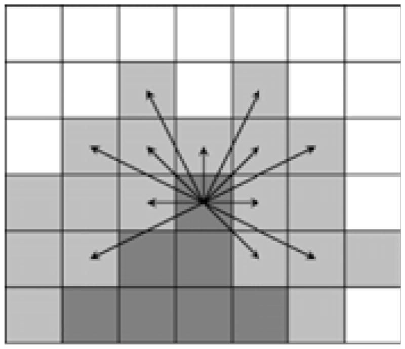
Front evolution in fast-marching tractography. One voxel from the band under consideration (light gray) is accepted into the advancing front (dark gray) at each iteration. Arrows indicate potential transitions from one voxel on the edge of the front. A speed function dictates which transition is made.

The voxel along the edge of the advancing front with the earliest arrival time is accepted into the front, and the neighbors of the newly-incorporated voxel are added to the list of potential transitions to consider in the next iteration. Marching continues in this manner until the front has evolved through the entire brain.

Connectivity is quantified by tracking a number of measures during the GFM evolution. The front arrival time is stored for each voxel along with the path distance taken to incorporate the voxel, the mean anisotropy along that path, the mean transition velocity of the front towards each voxel, and the minimum velocity step along the path to each voxel. Maps of all these attributes imply various features of “connectivity”, and are combined by standardizing the maps (subtracting the mean and dividing by the standard deviation across each subject’s map), performing principal component analysis (PCA), and extracting the projection of each voxel’s attributes onto the principal component vector. This score provides a robust “connectivity index” between WM ROIs.

2.4. Cortical connectivity

Cortical connectivity matrices were computed as in [3]. 35 cortical labels per hemisphere (Table 3) were automatically extracted from the same subjects’ T1-weighted structural MRI scans using FreeSurfer (http://surfer.nmr.mgh.harvard.edu/). As the software performs a linear registration, the resulting T1-weighted images and cortical models were aligned to the original T1 input image space and down-sampled to the space of the DWIs, using nearest neighbor interpolation (to avoid mixing of labels). To ensure tracts would intersect labeled cortical boundaries, labels were dilated with an isotropic box kernel of 5 voxels.

Table 3.

35 cortical labels per hemisphere were extracted, as the basis for our 70×70 cortical connectivity matrices.

1	Banks of the superior temporal sulcus
2	Caudal anterior cingulate	19	Pars orbitalis
3	Caudal middle frontal	20	Pars triangularis
4	Corpus callosum	21	Peri-calcarine
5	Cuneus	22	Postcentral
6	Entorhinal	23	Posterior cingulated
7	Fusiform	24	Pre-central
8	Inferior parietal	25	Precuneus
9	Inferior temporal	26	Rostral anterior cingulate
10	Isthmus of the cingulate	27	Rostral middle frontal
11	Lateral occipital	28	Superior frontal
12	Lateral orbitofrontal	29	Superior parietal
13	Lingual	30	Superior temporal
14	Medial orbitofrontal	31	Supra-marginal
15	Middle temporal	32	Frontal pole
16	Parahippocampal	33	Temporal pole
17	Paracentral	34	Transverse temporal
18	Pars opercularis	35	Insula

Fiber tracking was initiated by specifying three parameters: the threshold values for starting and stopping tracking, and the critical angle threshold for stopping tracking if the algorithm encounters a sharp turn in the fiber direction. Based on the diffusion tensor model, the Diffusion Toolkit (http://trackvis.org/dtk/) uses these parameters to generate 3D fiber tracts using the Fiber Assignment by Continuous Tracking (FACT) algorithm. With a brute-force reconstruction approach, we used all voxels in the volume as seed voxels to generate the fibers. After that, a spline filter was applied to each generated fiber, with units expressed in terms of the minimum voxel size of the dataset. After whole brain tractography, a 70×70 connectivity matrix was created. Each matrix element estimates the proportion of the total number of fibers, in that dataset, connecting each of the labels to the others.

3. RESULTS AND DISCUSSION

3.1. How does angular resolution affect measures of white matter connectivity?

We chose the P1 dataset (Table 1) for this test as it has the highest angular resolution (48 gradients). We downsampled the original dataset from 48 to k=47, 46… 16, 15 DWIs. Sub-sampling was based on maximizing the total angular distribution energy of the remaining set of k gradients, to optimize the uniformity of the spherical sampling (see [7]). We calculated white matter connectivity based on 4^th-order SH CSA-ODFs (Eq. 1) for each subsampled dataset as in Section 2.3. Then we assessed how angular resolution affected white matter connectivity. (This angular subsampling slightly overestimates the consistency achievable in scans of the same subject across independent scanning sessions). But, by subsampling the same dataset, we can isolate the effect of angular sampling and model it, with other sources of variance held constant. Fig. 2 shows the standard deviation (a measure of instability) of the connectivity matrix elements among the connectivity maps calculated from subset 15 to subset 48; this standard deviation was computed in each of the 8 subjects, and then averaged across all 8, to infer general patterns. As expected, some of the thinnest (narrowest) fiber tracts – the cerebellar ICP and SCP, and the internal capsules – were strongly affected by altering the angular resolution. Even some of the major pathways, including the apparent connections of the cortico-spinal tract with the ACR, ALIC and SFO were also quite severely influenced (red colors, Fig. 2).

Fig. 2. Angular resolution affects white matter connectivity measures.

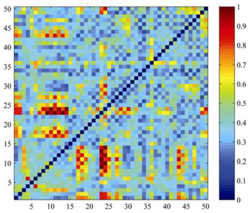
The names of the ROIs are listed in Table 2. In the red cells, varying the angular resolution of the scan affected the proportion of fibers apparently connecting the two regions of interest (on the x and y axes). Data show the standard deviation of the computed proportion of fibers.

3.2. Isolating the spatial resolution effect on apparent white matter connectivity

In general, changing the spatial resolution will also change the SNR for any DTI-derived measure. We chose the P2 dataset in Table 1 as the target, and gradually reduced its spatial resolution by downsampling its isotropic voxels of side 2.5 mm to 2.6, 2.7, …, 10 mm. Although other choices are possible, we chose linear interpolation to downsample the original P2 images to create each new image. For each downsampled subset, we calculated white matter connectivity based on 4^th-order SH CSA-ODFs. Fig. 3 shows the standard deviation of connectivity matrix elements across connectivity maps calculated at all voxel sizes in the range 2.5, 2.6 …10 mm, averaged across all eight subjects. The computed WM connectivity in all tracts and all regions is affected by partial volume effects. Greatest differences were found in the connections of the medial lemniscus, cerebellar peduncles, internal capsules, which are among the thinnest tracts.

Fig. 3. White matter connectivity measures depend on the spatial resolution of the scans.

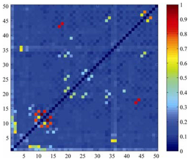
The names of the ROIs are listed in Table 2. Here the thinnest tracts – the internal capsules and cerebellar peduncles – are among those whose connectivity is least stable as the spatial resolution of the DTI scan is changed. The least stable tracts are shown in red.

3.3. Joint effect of spatial resolution and SNR on apparent white matter connectivity and cortical connectivity

As 4^th-order SH CSA-ODFs require at least 15 gradient directions to compute, we instead used the diffusion tensor model to evaluate white matter connectivity for the single subject scanned many times with only 12 gradient directions, but at multiple spatial resolutions. Fig. 4 shows the standard deviation of connectivity among connectivity maps calculated at 4 different isotropic spatial resolutions (2, 2.5, 3 and 4). These maps show more differences than those in Fig. 3, as signal averaging was used to boost the SNR for the scans with smaller voxels. By contrast, Fig. 3 is based on downsampling the exact same set of scans in 8 subjects, rather than performing new scans.

Fig. 4. White matter connectivity measures depend on the SNR and spatial resolution of the scans.

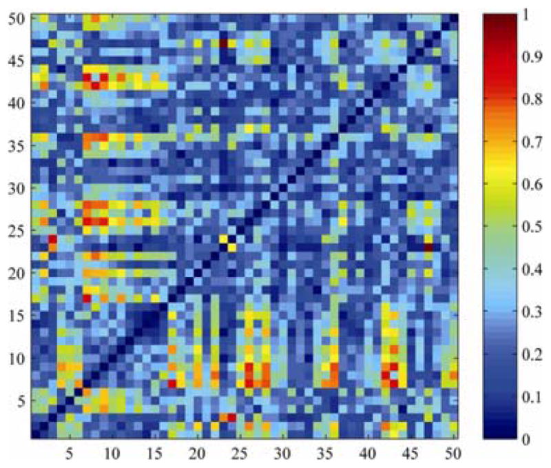
The names of the ROIs are listed in Table 2. Red matrix entries show connections that vary the most as spatial resolution was changed, in one subject scanned at 4 spatial resolutions. Many connections differ with spatial resolution; unlike Fig. 3, which downsampled the scan data without SNR varying.

Fig. 5 shows the standard deviation of elements in cortical connectivity matrices for 70 ROIs in the 12-direction dataset, at 4 different spatial resolutions. The computed pattern of cortical connectivity heavily depends on the spatial resolution, with less apparent connectivity in scans with large voxels. The cortical connection between parahippocampal and fusiform gyri, and between corresponding structures in the left and right hemispheres were most affected by spatial resolution.

Fig. 5.

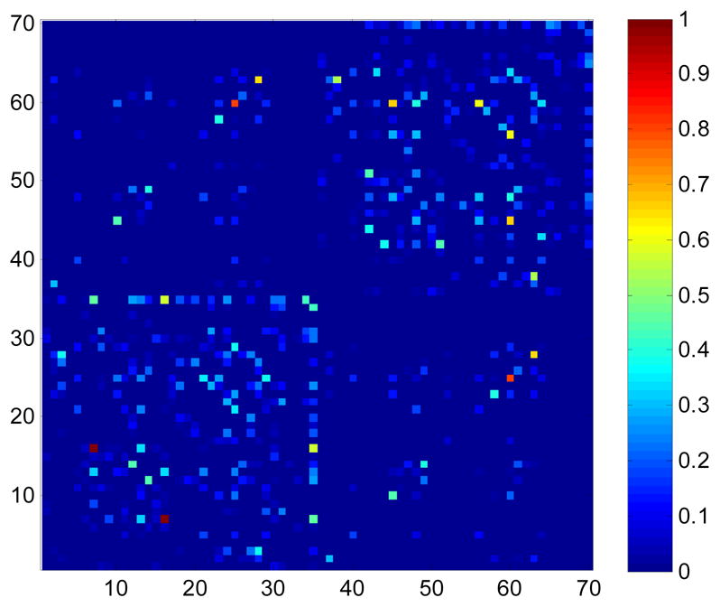
Cortical connectivity variation within a single subject scanned at 4 spatial resolutions. The names of the ROIs are listed in Table 3 (1–35, left hemisphere; 36–70, right hemisphere, e.g., ROIs 2 and 37 are the caudal anterior cingulate in the left and right hemispheres, respectively).

4. CONCLUSION

Overall, scans with larger voxels were prone to partial volume artifacts due to under-sampling, that causes a “loss” of some connections, especially for narrower tracts in the cerebellum and internal capsule. Differences were prominent throughout the brain. Care is needed when (1) interpreting anatomical connectivity patterns as objective measures of biological connectivity, (2) pooling data across scanners, and (3) comparing studies.

References

- 1.Aganj, et al. Reconstruction of the orientation distribution function in single and multiple shell q-ball imaging within constant solid angle. Magn Res Med. 2010;64(2):554–566. doi: 10.1002/mrm.22365. [DOI] [PMC free article] [PubMed] [Google Scholar]
- 2.Dennis, et al. Altered Structural Brain Connectivity in Healthy Carriers of the Autism Risk Gene, CNTNAP2. doi: 10.1089/brain.2011.0064. submitted to Brain Connectivity. [DOI] [PMC free article] [PubMed] [Google Scholar]
- 3.Jahanshad, et al. High angular resolution diffusion imaging (HARDI) tractography in 234 young adults reveals greater frontal lobe connectivity in women. ISBI; 2011; Chicago, Illinois, USA. 2011. pp. 939–943. [Google Scholar]
- 4.Assaf Y, Basser PJ. Composite hindered and restricted model of diffusion (CHARMED) MR imaging of the human brain. NeuroImage. 2005;27:48–58. doi: 10.1016/j.neuroimage.2005.03.042. [DOI] [PubMed] [Google Scholar]
- 5.Wedeen, et al. Mapping complex tissue architecture with diffusion spectrum magnetic resonance imaging. Magn Res Med. 2005;54(6):1377–1386. doi: 10.1002/mrm.20642. [DOI] [PubMed] [Google Scholar]
- 6.Zhan, et al. Differential Information Content in Staggered Multiple Shell HARDI Measured by the Tensor Distribution Function. ISBI; 2011; Chicago, Illinois, USA. 2011. pp. 305–309. [Google Scholar]
- 7.Zhan, et al. How does angular resolution affect diffusion imaging measures? NeuroImage. 2010;15;49(2):1357–71. doi: 10.1016/j.neuroimage.2009.09.057. [DOI] [PMC free article] [PubMed] [Google Scholar]
- 8.Landman, et al. Effects of diffusion weighting schemes on the reproducibility of DTI-derived fractional anisotropy, mean diffusivity, and principal eigenvector measurements at 1.5T. NeuroImage. 2007;36:1123–1138. doi: 10.1016/j.neuroimage.2007.02.056. [DOI] [PubMed] [Google Scholar]
- 9.Jahanshad, et al. Diffusion Tensor Imaging in Seven Minutes: Determining Trade-Offs Between Spatial and Directional Resolution. ISBI 2010; Rotterdam, The Netherlands. April 14–17; 2010. pp. 1161–1164. [Google Scholar]
- 10.Patel, et al. Fast-PC: A Method to Quantify Connectivity in DTI through Fast-Marching Tractography. Organization for Human Brain Mapping; Barcelona, Spain: Jun, 2010. [Google Scholar]