CRD: Fast Co-clustering on Large Datasets Utilizing Sampling-Based Matrix Decomposition

Abstract

The problem of simultaneously clustering columns and rows (co-clustering) arises in important applications, such as text data mining, microarray analysis, and recommendation system analysis. Compared with the classical clustering algorithms, co-clustering algorithms have been shown to be more effective in discovering hidden clustering structures in the data matrix. The complexity of previous co-clustering algorithms is usually O(m × n), where m and n are the numbers of rows and columns in the data matrix respectively. This limits their applicability to data matrices involving a large number of columns and rows. Moreover, some huge datasets can not be entirely held in main memory during co-clustering which violates the assumption made by the previous algorithms. In this paper, we propose a general framework for fast co-clustering large datasets, CRD. By utilizing recently developed sampling-based matrix decomposition methods, CRD achieves an execution time linear in m and n. Also, CRD does not require the whole data matrix be in the main memory. We conducted extensive experiments on both real and synthetic data. Compared with previous co-clustering algorithms, CRD achieves competitive accuracy but with much less computational cost.

1. INTRODUCTION

Clustering is a fundamental data mining problem with a wide variety of applications. It seeks good partitioning of the data points such that points in the same cluster are similar to each other and the points in different clusters are dissimilar. Many real-life applications involve large data matrices. For example, in text and web log analysis, the term-document data can be represented as contingency table. In biology domain, the gene expression data are organized in matrices with rows representing genes and columns representing experimental conditions. Recently there has been a growing research interest in developing co-clustering algorithms that simultaneously cluster both columns and rows of the data matrix. Co-clustering takes advantage of the duality between rows and columns to effectively deal with the high dimensional data. It has successful applications in gene expression data analysis [3] and text mining [5].

Many formulations of the co-clustering problem have been proposed, such as hierarchical model [12], bi-clustering model [3], pattern-based model [20] and so on. The partitioning-based model, which was first introduced in [12], has attracted much interest, because of the simplicity of the formalization and its close relationships to other well studied problems, such as spectral clustering and matrix decomposition [1, 5, 6, 8, 14, 15]. In this paper, we focus on the partitioning-based co-clustering formulation. Suppose that the data matrix D consists of m rows and n columns. Given input parameters k and l, the partitioning-based co-clustering algorithms aim to partition the rows of data matrix into k clusters and columns into l clusters to optimize certain objective functions measuring the quality of clustering results. Please refer to Section 2 for detailed discussion on recent development of co-clustering algorithms.

Although theoretically well studied and widely applied, existing co-clustering algorithms usually have time complexity in the order of m × n. For general data matrices, the information-theoretic co-clustering algorithm introduced in [5] takes O(t(k + l)mn) time to find the clustering results, where t is the number of iterations. Matrix-decomposition (such as nonnegative matrix factorization (NMF) [13]) based co-clustering methods [8, 15] have similar time complexity. In real-life applications, however, the numbers of rows and columns of the data matrices are usually large. For example, the term-document datasets may contain at least tens of thousands of articles and thousands of words [17]. The high throughput microarray techniques can monitor the expression values of tens of thousands of genes under hundreds to thousands of experimental conditions [16]. Such high time complexity limits the applicability of existing algorithms to these large datasets. Furthermore, these algorithms implicitly make the assumption that the whole data matrix is held in the main memory, since the original data matrix needs to be accessed constantly during the execution of these algorithms.

To address these limitations of existing work, in this paper, we propose a general co-clustering framework, CRD¹, for large datasets. This framework is based on recently developed sampling-based matrix decomposition method CUR [9, 18]. Unlike NMF based algorithms, the complexity of CRD algorithms is linear in m and n. Moreover, most of the operations in CRD involve only the sampled columns and rows. Therefore, we do not require the whole data matrix be in main memory. This is crucial for large datasets. CRD can be implemented using different algorithms such as k-means or information-theoretic co-clustering methods. We conduct extensive experiments on both synthetic and several well-known real-life datasets. The experimental results show that CRD can be orders of magnitude faster than previous information-theoretic methods and NMF based methods. At the same time, it achieves comparable accuracy to other methods.

2. RELATED WORK

Co-clustering has attracted much research interest in recent years. It simultaneously clusters columns and rows in the data matrix. In each iteration of the co-clustering procedure, rows(columns) are clustered based on their similarities in the column(row) clusters.

A notable early work is presented in [12] which adopts a splitting procedure to perform hierarchical row and column clustering on the data matrix. Recently, an information-theoretic algorithm specifically designed for contingency table is presented in [5]. The algorithm monotonically increases the preserved mutual information by intertwining row and column clusterings at successive stages. In [1], the authors further propose a more general co-clustering framework based on Bregman divergence, which includes squared Euclidean distance, KL-divergence, Itakura-Saito distance, etc., as special cases. Thus it is applicable to a wide range of data matrices. Given a general data matrix with n rows and m columns, the complexity of the information-theoretic co-clustering approaches is O(t(k + l)mn), where t is the number of iterations. This is because, in each iteration, the algorithm needs to compare each column or row with respect to the representative point of each cluster in the current clustering result. For sparse matrices, the algorithm can have O(t(k + l)|E|) complexity by efficient implementation, where |E| is the number of non-zero elements in the matrices.

Co-clustering is closely related to matrix decomposition. Singular value decomposition (SVD) [11] is perhaps the most well-known matrix decomposition method. The lower rank singular vector or eigenvector space provides a compact representation of the original space. Some research work [4, 7] clusters data points in the transformed space. However, since the factor matrices may contain negative values, it is hard to interpret the co-clustering results directly from SVD. Nonnegative matrix factorization (NMF) [13] imposes the constraint that the factor matrices contain only nonnegative values and has been successfully applied in document clustering [19]. In [15], the authors propose block value decomposition (BVD) for co-clustering. BVD generalizes the idea of NMF to factorize the original matrix into three nonnegative matrices, which provides intuitive interpretation of the co-clustering structure in the data matrix. The theoretic relationship between NMF and co-clustering is studied in [8]. It has been shown that the objective of k-means co-clustering and nonnegative matrix tri-factorizations with the orthogonal constraint are the same. A similar idea is also exploited in [14]. Similar to information-theoretic co-clustering, the time complexity of matrix decomposition based co-clustering methods usually is also in the order of m × n. For example, the complexity of BVD is O(t(k + l)mn) with t being the number of iterations. This is because updating the entries of the factor matrices usually involves multiplications of the data matrix.

Unlike PCA/SVD and NMF which generate new bases for the data space, recently developed matrix decomposition methods CUR [9] and CMD [18] sample columns and rows from the original data matrix to form factor matrices. Because of the random sampling procedure, these methods are non-deterministic. However, they can guarantee a provable bound on reconstruction error in probabilistic sense. CUR has been successfully applied in recommendation system [10].

3. PRELIMINARIES

In this section, we present notations that will be used in the paper and we provide formal definitions.

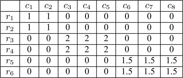
We denote the two-dimensional matrix(table) as $M,M\in {\mathbb{R}}^{m\times n}$. R = {r₁, r₂, ..., r_m} represents the set of row vectors of M, where r_i is the i^th row vector. C = {c₁, c₂, ..., c_n} represents the set of column vectors, where c_j is the j^th column vector. Thus, we have M = (c₁...c_n) = (r₁...r_m)^T. The element at the i^th row and j^th column is denoted by m_ij. Note that in this paper, we use bold font, such as c_i, to represent vector and use normal font, such as m_ij, to represent scalar. An example matrix consisting of 6 rows and 8 columns is shown in Figure 1.

Figure 1.

Example Matrix

A co-clustering of matrix M consists of a set of row clusters and column clusters. Let $\widehat{R}=\{{\widehat{r}}_1,{\widehat{r}}_2,\dots ,{\widehat{r}}_k\}$ denote the row cluster set and $\widehat{C}=\{{\widehat{c}}_1,{\widehat{c}}_2,\dots ,{\widehat{c}}_l\}$ denote the column cluster set. Each row of M belongs to one of the row clusters. This relationship can be considered as a many-to-one mapping from rows to row clusters, i.e., $\beta \left({\mathbf{r}}_{\mathbf{i}}\right)={\widehat{r}}_j,{\mathbf{r}}_{\mathbf{i}}\in R,{\widehat{r}}_j\in \widehat{R}$. The relationship between columns and column clusters is similar, i.e., $\theta \left({\mathbf{c}}_{\mathbf{i}}\right)={\widehat{c}}_j,{\mathbf{c}}_{\mathbf{i}}\in C,{\widehat{c}}_j\in \widehat{C}$.

Our CRD framework consists of two components.

1. Low rank matrix decomposition: The data matrix is decomposed using a subset of its rows and columns. The decomposition procedure must be fast and accurate.

2. Co-clustering on the subset of rows and columns: The selected rows and columns are co-clustered first. The cluster labels for the rest rows and columns are assigned based on those selected ones. In general, any co-clustering algorithm that optimizes its objective function by alternating the clustering of rows and columns can be used in CRD.

There may be many low rank decompositions for a given data matrix. However, not all of them are appropriate for co-clustering. Therefore, we provide definitions for qualified low rank row/column decompositions that can be used in CRD.

Definition 3.1. Low rank row decomposition: A low rank row decomposition of M approximates the original matrix using a subset of rows.

$$\tilde{M}=W_R\cdot M_R,where{W}_R\in {\mathbb{R}}^{m\times m^{\prime }},M_R\in {\mathbb{R}}^{m^{\prime }\times n}$$ (1)

W_R · M_R is a qualified low rank row decomposition of M if it satisfies the following constraints,

1. ${\Vert M-\tilde{M}\Vert }_F\le \epsilon {\Vert M\Vert }_F$, where ε < 1, is a user-specified approximation rate. ∥ · ∥_F represents the Frobenius matrix norm [11].

2. $M_R={\left({\mathbf{r}}_{u_1}{\mathbf{r}}_{u_2}\dots {\mathbf{r}}_{u_{m^{\prime }}}\right)}^T$, where $\left\{{\mathbf{r}}_{u_1}\dots {\mathbf{r}}_{u_{m^{\prime }}}\right\}\subset R$.

3. Given $M_R={\left({\mathbf{r}}_{u_1}{\mathbf{r}}_{u_2}\dots {\mathbf{r}}_{u_{m^{\prime }}}\right)}^T$, the corresponding rows in W_R have $\mid w_{u_{i}i}\mid >\mid w_{u_{i}j}\mid$, for all i ∈ {1, ..., m′} and j ∈ {1, ..., m′} − {i}.

Constraint 1 requires that matrix $\tilde{M}$ has small approximation error bounded by a user-specified threshold ε. The number of rows, m′, that need to be included in M_R can be calculated from ε and the rank of M. Constraint 2 ensures that each row vector in M_R is from M. And Constraint 3 ensures the correct mapping of the row cluster labels between selected rows and the rest rows. Details about the decomposition and its usage will be discussed in Sections 4 and 5 respectively.

Let W_R be represented by its row vectors, i.e., W_R = ( w₁ w₂ ... w_m )^T. Since $\tilde{M}=W_R\cdot M_R$, for each row vector in the approximation matrix $\tilde{M}$, we have,

$${\tilde{\mathbf{r}}}_i={({\mathbf{w}}_i^T\cdot M_R)}^T=\sum _{j=1}^{m^{\prime }}{w}_{ij}\cdot {\mathbf{r}}_{u_i}$$

Therefore, for each row ${\tilde{\mathbf{r}}}_i$, its corresponding row in W_R can be considered as a projection of ${\tilde{\mathbf{r}}}_i$ onto the sub-space formed by the rows in M_R.

The definition of low rank column decomposition of M is similar.

Definition 3.2 Low rank column decomposition: A low rank column decomposition of M approximates the original matrix using a subset of columns.

$$\tilde{M}=M_C\cdot W_C,where{M}_C\in {\mathbb{R}}^{m\times n^{\prime }},W_C\in {\mathbb{R}}^{n^{\prime }\times n}$$ (2)

M_C · W_C is a qualified low rank column decomposition of M if it satisfies the following constraints,

1. ${\Vert M-\tilde{M}\Vert }_F\le \epsilon {\Vert M\Vert }_F$, where ε < 1.

2. $M_C=\left({\mathbf{c}}_{v_1}{\mathbf{c}}_{v_2}\dots {\mathbf{c}}_{v_{n^{\prime }}}\right)$, where $\left\{{\mathbf{c}}_{v_1}\dots {\mathbf{c}}_{v_{n^{\prime }}}\right\}\subset C$.

3. Given $M_C=\left({\mathbf{c}}_{v_1}{\mathbf{c}}_{v_2}\dots {\mathbf{c}}_{v_{n^{\prime }}}\right)$, the corresponding columns in W_C have $\mid w_{i{v}_i}\mid >\mid w_{j{v}_i}\mid$, for all i ∈ {1, ..., n′} and j ∈ {1, ..., n′} − {i}.

For example, we can find a low rank row/column decomposition for the matrix in Figure 1. They are

$$\begin{array}{cc}\hfill W_R\cdot M_R& =\left(\begin{array}{ccc}\hfill 1\hfill & \hfill 0\hfill & \hfill 0\hfill \\ \hfill 1\hfill & \hfill 0\hfill & \hfill 0\hfill \\ \hfill 0\hfill & \hfill 1\hfill & \hfill 0\hfill \\ \hfill 0\hfill & \hfill 1\hfill & \hfill 0\hfill \\ \hfill 0\hfill & \hfill 0\hfill & \hfill 1\hfill \\ \hfill 0\hfill & \hfill 0\hfill & \hfill 1\hfill \end{array}\right)\cdot \left(\begin{array}{cccccccc}\hfill 1\hfill & \hfill 1\hfill & \hfill 0\hfill & \hfill 0\hfill & \hfill 0\hfill & \hfill 0\hfill & \hfill 0\hfill & \hfill 0\hfill \\ \hfill 0\hfill & \hfill 0\hfill & \hfill 2\hfill & \hfill 2\hfill & \hfill 2\hfill & \hfill 0\hfill & \hfill 0\hfill & \hfill 0\hfill \\ \hfill 0\hfill & \hfill 0\hfill & \hfill 0\hfill & \hfill 0\hfill & \hfill 0\hfill & \hfill 1.5\hfill & \hfill 1.5\hfill & \hfill 1.5\hfill \end{array}\right)\hfill \\ \hfill M_C\cdot W_C& =\left(\begin{array}{ccc}\hfill 1\hfill & \hfill 0\hfill & \hfill 0\hfill \\ \hfill 1\hfill & \hfill 0\hfill & \hfill 0\hfill \\ \hfill 0\hfill & \hfill 2\hfill & \hfill 0\hfill \\ \hfill 0\hfill & \hfill 2\hfill & \hfill 0\hfill \\ \hfill 0\hfill & \hfill 0\hfill & \hfill 1.5\hfill \\ \hfill 0\hfill & \hfill 0\hfill & \hfill 1.5\hfill \end{array}\right)\cdot \left(\begin{array}{cccccccc}\hfill 1\hfill & \hfill 1\hfill & \hfill 0\hfill & \hfill 0\hfill & \hfill 0\hfill & \hfill 0\hfill & \hfill 0\hfill & \hfill 0\hfill \\ \hfill 0\hfill & \hfill 0\hfill & \hfill 1\hfill & \hfill 1\hfill & \hfill 1\hfill & \hfill 0\hfill & \hfill 0\hfill & \hfill 0\hfill \\ \hfill 0\hfill & \hfill 0\hfill & \hfill 0\hfill & \hfill 0\hfill & \hfill 0\hfill & \hfill 1\hfill & \hfill 1\hfill & \hfill 1\hfill \end{array}\right)\hfill \end{array}$$

For both decompositions, we have ${\Vert M-\tilde{M}\Vert }_F=0$. Note that the rows in M_R and the columns in M_C are all selected from M. And both W_R and W_C satisfy Constraint 3 in our definition.

Using the 4 matrices, {M_R, W_R, M_C, W_C}, we want to find a co-clustering of M which is as good as the result obtained by running previous co-clustering algorithms on M directly.

4. LOW RANK ROW/COLUMN DECOMPOSITION

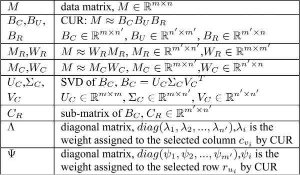
In our CRD framework, the row/column decomposition serves as a pre-processing step. Once M is decomposed into qualified matrices defined in Definitions 3.1 and 3.2, co-clustering algorithms will be applied on the decomposition matrices, {M_C, W_C, M_R, W_R}. In this section, we explain the details of the low rank row/column decomposition of the original matrix M. Before we start, we list a set of matrix notations that will be frequently used in this section in Figure 2.

Figure 2.

Notations for frequently used matrices

As defined in Definition 3.1, in low rank row decomposition, the matrix M is approximated by two decomposition matrices, M_R and W_R. M_R consists of a set of row vectors selected from M which establish a row sub-space. And W_R can be considered as a projection of all the row vectors in M onto the sub-space formed by rows in M_R.

We can use SVD to calculate W_R from M_R. First, we construct the orthogonal basis of M_R using SVD, i.e., M_R = U_RΣ_RV_R^T. Without loss of generality, we can assume that m′ < n, and let $V_R^{\prime }$ be a sub-matrix of V_R consisting of the first m′ row vectors in V_R(right eigenvectors). Then we can get a low rank approximation of M as

$$\tilde{M}=M\cdot V_R^{\prime }\cdot V_R^{\prime T}$$

Since we know that $V_R^{\prime }=M_R^T{U}_R{\Sigma }_R^{-1}$,

$$\begin{array}{cc}\hfill \tilde{M}& =M\cdot \left(M_R^T{U}_R{\Sigma }_R^{-1}\right)\cdot \left({\Sigma }_R^{-1}{U}_R^T{M}_R\right)\hfill \\ \hfill & =\left(M{M_R}^T{U}_R{\Sigma }_R^{-2}{U}_R^T\right)\cdot M_R\hfill \end{array}$$

Thus, $W_R=M{M_R}^T{U}_R{\Sigma }_R^{-2}{U}_R^T$.

In order to improve the efficiency of the entire algorithm, the approximate decomposition of M need to be calculated very efficiently. Most of the previous co-clustering algorithms have runtime complexity equal to or higher than O(t(k + l)mn) where k and l are the number of row/column clusters and t is the number of iterations. Therefore, the decomposition method we use need to have complexity lower than O(t(k + l)mn). When using SVD to calculate W_R, its time complexity is O(mnm′) where m′ is the number of selected rows. Though m′ << m, m′ is greater than or equal to k. Thus, it is inefficient to use SVD directly to calculate W_R.

In this paper, we use the CUR decomposition method proposed in [9, 18] to find qualified low rank row/column decompositions. The runtime complexity of CUR is mn + O((m + n)m′n′), in which mn is used to calculate the norm of each row/column vector. In fact, the norm of row and column vectors only need to be calculated once and can be stored with the matrix for further use. Besides mn, CUR has runtime O((m + n)m′n′) which is much smaller than O(t(k + l)mn).

The CUR method approximately decomposes M into three matrices, i.e.,

$$M\approx B_C\cdot B_U\cdot B_R$$

where $B_C\in {\mathbb{R}}^{m\times n^{\prime }}$ is a set of weighted columns selected from $M,B_R\in {\mathbb{R}}^{m^{\prime }\times n}$ is a set of weighted rows selected from M and $B_U\in {\mathbb{R}}^{n^{\prime }\times m^{\prime }}$. Rows and columns in B_C and B_R are randomly selected with probability in proportional to their norm. And B_U is calculated based on B_C and B_R.

If matrix M has rank equal to k, it is proven in [9] that

$${\Vert M-B_C\cdot B_U\cdot B_R\Vert }_F\le \epsilon {\Vert M\Vert }_F$$

holds with probability (1 − δ) if the numbers of selected columns and rows are at least

$$n^{\prime }=\frac{{(1+\sqrt{8log(1∕\delta )})}^2}{{\epsilon }^4},m^{\prime }=\frac{k}{{\delta }^2{\epsilon }^2}$$

Thus, if we use a small δ, with high probability, the CUR decomposition satisfies the first constraint on the approximation error between M and $\tilde{M}$ in Definitions 3.1 and 3.2. Details about the decomposition algorithm can be found in [9, 18].

Before we can use CUR to generate our low rank row/column decomposition, we have to make some changes in the method.

• B_C and B_R consist of weighted column and row vectors of M. While in our CRD algorithm, we need M_C and M_R consist of original row and column vectors of M.

• We only need to decompose M into two matrices while CUR gives us three. A simple multiplication of two of the matrices in {B_C, B_U, B_R} seems to be able to get W_R and W_C, i.e., W_R = B_C · B_U and W_C = B_U · B_R. However, we need to select rows and columns that do not violate Constraint 3 in Definitions 3.1 and 3.2. We will discuss it in the next section.

4.1 Generate Low Rank Row Decomposition Using CUR

First, we generate M_R from B_R. To approximate M, the three matrices used by CUR are,

$$\begin{array}{cc}\hfill & \tilde{M}=B_C\cdot B_U\cdot B_R\hfill \\ \hfill & =\left({\lambda }_1{\mathbf{c}}_{v_1}\dots {\lambda }_{n^{\prime }}{\mathbf{c}}_{v_{n^{\prime }}}\right)B_U{\left({\psi }_1{\mathbf{r}}_{u_1}\dots {\psi }_{m^{\prime }}{\mathbf{r}}_{u_{m^{\prime }}}\right)}^T\hfill \end{array}$$ (3)

where $B_C\in {\mathbb{R}}^{m\times n^{\prime }},B_U\in {\mathbb{R}}^{n^{\prime }\times m^{\prime }}$ and $B_R\in {\mathbb{R}}^{m^{\prime }\times n}$.

By multiplying each row vector in B_R with $\frac{1}{{\psi }_i}$, we get

$$M_R={\Psi }^{-1}{B}_R=\left(\begin{array}{ccc}\hfill 1∕{\psi }_1\hfill & \hfill 0\dots \hfill & \hfill 0\hfill \\ \hfill 0\dots \hfill & \hfill 1∕{\psi }_i\hfill & \hfill \dots 0\hfill \\ \hfill 0\dots \hfill & \hfill \dots 0\hfill & \hfill 1∕{\psi }_{m^{\prime }}\hfill \end{array}\right)B_R$$ (4)

Obviously, M_R in Equation 4 satisfies Constraint 2 in Definition 3.1.

Next, we generate a qualified W_R. By replacing B_R in Equation 3 with Ψ · M_R, we get

$$\tilde{M}=(B_C\cdot B_U\cdot \Psi )\cdot M_R$$ (5)

In CUR, given B_C and B_R,

$$B_U=V_C{\Sigma }_C^{-2}{V}_C^T{C}_R^{\prime T}$$ (6)

where V_C and Σ_C are singular vectors and singular values of B_C, i.e., $B_C=U_C{\Sigma }_C{V_C}^T.C_R^{\prime }$ consists of the {u₁, ..., u_m′}^th rows of B_C (the set of selected rows in B_R) and each row in $C_R^{\prime }$ is weighted by the corresponding ψ_i. To remove the weight ψ_i from each row of $C_R^{\prime }$, let

$$C_R={\Psi }^{-1}\cdot C_R^{\prime }$$ (7)

Using Equations 6 and 7, we have

$$B_C\cdot B_U\cdot \Psi =B_C{V}_C{\Sigma }_C^{-2}{V}_C^T{C}_R^T{\Psi }^2$$ (8)

Without loss of generality, we assume that n′ < m. Let $U_C^{\prime }$ be a sub-matrix of U_C which consists of the first n′ column vectors in U_C. We have

$$U_C^{\prime }=B_C\cdot V_C\cdot {{\Sigma }_C}^{-1}$$ (9)

By combing Equations 8 and 9, we have

$$B_C\cdot B_U\cdot \Psi =U_C^{\prime }\cdot U_{CR}^{\prime T}\cdot {\Psi }^2$$ (10)

where $U_{CR}^{\prime }$ consists of the {u₁, ..., u_m′}^th rows of $U_C^{\prime }$ which correspond to the selected rows in B_R.

Let W_R = B_C · B_U · Ψ², we have

$$W_R=B_C\cdot B_U\cdot \Psi =U_C^{\prime }\cdot U_{CR}^{\prime T}\cdot {\Psi }^2$$ (11)

Constraint 3 in Definition 3.1 only involves those rows in W_R which correspond to the selected rows in M_R(B_R). Let this sub-matrix of W_R be $W_R^{\prime }(W_R^{\prime }\in {\mathbb{R}}^{m^{\prime }\times m^{\prime }})$, we have

$$W_R^{\prime }=U_{CR}^{\prime }\cdot U_{CR}^{\prime T}\cdot {\Psi }^2$$ (12)

Let $U_{CR}^{\prime }={\left({{\mathbf{u}}^{\prime }}_1\dots {{\mathbf{u}}^{\prime }}_{m^{\prime }}\right)}^T.W_R^{\prime }$ satisfies Constraint 3 if and only if

$$\forall i,j\in \left\{1\dots m^{\prime }\right\},i\ne j,{\psi }_i^2\mid {{\mathbf{u}}^{\prime }}_i^T\cdot {{\mathbf{u}}^{\prime }}_i\mid >{\psi }_j^2\mid {{\mathbf{u}}^{\prime }}_i^T\cdot {{\mathbf{u}}^{\prime }}_j\mid$$ (13)

$U_{CR}^{\prime }$ is generated from $U_C^{\prime }$ according to the set of rows selected in B_R. In order to generate a qualified W_R, Equation 13 must be verified every time a new row is selected to be included in B_R.

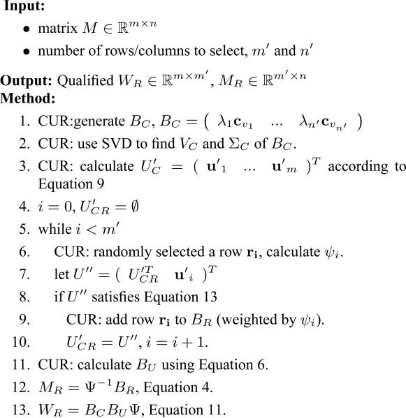
The algorithm to generate low rank row decomposition using CUR is shown in Figure 3.

Figure 3.

Generate Low Rank Row Decomposition Using CUR

In Figure 3, the steps labelled with CUR are the steps in the original CUR decomposition method. The remaining steps in Figure 3 are added to enforce the constraints defined on W_R and M_R. The qualification of W_R is ensured by the test in Step 8. A new row is added to B_R if and only if it does not violate Equation 13. The qualification of M_R is ensured in Step 12.

Note that the SVD operation in Step 2 is calculated by eigenvalue decomposition on $B_C^T{B}_C$ which is a small n′ × n′ matrix. $U_C^{\prime }$ is not calculated until Step 3.

4.2 Generate Low Rank Column Decomposition Using CUR

The algorithm in Figure 3 only ensures the qualification of W_R and M_R. Since the columns are randomly selected without any restriction in Step 1 in Figure 3, we cannot guarantee qualified M_C and W_C by simply letting M_C = B_CΛ⁻¹ and W_C = ΛB_UB_R.

However, if we transpose the original matrix M, exchange m′ and n′, and use them as input to the algorithm in Figure 3, we can get qualified M_C and W_C by letting

$$M_C=M_R^T,W_C=W_R^T$$ (14)

Therefore, in order to get a qualified low rank row/column decomposition, we need to run the algorithm in Figure 3 twice. In general, if the norms of row and column vectors of a data matrix have been calculated, our decomposition method will take O((m + n)m′n′) time to find a set of qualified matrices {M_R, W_R, M_C, W_C} where m′ and n′ are the numbers of selected rows and columns respectively. As we will show in the experiment section, the time used on finding the decomposition is minimal and can be neglected.

5. A GENERAL FRAMEWORK FOR CO-CLUSTERING USING ROW/COLUMN DECOMPOSITION: CRD

In order to perform co-clustering on large data matrix efficiently, in our CRD framework, the co-clustering is performed on the decomposition matrices instead of the original matrix M. It provides significant improvements in both space and time utilization.

As we discussed in Section 2, one type of co-clustering algorithms cluster the rows and columns of a data matrix alternatively in successive iterations. These algorithms include the Information Theoretic Co-clustering algorithm [5], the Bregman Co-clustering algorithm [1] and the Fully Automatic Cross-association algorithm in [2]. In each iteration, they either keep the row side clusters fixed and re-cluster the columns or keep the column side clusters fixed and re-cluster the rows. It is proved that this single side clustering (row or column) can guarantee the objective function on the co-clustering structure converge to a local minimum (maximum). We call it the Iterative Single Side Clustering approach.

Suppose that there are k row clusters, $\widehat{R}=\{{\widehat{r}}_1,\dots {\widehat{r}}_k\}$, and _l column clusters, $\widehat{C}=\{{\widehat{c}}_1,\dots {\widehat{c}}_k\}$. The co-clustering structure after the t^th iteration is represented by β^t and θ^t which map each row/column in the data matrix to a row/column cluster.

$$\begin{array}{cc}\hfill & \forall i\in \{1,\dots ,m\},{\beta }^t\left({\mathbf{r}}_{\mathbf{i}}\right)={\widehat{r}}_j,where{\widehat{r}}_j\in \widehat{R}\hfill \\ \hfill & \forall i\in \{1,\dots ,n\},{\theta }^t\left({\mathbf{c}}_{\mathbf{i}}\right)={\widehat{c}}_j,where{\widehat{c}}_j\in \widehat{C}\hfill \end{array}$$

An illustration of the Iterative Single Side Clustering approach is shown in Figure 4.

Figure 4.

Co-clustering using Iterative Single Side Clustering Approach

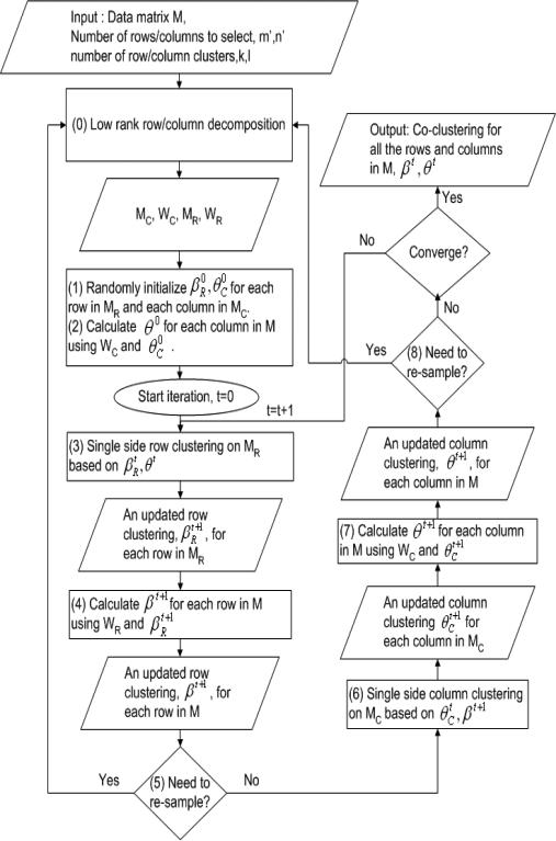
In this paper, we use this general approach as the co-clustering component in our CRD framework. In each iteration, instead of re-clustering all rows (or columns), we only re-cluster the selected rows in M_R or the selected columns in M_C. Then we assign cluster label to each row (or column) in M based on W_R (or W_C) and the cluster labels of the selected rows (columns).

Let the single-side clustering structure on the rows in M_R and the columns in M_C after the t^th iteration be

$$\begin{array}{cc}\hfill & \forall i\in \{1,\dots ,m^{\prime }\},{\beta }_R^t\left({\mathbf{r}}_{\mathbf{i}}\right)={\widehat{r}}_j,where{\widehat{r}}_j\in \widehat{R}\hfill \\ \hfill & \forall i\in \{1,\dots ,n^{\prime }\},{\theta }_C^t\left({\mathbf{c}}_{\mathbf{i}}\right)={\widehat{c}}_j,where{\widehat{c}}_j\in \widehat{C}\hfill \end{array}$$

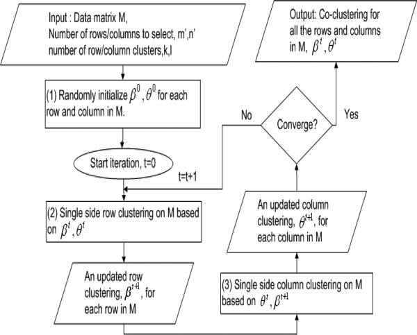
A detailed illustration of CRD is shown in Figure 5.

Figure 5.

Framework for Co-clustering using Decomposition: CRD

As we can see from Figures 5 and 4, Steps (1,2) in Figure 5 correspond to Step (1) in Figure 4, Steps (3,4) in Figure 5 correspond to Step (2) in Figure 4 and Steps (6,7) in Figure 5 correspond to Step (3) in Figure 4. Also, for those steps in the iteration loop, the steps in Figure 5 have much smaller time complexity than the corresponding steps in Figure 4. The comparison is shown in Table 1.

Table 1.

Complexity of Corresponding Steps in Co-clustering

		runtime		runtime
Figure 5	Steps(3,4)	O(km′n+m′m)	Steps(6,7)	O(ln′m+n′n)
Figure 4	Step(2)	O(kmn)	Step(3)	O(lmn)

In general, co-clustering using Iterative Single Side Clustering approach can have runtime complexity equal to (or larger than) O(t(k + l)mn) where t is the number of iterations. While CRD only uses O(t(km′n + ln′m + m′m + n′n)) plus the time used in matrix decomposition, O((m + n)m′n′), which is a one-time cost at the beginning. Since usually we have m′ << m and n′ << n, CRD is much faster.

The single side clustering in Steps (3) and (6) of CRD is exactly the same as the one in the Iterative Single Side Clustering approach. Details about the steps can be found in [5, 1]. We will discuss the two new steps, Steps (4,7) and Steps (5,8) in the following sections respectively.

5.1 Mapping Cluster Labels from Selected Rows /Columns to All Rows/Columns

In Steps (2), (4) and (7) of CRD, we calculate β (θ) for each row (column) in M using W_R (W_C) and β_R (θ_C). Since the procedure for calculating θ on columns is the same as that of calculating β on rows, we will only explain the calculation of β.

Using low rank row decomposition, M is approximated by W_R and M_R. Each row of W_R can be considered as a projection of the corresponding row of M onto the sub-space formed by the rows in M_R, i.e., there is a one-to-one relationship between a row of M and the corresponding row of W_R. Therefore, when we get the row cluster label for each row of M_R, we can use W_R to calculate the cluster label for each row of M.

Suppose that for each row ${\mathbf{r}}_{\mathbf{i}}^{\prime }$ of M_R, we have ${\beta }_R\left({\mathbf{r}}_{\mathbf{i}}^{\prime }\right)={\widehat{r}}_j,j\in \{1,\dots ,k\}$. For each row r_i of M, we calculate its label vector s_i = [s_i1, s_i2, ..., s_ik], in which

$$s_{ij}=max\left\{\mid w_{iz}\mid \mid {\beta }_R\left({\mathbf{r}}_{\mathbf{z}}^{\prime }\right)={\widehat{r}}_j\right\}$$ (15)

Then we have,

$$\beta \left({\mathbf{r}}_{\mathbf{i}}\right)=\left\{z\mid s_{iz}=max(s_{i1},\dots ,s_{ik})\right\}$$ (16)

Intuitively, s_ij is the correlation between row r_i and row cluster ${\widehat{r}}_j$. In Equation 16, r_i is assigned to the row cluster having the highest correlation.

Now we prove the following property.

Property 5.1. For each row ${\mathbf{r}}_{\mathbf{j}}^{\prime }$ of M_R and its corresponding row r_i of M, if we use Equations 15 and 16 to calculate β, we have

$$\beta \left({\mathbf{r}}_{\mathbf{i}}\right)={\beta }_R\left({\mathbf{r}}_{\mathbf{j}}^{\prime }\right)$$ (17)

Proof: According to Constraint 3 in Definition 3.1, we have |w_ij| > |w_iz|, z ∈ {1, ..., m′} − {j}. Assume that ${\beta }_R\left({\mathbf{r}}_{\mathbf{j}}^{\prime }\right)={\widehat{r}}_h$. When calculating s_i, we get

$$s_{ih}=max\left\{\mid w_{iz}\mid \mid {\beta }_R\left({\mathbf{r}}_{\mathbf{z}}^{\prime }\right)={\widehat{r}}_h\right\}=\mid w_{ij}\mid .$$

According to Equation 15, we know s_it ∈ {|w_i1|, ..., |w_im′|}, t ∈ {1, ..., k}. Thus we get

$$s_{ih}=max\left\{s_{it}\mid t=1,\dots ,k\right\}.$$

Applying Equation 16, we get

$$\beta \left({\mathbf{r}}_{\mathbf{i}}\right)=\left\{z\mid s_{iz}=max(s_{i1},\dots ,s_{ik})\right\}=h={\beta }_R\left({\mathbf{r}}_{\mathbf{j}}^{\prime }\right)$$

According to Property 5.1, when calculating β from β_R, the selected rows of M will have the same cluster label as their corresponding rows in M_R.

The calculation of θ is the same as that of β. Moreover, θ also holds a property similar to Property 5.1, which can be derived from Constraint 3 in Definition 3.2. We thus omit the formal discussion due to space limitations.

5.2 Re-sample Data Matrix

Although we add several constraints to the low rank row/column decomposition, the rows/columns are still randomly sampled from the original data matrix. It is possible that some row/column clusters are not sampled, i.e., none of the rows/columns in those clusters are selected in M_R/M_C. Though this problem does not happen frequently, its occurrence may impact the accuracy of our method. Therefore, we introduce a re-sampling step in CRD to solve the problem.

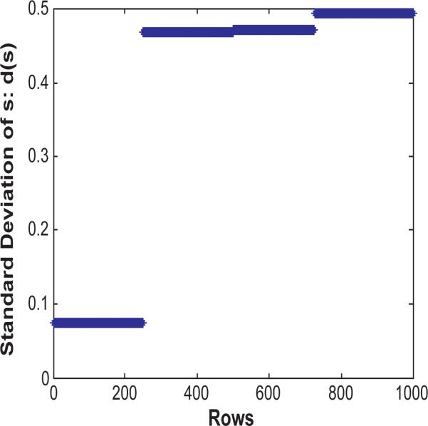
Consider the scenario where an existing row cluster ${\widehat{r}}_j=\{{\mathbf{r}}_{j_1},\dots ,{\mathbf{r}}_{j_a}\}$ is not sampled in M_R, then for each row vector ${\mathbf{r}}_{j_i}\in {\widehat{r}}_j$, all of the m′ row vectors in M_R are almost equally irrelevant to r_ji. Thus if we calculate the label vectors of r_ji according to Equation 15, it is expected that the standard deviation of the elements in s is very low.

Let d(s) denote the standard deviation of the elements in s. An example is shown in Figure 6. The figure plots d(s) for each row in one iteration of the co-clustering. The first 250 rows form a cluster in the data. However, none of them is selected in M_R. As we can see, for those rows, d(s) is much lower than other rows which belong to properly sampled clusters.

Figure 6.

Standard deviation of label vectors

In CRD, we use Chebyshev's Inequality to detect those rows and columns. Consider d(s) of all rows(columns) as a distribution with expected value μ and standard deviation σ, Chebyshev's inequality entails that, for any real number q > 0 we have the conservative bound:

$$Pr(\mid d\left(s\right)-\mu \mid \ge q\sigma )\le \frac{1}{q^2}$$ (18)

We set q = 2 in CRD, i.e., if there are more than $\tau =\frac{1}{q^2}=25\%$ of the rows (columns) having |d(s) − μ| ≥ 2σ, the algorithm will quit the iteration and re-sample the rows (columns).

In general, larger τ induces lower re-sampling frequency and shorter runtime while smaller τ induces higher re-sampling frequency and longer runtime. Since Chebyshev's Inequality holds for any distribution, $\frac{1}{q^2}$ is a rather loose bound. In fact, we found in the experiments that the bound $\tau =\frac{1}{q^2}=25\%$ is too loose and does not induce re-sampling sufficiently. Therefore we test various values of τ to obtain the optimal frequency of re-sampling. Based on our experiments on both real and synthetic data, instead of 25%, τ = 12.5% has the best tradeoff between runtime and cluster purity (as defined in Section 6).

In Steps (5,8) of Figure 5, we calculate d(s) for each row(column). If the percentage of rows (columns) having |d(s) − μ| ≥ 2σ is larger than τ, the re-sampling works in the following way.

• All the rows(columns) that are already in M_R (M_C) will be kept.

• If the number of rows(columns) having d(s) ≤ μ − 2σ is t, then $\frac{t{m}^{\prime }}{m}$ rows ($\frac{t{n}^{\prime }}{n}$ columns) will be randomly re-sampled only from this set of rows (columns).

• When adding new rows/columns into M_R and M_C, they must not violate Constraints 1 ~ 3 in Definitions 3.1 and 3.2.

Note that in Step (5) of Figure 5, only rows are re-sampled, and in Step (8), only columns are re-sampled.

The re-sampling only involves the calculation of a new B_U which is very fast. B_C and B_R only need to be expanded to include the new columns and rows.

After the re-sampling, the iteration will start over again. In Step (1), those rows (columns) that are already in M_R (M_C) will retain their cluster labels obtained before the re-sampling. All the new rows (columns) will start with the same new cluster label, e.g, β_R(r) = k + 1 (θ_R(c) = l + 1).

In general, CRD has runtime complexity O(t(km′n + ln′m + m′m + n′n)) plus the time used in matrix decomposition, O((m + n)m′n′). For large dataset, it's easy to get m′ << m and n′ << n, and CRD can be orders of magnitude faster than the previous co-clustering algorithms that have runtime complexity at least O(t(k + l)mn).

6. EXPERIMENTS

In this section, we present results on both synthetic data and real data. In order to demonstrate the effectiveness and efficiency of our CRD algorithms, all the datasets have large number of rows and columns. Several other co-clustering algorithms were also implemented for comparison.

Datasets

We use two real datasets and one synthetic dataset in our experiments.

• Multiple Features Dataset²: This dataset consists of features of handwritten numerals (‘0’–‘9’) extracted from a collection of Dutch utility maps. It contains 2000 numerals (rows) and 240 features. There are 10 classes in the dataset (from 0 to 9) and each of them has 200 numerals.

• 20 Newsgroup Dataset³: The package consists of 20000 documents from 20 major newsgroups. Each document is labelled by the major newsgroup in which it is involved. We preprocess the 20 Newsgroup dataset to build the corresponding two dimensional contingency table. Each document is represented by a row in the table and 2000 distinct words are selected to form 2000 columns. Words are selected using the same method as that in [17].

• Synthetic dataset: We generated a set of synthetic data with different sizes and noise levels. Each synthetic data is an m × m square matrix consisting of 0 and 1. Co-clusters are embedded by setting different blocks in the matrix to be 1. And we use parameter e to control the noise level, i.e., the value of each element can be randomly flipped with probability e.

Algorithms

We implemented two versions of our CRD framework using different iterative single side clustering approaches.

• CRD-ITC: CRD using information-theoretic co-clustering [5].

• CRD-kmeans: CRD using Euclidian distance (k-means) co-clustering [1].

Unless otherwise noted, we set q = 2 and use bound τ = 12.5% for re-sampling in the CRD algorithms.

In order to show the efficiency of our CRD framework, we also implemented three recent co-clustering algorithms.

• ITC: the original information-theoretic co-clustering algorithm without matrix decomposition[5].

• Kmeans: the original Euclidian distance co-clustering algorithm without matrix decomposition[1].

• ONMF: the orthogonal nonnegative matrix tri-factorization co-clustering algorithm proposed in [8].

Performance Measurement

In the experiments, we compare the runtime and purity of co-clustering solution of the algorithms.

The purity measurement was used in [8]. The purity of a clustering solution is calculated as the weighted sum of the purity of each cluster and is given by,

$$purity=\sum _{i=1}^k\frac{m_i}{m}{P}_i,P_i=\frac{1}{m_i}ma{x}_{j\in [1,k]}\left(m_i^j\right)$$

where m is the total number of rows(columns), m_i is the size of cluster i and $m_i^j$ is the number of rows(columns) in cluster i that has (real) class label j. The larger the value of purity, the better the clustering is.

In the real datasets, since we only know the true class labels of the rows, the purity is only calculated and compared on row clusters. While in the synthetic data, we compare the purity of both row and column clusters found by co-clustering.

All algorithms were implemented in MATLAB. All experiments were conducted on a PC with CPU P4 3GHz, 1G RAM and 80G HDD.

6.1 Synthetic Data

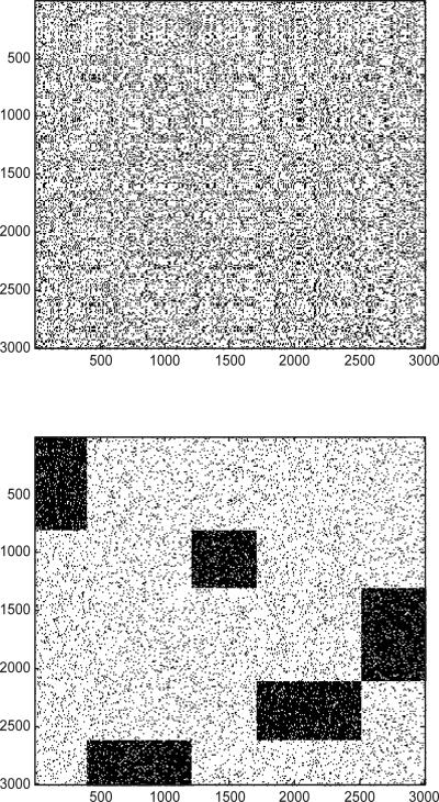
In this section, we compare the performance of the algorithms on a set of synthetic data. For each synthetic dataset of size m × m, we embed 5 row/column clusters into the matrix. An example dataset of size 3000 × 3000 is shown in Figure 7. The figure at the top plots the original data matrix: the dark point represents the ’1’ elements in the matrix. And the figure at the bottom shows the co-cluster structure after the orders of the columns/rows are rearranged.

Figure 7.

Example of a synthetic data matrix of size 3000×3000

We vary the following parameters separately in the experiments:

• m: size of synthetic data matrix (for both row and column). Default value, 5000.

• e: noise level of synthetic data. Default value, 0.1.

• m′: number of selected rows (columns) in low rank row/column decomposition when using CRD. Default value, 20.

When varying one of the parameters, the rest use their default values.

Varying m

By varying m, the number of rows and columns in the data matrix are changed simultaneously, e.g., when m is doubled, the data matrix will have size 2m × 2m. We vary m from 3000 to 11000. The runtime and row/column cluster purity of the algorithms are plotted in Figures 8 and 9.

Figure 8.

Runtime performance when varying m

Figure 9.

Purity performance when varying m

As we can see, CRD algorithms are orders of magnitude faster than the other three algorithms. ONMF is the slowest algorithm because it uses more iterations to converge. When m becomes larger than 9000, the entire matrix is too large to be loaded into the MATLAB environment. Therefore, we did not get any results for ITC, Kmeans and ONMF for m ≥ 9000. While for our CRD algorithm, there is no problem for such large matrices, since it only needs to load {M_C, W_C, M_R, W_R} which are much smaller.

The runtime of calculating the low rank row/column decomposition is shown in Figures 8 at the bottom. The decomposition is very efficient. It only takes a small portion of the total runtime of CRD algorithms. When m ≥ 9000, since the data matrix cannot be entirely loaded, our decomposition algorithm have to load the matrix piece by piece when calculating the norm of each column and row. That's the reason for the steep change in runtime when m passes 9000.

The purity of all algorithms decreases when we increase the number of rows/columns in the matrix. One reason is that the increasing number of rows/columns (with noise) brings more local optimums into the data, which makes it more difficult for the algorithms to find the embedded co-clustering structure. The purity of CRD algorithms is comparable to that of the other algorithms as shown in Figure 9. Thus, the dramatic saving in its running time makes CRD the winner among all algorithms.

Varying e

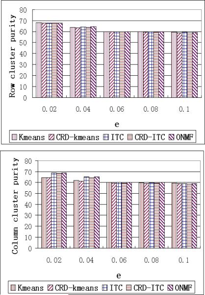
When we increase the value of e, the synthetic data have more noise. The largest row/column cluster embedded in the data covers only 20% of the rows/columns. When e exceeds 0.2, the embedded structure begins to be overwhelmed by noise. Therefore, in this set of experiments, we vary e from 0.02 to 0.1.

The runtime of the algorithms does not change so much with increasing e. So we only report the purity performance in Figure 10.

Figure 10.

Purity performance when varying e

The purity of CRD algorithms is comparable to others but is slightly lower when e becomes larger. One reason is that, the effectiveness (accuracy) of the low rank decomposition is sensitive to the increase in noise. Though we have the re-sampling procedure in CRD, the computation of the updated weight matrices, W_R and W_C, is still affected by the noise.

Varying m′

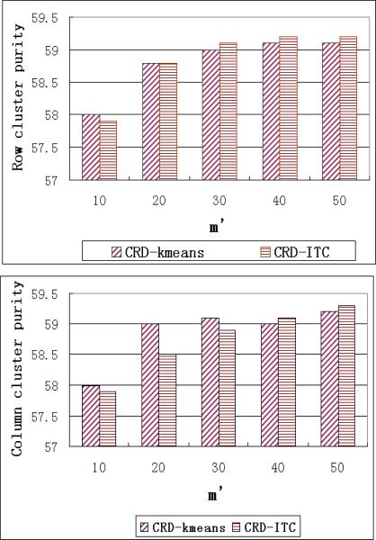
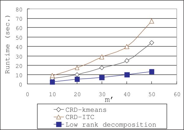
In this set of experiments, we vary the number of selected rows/columns, m′, from 10 to 50. This parameter does not affect the ITC, Kmeans and ONMF algorithms, therefore we only plot the cluster purity and runtime of our CRD algorithms in Figures 11 and 12 respectively.

Figure 11.

Purity performance when varying m′

Figure 12.

Runtime performance when varying m′

As we can see, the CRD algorithms and their pre-processing procedure, the decomposition algorithm, both have runtime increase linearly with respect to m′. Increasing the number of selected rows/columns can also improve the purity of the co-clustering solutions. However, when there are enough rows/columns in M_C and M_R, adding more rows/columns can only affect the purity slightly. As shown in Figure 11, when there are more than 30 rows/columns, the improvement of purity becomes very small.

Efficiency of Re-sampling

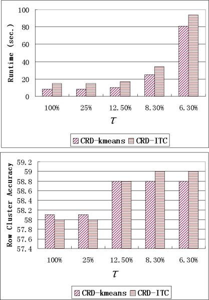
As we discussed in Section 5.2, the random sampling of matrix decomposition does not guarantee to sufficiently sample all cluster structures and re-sampling is used in CRD to make up for the missing clusters in random sampling. We use Equation 18 to detect those rows/columns that are not properly sampled. For all the previous experiments we set q = 2 and use bound τ = 12.5%, i.e., if there are more than 12.5% of the rows (columns) having |d(s) − μ| ≥ 2σ, the CRD algorithm will re-sample the rows (columns).

In order to show the effects of τ on re-sampling frequency and clustering performance, we vary τ from 100% to 6.3% in this set of experiments. Note that when the τ is equal to 100%, the CRD algorithm does not re-sample rows/colums in any case. The results on the 5000 × 5000 synthetic data are shown in Figure 13. Column cluster purity is omitted because it is similar to the row cluster purity.

Figure 13.

Runtime and Row cluster purity performance with different re-sampling bound τ

Considering runtime and clustering performance together, τ = 12.5% has the best performance. When τ = 25%, there is almost no re-sampling in CRD. When τ is set to 6.3%, the algorithm consumes much longer time but has no significant improvement in clustering performance. There are two reasons for the longer runtime when bound= 6.3%

• More frequent matrix decomposition computation.

• Larger size of {W_R, M_R, W_C, M_C}.

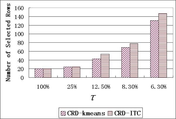
The numbers of selected rows for these bounds are shown in Figure 14. As we can see, when τ = 25%, only a few rows are re-sampled. And when τ = 6.3%, there are too many rows selected in the M_R matrix.

Figure 14.

Number of selected rows with different re-sampling bound τ

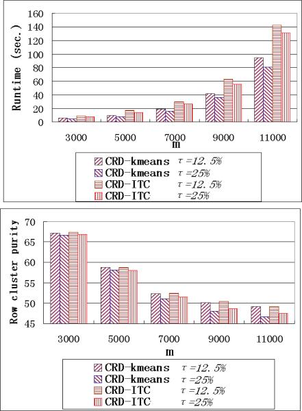
We also use τ = 25% and τ = 12.5% on datasets of different sizes and compare the performance. The results are shown in Figure 15. As expected, the runtime of the CRD algorithms with τ = 25% is always slightly faster. However, its purity of row clustering is lower than that of the CRD algorithms with τ = 12.5% especially when there are a large number of rows and columns in the data matrix, e.g., m ≥ 9000. In those cases, the initial low rank decomposition may have a larger risk to miss a cluster or sample insufficiently in a cluster with a mixed number of selected rows (columns), and the re-sampling steps becomes more important.

Figure 15.

Runtime and Row cluster purity performance of τ = 25% and τ = 12.5% on data of different sizes

6.2 Multiple Feature Dataset

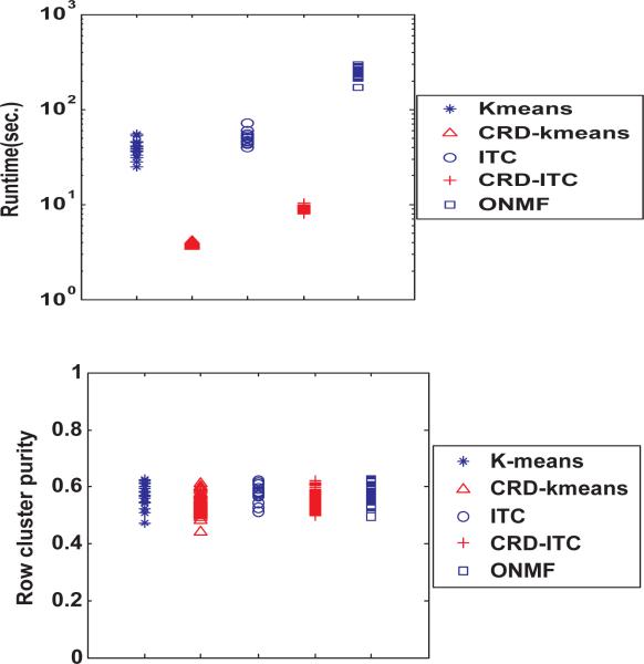
The multiple feature dataset contains 2000 rows and 240 columns. And the 2000 rows are equally divided into 10 classes. We run each algorithm 40 times on the dataset, and plot the distribution of their runtime and row cluster purity in Figure 16. Since the columns do not have class label, the column cluster purity cannot be calculated here.

Figure 16.

Runtime and Row cluster purity performance on Multiple Feature Dataset

Each point in Figure 16 represents the runtime or the purity of a single run of one of the algorithms. As we can see, our CRD algorithms are about 10 times faster than ITC and Kmeans and more than 20 times faster than ONMF. The performance advantage of the CRD algorithms is not as much as the one on the synthetic data because the multiple feature dataset has much less columns than rows, and thus most of the speedup comes from the row-side sampling only.

And if we compare the distributions of cluster purity in Figure 16, we can find that CRD algorithms performs as good as the other three algorithms.

6.3 20 Newsgroup Dataset

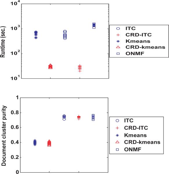
In this section, we use the 20 newsgroup dataset to compare the performance. The entire data matrix is too large to be loaded into MATLAB environment, therefore, we use a subset of the dataset which contains 5000 documents from 5 newsgroups. And 2000 words are selected as features using the same method as in [17]. We run each algorithms 10 times on the dataset and plot the distribution of runtime and row (document) cluster purity in Figure 17. Words do not have class label so that the purity of word clusters cannot be calculated.

Figure 17.

Runtime and Document cluster purity performance on 20 Newsgroups Dataset

CRD algorithms are still orders of magnitude faster than the other three algorithms. The Euclidian distance based algorithm, Kmeans and CRD-kmeans, cannot cluster the documents correctly and have much lower purity than others. ITC, CRD-ITC and ONMF has similar performance on document cluster purity.

The low rank decomposition on these two real datasets is fast and the runtime can be neglected.

Based on the experiment results we presented in this section, we can see that our CRD framework can be used to design co-clustering algorithms which are much faster and can achieve comparable co-clustering accuracy.

7. CONCLUSIONS

In this paper, we proposed a general framework for fast co-clustering on large data, CRD. CRD has two components. It first decomposes the data matrix into low rank row/column approximation matrices. Then co-clustering algorithms using iterative single-side clustering are used to cluster the approximation matrices. Several constraints are added in the matrix decomposition in order to ensure the performance of co-clustering. Because of the small size of the approximation matrices, CRD has runtime complexity O(t(km′n + ln′m + m′m + n′n)) which is orders of magnitude faster than O(t(k + l)mn), which is the runtime complexity of the previous co-clustering algorithms. We conducted experiments extensively on real datasets and synthetic datasets. The results show that our framework is both efficient and effective.

8. REPEATABILITY ASSESSMENT RESULT

Figure 8 (when m = 3000 and 5000), Figure 16 and Figure 17(top) have been verified by the SIGMOD repeatability committee.