DETERMINING RNA THREE-DIMENSIONAL STRUCTURES USING LOW-RESOLUTION DATA

Abstract

Knowing the 3-D structure of an RNA is fundamental to understand its biological function. Nowadays X-ray crystallography and NMR spectroscopy are systematically applied to newly discovered RNAs. However, the application of these high-resolution techniques is not always possible, and thus scientists must turn to lower resolution alternatives. Here, we introduce a pipeline to systematically generate atomic resolution 3-D structures that are consistent with low-resolution data sets. We compare and evaluate the discriminative power of a number of low-resolution experimental techniques to reproduce the structure of the Escherichia coli tRNA^VAL and P4-P6 domain of the Tetrahymena thermophila group I intron. We test single and combinations of the most accessible low-resolution techniques, i.e. hydroxyl radical footprinting (OH), methidiumpropyl-EDTA (MPE), multiplexed hydroxyl radical cleavage (MOHCA), and small-angle X-ray scattering (SAXS). We show that OH-derived constraints are accurate to discriminate structures at the atomic level, whereas EDTA-based constraints apply to global shape determination. We provide a guide for choosing which experimental techniques or combination of thereof is best in which context. The pipeline represents an important step towards high-throughput low-resolution RNA structure determination.

Ribonucleic acid (RNA) is one of the central molecules of cellular information transfer [1,2]. Characterizing how RNA participates in chemical reactions increases our comprehension of how cells function. Structure is one of our best hints about RNA function, and so high-resolution methods such as X-ray crystallography and nuclear magnetic resonance (NMR) spectroscopy are routinely applied to determine RNA three-dimensional (3-D) structures. However, these methods can neither be applied to all RNAs nor in all cellular conditions.

Alternatively, RNA 3-D structures can be predicted computationally or modelled interactively [3-7]. However, one of the problems with computational structure prediction is that they generate sets of geometrically different but energetically similar structures, making difficult the selection of native structures. The problem may be partially related to the fact that RNA structures are dynamics, and thus have the potential to accommodate various reactions under different conditions [8]. For instance, riboswitch, ribozyme, and microRNA structures are subject to conformational induction in presence of their respective cofactors [9].

To help sort through many plausible structures, much effort is being invested in using low-resolution experimental techniques and data. These techniques include variants of hydroxyl radicals (OH) footprinting [10], for instance the ethylenediaminetetraacetic acid (EDTA) variants uridine-EDTA [11] and methidiumpropyl-EDTA (MPE) [12], and the multiplexed hydroxyl radical cleavage analysis (MOHCA) [13].

Cleavage of the RNA backbone by OH provides a way to distinguish the inside and outside of a folded RNA molecule [14]. As the RNA folds in its native state, sections of the backbone may become protected from the solvent. The backbone atoms that are buried inside the RNA are less prone to OH attacks and cleavage. Therefore, OH footprints give the accessibilities of nucleotides’ backbone atoms; the greater the cleavage activity is the more accessible the nucleotide is. The OH footprints are gel-based and amenable to robust and automated analysis [15].

EDTA variants are also gel-based [11,12]. The idea behind these techniques is to insert an Fe(II)-EDTA moiety acting as a probe at a specific position. Then, the backbone cleavage pattern defines the accessibility of a nucleotide and its approximate distance to the probe. RNA selective 2′-hydroxyl acylation analysed by primer extension (SHAPE) [16,17] is a technique that is getting popularity in the RNA community. It is used to measure the dynamics of nucleotides in an RNA structure, and thus is extremely powerful to determine secondary structure [3,18,19], i.e. the stable nucleotides are considered involved in stacked Watson-Crick base pairs. For instance, using SHAPE data the Miller group has modelled the cap-binding translation initiation factor eIF4E bound to a pseudo-knotted element [20], and the Perreault’s group modelled putative folding intermediates of the HDV ribozyme [21]. However, it is not clear how SHAPE data can be interpreted and used in the context of 3-D structure. Nevertheless, EDTA combined with SHAPE data and a force-field based on a united nucleotide representation [5] were used to reproduce a tRNA with an accuracy of less than 4 Å of root-mean-square deviations (RMSD) between the Phosphate atoms of the model and that of its corresponding experimental structure [12].

MOHCA is another gel-based probing technique that uses EDTA [13]. First, an EDTA probe cleavage agent is randomly inserted in the structure. Then, the positions of radical hydroxyl cleavages are read in a two-dimensional gel against the positions of the probe, producing a set of pairwise distance constraints. The distance between a cleavage site and the probe is proportional to the intensity of the cleavage. The analysis of MOHCA data has recently been automated [22]. More recently, the application of small-angle X-ray scattering (SAXS) technique [23,24] has been applied to RNAs. It is currently considered a promising technique that may be used to accelerate the systematic resolution of RNA structures. A nice example of its application was done by the Doniach’s group who used SAXS data to determine the bound and unbound states of the thiamine pyrophosphate riboswitch [25]. To get SAXS data, one bombards the RNA in solution with X-rays, and then measures how the scattering varies on average over all orientations of the RNA and according to small angular changes of the X-ray beam [26].

SAXS data can be used in two different ways. The first is by comparing directly a theoretical scattering curve with that obtained experimentally. The most widely used computer programs that implement this approach are CRYSOL [27] and DAMMIN [28]. CRYSOL generates a theoretical scattering curve from an actual 3D model, whereas DAMMIN does it from a model made of beads of a fixed size that approximates the atomic density of an unknown 3D structure. One can generate a 3-D model that fits the bead model, for instance by using rigid body molecular docking. The model’s theoretical curve is then compared to the experimental one, and the difference between them is measured. Little or no difference between the two curves indicates that the model satisfies the SAXS data.

The second is by applying a Fourier transform on the scattering curve to obtain a pair-density distribution function (PDDF), which represents the pairwise distance distribution between the electrons of the molecule. The computer program GNOM has been developed to compute such a PDDF [29].

Our goal to develop a pipeline for determining RNA 3-D structures using low-resolution data prompted us to consider the structural data generated by the above techniques. Such data translate into geometrical constraints, and thus can be directly used to guide structure generation algorithms towards satisfying solutions. However, tuning an algorithm to use specific types of structural data is time consuming. Since the discriminating power of these data has not been tested in the context of high-throughput 3-D structure determination, we decided as a first step to compare their discriminative power to identify experimentally resolved structures from existing sets of theoretically generated atomic structures (Fig. 1).

Figure 1. Steps for determining RNA 3-D structures using low-resolution data.

a) Sequence input. The input of the pipeline is an RNA sequence. b) Structure prediction. 3-D structure sets are produced using an RNA structure generator capable of simultaneously sampling the global shape and producing atomic-resolution models of the RNA input sequence. The 3-D structure generator can benefit from secondary structure prediction, which is an optional step. If used, however, then more than one secondary structure can be selected and used to produce 3-D structures. The 3-D structure sets (Decoys) represent intermediate results, but they can also be stored permanently for future use. c) Experimental data collection and filtering. The experiments may include, but are not restricted to: hydroxyl radical footprinting (OH); methidiumpropyl-EDTA (MPE); multiplexed hydroxyl radical cleavage analysis (MOHCA); and, small-angle X-ray scattering (SAXS). OH experiments show on a gel the nucleotides that are protected from cleavage upon folding. The OH data can be exploited by assessing the loss of solvent accessibility of these protected nucleotides (red spheres). MPE experiments show the cleavage intensity when the MPE agent is attached at a given position, here at nucleotide 67 in the tRNA (green sphere). MPE data can be used to estimate the distance to the MPE agent of the cleaved sites (red spheres). The distances are proportional to the cleavage intensity, which can be visualized using a histogram. MOHCA experiments result in distances between marked positions (red sphere) and the MOHCA agent (green sphere). The measured intensities are proportional to the distance between a marked position and the agent. SAXS experiments show the intensity of the scattering measured at different angles. SAXS data are convoluted and requires Fourier transforms to be converted into distance probabilities. Here, a theoretical SAXS scattering curve was generated from a tRNA 3-D model (grey spheres) and water atoms surrounding the tRNA (yellow spheres). The theoretical curve is then compared with the experimental one for congruence at all scattering angles. d) 3-D structure output. Filtering 3-D structure sets using single or combinations of experimental data results in subsets of 3-D structures that satisfy the low-resolution data. These structures can be analysed further, and submitted to energy minimization or molecular dynamics protocols for refinement.

The comparison was done using two well-studied RNAs: the Escherichia coli valine tRNA (tRNA), which has been solved in solution (PDB code 2K4C [30]), and the group I intron of the Tetrahymena thermophila P4-P6 domain (P4-P6), which structure has been determined by X-ray crystallography (PDB code 1GID [31]). These structures have also been used as benchmarks for RNA secondary and 3-D structure prediction methods [6,12,13,32], and structure probing data for these two RNAs are available.

To challenge the above RNA structure probing techniques thoroughly, we needed an RNA structure generator capable of sampling the accessible shapes and producing atomic resolution models of the tRNA and P4-P6 domain. The atomic precision is needed to assess properly the reproduction of the base pairing and stacking conformations, as well as the proper volume, electron density, and quality of the backbone path.

We chose the most recent version of the MC-Sym computer program [3,33,34], which combines the desired attributes. MC-Sym implements a fragment-based construction algorithm [3]. It merges 3-D fragments that correspond to nucleotide cyclic motifs (NCMs) [35]. The 3-D fragments are either directly taken in the Protein DataBank RNA structures if instances of the exact sequence exist, or automatically built otherwise. The automated fragment building procedure guarantees the generality of the approach and that the MC-Fold and MC-Sym pipeline applies to never previously observed sequences.

The first step is thus to describe the RNA in terms of NCMs, i.e. to identify the single-stranded fragments closed by a single base pair (i.e. hairpin loops) and double-stranded fragments that are flanked by two base pairs (i.e. tandem of base pairs, and bulge and interior loops). For instance, the MC-Fold and MC-Sym pipeline automates this process [3], but an input script can always been edited or defined manually. Here, the MC-Sym input scripts were directly derived from pre-established and known secondary structures (see Materials and Methods). In cases where the secondary structure of a new RNA has not previously been determined, the first step would then to predict it using MC-Fold. Note that any secondary structure prediction method would do here. The difference between thermodynamics approaches and MC-Fold is that the latter uses a scoring function based on the statistics of occurrences of the NCMs in known 3-D structures. Base pairing and stacking, as well as backbone effects are inherent to the NCMs. MC-Fold uses a Markov chain of NCMs of order one, which allows to embed indistinctly all contextual energetic contributions. As a result, MC-Fold produces secondary structures that are enriched by non-canonical base pairs, and thus provide key structural information for building 3-D structures. There is an MC-Fold and MC-Sym pipeline Web service available at www.major.iric.ca. Alternatively, both programs can be downloaded and run on desktop computers. There is also an application that converts an RNA secondary structure represented by a dot-bracket string into an MC-Sym input script (see Materials and Methods).

Note that many non atomic-precision modelling systems could also be used. They generate RNA models to which all atoms can be added in a later step. NAST [6,36], iFoldRNA [5,37], RNA2D3D [7], and the recent approach proposed by Cao and Chen [38] are such examples. Recently, the Levitt’s group has also developed an in silico approach to generate sets of RNA 3-D structures by clustering RNA conformations constrained by secondary structure alone [39]. As it will be shown below, this approach can be very powerful when combined to filtering using low-resolution experimental data.

Results

Conformational sampling

Similarly to the Levitt’s group approach, for each RNA we built two sets of 3-D models. The first set is termed “low”, where we only consider secondary structure and coaxial stacking information (see Fig. 2 and 3, Top). The second set is termed “high”, where we also provide additional long-range tertiary base pairs (see Fig. 2 and 3, Bottom). For the tertiary base pairs, we took advantage of the structural data that have previously been inferred from sequence co-variation analysis [40-42].

Figure 2. tRNA conformational sampling.

(Top) Low set. a) Secondary structure coloured by stems: Acceptor (green); D (cyan); Anticodon (orange); and, T (yellow). All other nucleotides are in magenta. b) Two views of twenty centroids (thin tubes) that are optimally aligned on the solution structure (PDB file 2K4C, thick tube). The colours are the same as in a. c) RMSD (Å) range (all-atoms) of the low set models computed against the tRNA experimental structure (PDB code 2K4C). (Bottom) High set. d) The secondary structure, three base triples (8-14-21, 9-12-23, and 13-22-46), and three long-range base pairs (15-48, 18-55 and 19-56) shown using dashed lines. e) Two views of twenty centroids (thin tubes) that are optimally aligned on the solution structure (PDB file 2K4C, thick tube). The colours are the same as in d. f) RMSD (Å) range (all-atoms) of the high set models computed against the tRNA experimental structure (PDB code 2K4C).

Figure 3. P4-P6 conformational sampling.

(Top) Low set. a) Secondary structure coloured by stems: P4-P5 (green); P5a (orange); P5b (cyan); and, P6 (yellow). The other nucleotides are in magenta. The nucleotides that were not sampled are uncoloured. b) Two views of twenty centroids (thin tubes) that are optimally aligned on the crystal structure (PDB file 1GID, thick tube). The colours are the same as in a. c) RMSD (Å) range (all-atoms) of the low set models computed against the P4-P6 crystal structure (PDB code 1GID). (Bottom) High set. The A-minor long-range base pair (A153-G250) is added in the constraints (circled nucleotides and dashed line). d) Two views of twenty centroids (thin tubes) that are optimally aligned on the crystal structure (PDB file 1GID, thick tube). The colours are the same as in a. e) RMSD (Å) range (all-atoms) of the high set models computed against the P4-P6 crystal structure (PDB code 1GID).

Figures 2 and 3 show the conformational samplings and distributions of RMSD over all-atoms between the models and their corresponding experimental structures. For the tRNA, the RMSD range from about 6.1 up to 25.1 Å (Fig. 2c) and 3.6 up to 12.4 (Fig. 2f) for the tRNA low and tRNA high sets respectively. For the P4-P6 domain, which contains twice the number of nucleotides vs. the tRNA, that is 158 vs. 76, the RMSD range from 13.1 to 49.4 Å (Fig. 3c) and 6.9 to 14.2 Å (Fig. 3e) for the low and high sets respectively. Worth noting is that the inclusion of very few long-range 3-D contacts (see Materials and Methods) significantly affect the RMSD distributions of the generated models. For instance, the RMSD peaks go from 17 down to 5 Å and from 43 down to 9 Å for the tRNA and P4-P6 respectively.

Discriminative power of low-resolution experimental data

To assess the relative discriminative power of the considered experimental techniques, we compute the correlation between their corresponding experimental data fitness and the RMSD between the 3-D structures (Decoys) and the corresponding native structure (see Fig. S1 and S2). A different fitness measure is defined for each experimental data type (see Materials and Methods).

A visual inspection clearly shows that the best correlation is from using MOHCA on the P4-P6 low set (r² = 0.995; Fig. S2b). The next-best is SAXS, again on the P4-P6 low set (r² = 0.347 in the RMSD region below 25 Å; Fig. S2c), as well as on the tRNA low set (r² = 0.234; in the RMSD region below 15 Å; Fig. S1c). The r² is below 0.2 for all other data and model sets, indicating that for any given fitness value many different models would qualify and for any given RMSD to the native structure we observe a wide range of fitness values.

The correlation of MPE on the tRNA low set is r² = 0.158 (Fig. S1b). The problem of selecting one or a few models that represent the native fold is thus complicated in this case. One cannot simply pick the model that best fit the experimental data because the range in RMSD is quite large. Another bad example is the large RMSD range of the OH fit above the 0.5 line shown in Figure S1a. We reinterpreted the MPE data (see Materials and Methods), but we can that neither the MPE^* nor MPE^** can identify a model that is native-like.

Therefore, we devised a model selection procedure (see Materials and Methods) that yields a handful of similar models that collectively best fit the experimental data. The results of applying the model selection procedure on all sets are presented in Tables 1 (tRNA) and 2 (P4-P6). For each individual and combination of experimental techniques, the mean RMSD and Global Distance Test (GDT-TS [43,44]) are shown. These measures show how close the selected models are compared to the native structure. The model selection procedure is robust, as indicated by the small RMSD standard deviations (around 1.0 Å on low and 0.5 Å on the high sets) among the selection cycles (see the values in parentheses in the RMSD column in Tab. 1 and 2).

Table 1. Performance of experimental data for the tRNA model sets.

The first three columns are the experimental data sets: OH (hydroxyl radical footprinting); MPE (methidiumpropyl-EDTA); and, SAXS (small-angle X-ray scattering). The dots indicate the experimental data considered in the model selection procedure. <RMSD> is the average RMSD in Å for 100 selection procedures. <GDT-TS> is the average GDT-TS for 100 selection procedures. N indicates the total number of structures selected. Q is the percentage of structures in the set that have lower RMSD than <RMSD>. Values in parenthesis are the standard deviations. Details of the model selection procedure and GDT-TS computation are given in Materials and Methods

Experiment			Resolution
OH	MPE	SAXS	<RMSD>	<GDT-TS>	N	Q
tRNA low [6.1, 25.1] Å
•			15.92 (0.64)	0.07 (0.01)	2406	51.5
	•		10.97 (0.57)	0.10 (0.02)	3277	11.6
		•	9.11 (1.10)	0.20 (0.05)	2974	3.2
•	•		10.09 (0.98)	0.14 (0.03)	3997	7.0
•		•	9.16 (1.06)	0.18 (0.03)	4241	3.3
	•	•	11.32 (0.65)	0.10 (0.01)	3276	14.3
•	•	•	9.46 (1.06)	0.17 (0.04)	4798	4.4
tRNA high [3.6, 12.4] Å
•			5.46 (0.81)	0.38 (0.81)	2535	36.9
	•		5.71 (0.20)	0.35 (0.20)	2566	47.0
		•	6.56 (0.19)	0.30 (0.02)	1649	74.4
•	•		5.55 (0.20)	0.38 (0.02)	2043	40.6
•		•	6.26 (0.49)	0.33 (0.03)	2890	65.8
	•	•	7.51 (0.52)	0.25 (0.02)	1995	90.8
•	•	•	6.34 (0.56)	0.31 (0.03)	2760	68.8

Table 2. Performance of experimental data for the P4-P6 model sets.

The first three columns are the experimental data sets: OH (hydroxyl radical footprinting); MOHCA (multiplexed hydroxyl radical cleavage analysis); and, SAXS (small-angle X-ray scattering). The dots indicate the experimental data considered in the model selection procedure. <RMSD> is the average RMSD in Å for 100 selection procedures. <GDT-TS> is the average GDT-TS for 100 selection procedures. N indicates the total number of structures selected. Q is the percentage of structures in the set that have lower RMSD than <RMSD>. Values in parenthesis are the standard deviations. Details of the model selection procedure and GDT-TS computation are given in Materials and Methods

Experiment			Resolution
OH	MOHCA	SAXS	<RMSD>	<GDT-TS>	N	Q
P4-P6 low [13.1, 49.4] Å
•			43.78 (1.79)	0.01 (0.00)	2770	84.0
	•		16.57 (0.50)	0.06 (0.01)	2558	0.4
		•	17.46 (1.17)	0.05 (0.01)	3029	0.7
•	•		19.76 (1.59)	0.04 (0.01)	3234	1.9
•		•	16.72 (1.18)	0.06 (0.01)	2382	0.4
	•	•	17.35 (1.19)	0.06 (0.01)	2695	0.6
•	•	•	17.57 (1.27)	0.05 (0.01)	2799	0.7
P4-P6 high [6.9, 14.2] Å
•			9.47 (0.09)	0.33 (0.00)	7556	52.5
	•		8.76 (0.21)	0.27 (0.01)	2939	21.8
		•	10.34 (0.34)	0.22 (0.01)	887	81.2
•	•		8.30 (0.16)	0.27 (0.02)	1735	11.5
•		•	7.48 (0.05)	0.35 (0.00)	6128	2.0
	•	•	8.42 (0.09)	0.31 (0.00)	6765	14.4
•	•	•	7.48 (0.07)	0.35 (0.00)	6834	2.0

An interesting measure is the Quantile-value (Q), which is the percentage of models in a set that have lower RMSD than that of a given one. For instance, a model with a Q of 0.5% indicates that less than 0.5% of the models in the set have better RMSD than it. The highest possible Q is 100.0% for the model that has the highest RMSD, since all other models have lower RMSD than it. Similarly, the model with the best RMSD has a Q of 0.0%. Low Q values indicate that the selection procedure is not a random one. If it were random, then the Q values would be near the median or the mean RMSD in each case (see Fig. 2 and 3).

On the low sets, SAXS seems to be the best technique for both RNAs (Q = 3.2% and 0.7% for the tRNA and P4-P6 respectively). MOHCA performs well, but only on the P4-P6 low set (Q = 0.4%). MPE on the tRNA low set is less selective, Q = 11.6%, than SAXS. Note that in practice, any valuable experimental probing technique is one that can select a manageable number of 3-D models. For instance, a Q value around or below 3.5% for sets of 100,000 models selects less than 3,500 3-D models that can easily be clustered and analysed.

Importantly, OH footprinting is of no help to discriminate models that are far from the native structure. However, as the models get closer to the native fold, OH footprinting becomes increasingly discriminative. See for instance in the case of the P4-P6 domain, the model selection procedure for the high set identifies models of 2.0% and 11.5% Q values, respectively for OH+SAXS and OH+MOHCA (Tab. 2). In the case of the tRNA high set, when only OH data are considered we get Q = 36.9%, or Q = 40.6% when OH+MPE data are considered (Tab. 1). Worth noting is that OH data have been exploited in conjunction with MOHCA for the reproduction of the native fold of the P4-P6 domain [13].

Discussion

Following the recent enthusiasm for RNA structure and development of new RNA 3-D modelling systems, one of the goals of this work was to assess the current resolution and predictive power of a current system when used in combination with various types of low-resolution experimental data. We chose a representative RNA 3-D structure generation algorithm, MC-Sym, and addressed the question whether we could build a high-throughput low-resolution RNA 3-D structure determination system. We were not as much interested in finalizing such a system now, but rather curious about the accuracy one could achieve with such a system at this time. We thus idealized the modelling conditions and determined how different types of experimental data could be used to filter the best possible RNA 3-D structure prediction sets.

Lessons for the experimentalists

The observation of quite high Q values (> 35%) for the high tRNA set (Tab. 1) indicates that either: i) the models in the high set are too accurate for the resolution of the experimental data tested here; or, ii) the tRNA is too small or compact to make a notable difference upon substantial conformational changes, i.e. the lengths of the probes are comparable to its radius of gyration. Given that during tRNA folding many conformations can be explored [45], it would be interesting to compare buffer solutions between the MPE-based probing and that of SAXS, for instance, or to revisit how the EDTA-based probing data should be interpreted. That being said, the radius of gyration of the tRNA has been measured to be about 23.5 Å [46], which is within the range of the tether probe. Besides, MOHCA has the drawback of using a bulky and potentially perturbing agent that can modify the RNA structure under study. SAXS+OH data have an excellent discriminative power for the “low” data sets, and has the advantage of probing an unmodified RNA.

The level of structural information used to define the high tRNA set is unusual. To reach the accuracy of 4 Å RMSD with the native structure (high set), all base pairs (including the non-canonical) were needed. We get an accuracy of 7 Å RMSD if we use the secondary structure alone (low set). Thus, determining base interactions beyond secondary structure would be an important asset, either theoretically from sequence data, or experimentally.

MC-Sym is a representative of the best RNA 3-D structure generation algorithms available right now [32,47,48]. This was the first time that low-resolution data were challenged against this type of atomic precision 3-D modelling results on relatively large RNAs. There are generated structures that are closer to the native structures than it is possible to identify with an unbiased selection procedure driven by representative low-resolution experimental data (Tab. 1 and 2). It would be interesting to challenge other experimental techniques, such as SHAPE for instance, and see if they could justify the precision of the structure generator. Unfortunately, we did not look at SHAPE data here because we are currently calibrating MC-Sym for them. By using SHAPE data we would benefit from new types of structural information provided by the: i) 2′OH accessibilities (similar to OH); ii) backbone cleavage; and, iii) nucleotide dynamics. We are looking forward to evaluate the discriminative power of SHAPE data, and to place it in context of recently generated RNA dynamics results [49-51].

Lessons for the theoreticians

The information used to generate the low and high 3-D structure sets were idealized, and we assumed that for both chosen RNAs there exists a single and almost static native structure. The tRNA and P4-P6 domain are exceptionally highly structured RNAs, which served well the purpose of comparing the chosen low-resolution experimental techniques. Note that in many cases, however, there is no such single “correct” structure and high RMSD among the output structures may very well reflect the structural ensemble. It is thus a challenge to detect if high RMSD among the output structures correspond to structural diversity or imprecise structural data. Long-range interactions were extremely useful for the generation of the high structure sets. Long-range interactions provide strong constraints that reduce the conformational search space. However, this is not necessarily the case for all types of experimental data. For instance, it was found that the addition of OH data to that of MOHCA selects worst models than MOHCA data alone, most likely due to “kinetic traps”. The two RNA structure generators that were used in these experiments were FARNA [4] and NAST [6], which are guided by an energy-based function, and hence subject to local minima traps. In comparison, the MC-Sym search algorithm is based on a discrete constraint satisfaction resolution technique that is both sound and complete: i.e. it samples fully an RNA’s conformational space and it builds structures that fully satisfy all input constraints. Here using MC-Sym, we found that incorporating the OH data to that of MPE, MOHCA, and SAXS rather helped the identification of better 3-D models. OH data are thus useful in the context of filtering a set of generated 3-D structures rather than guiding the generation algorithm itself.

The question of secondary structure prediction accuracy is an important one for developing a high-throughput pipeline. The accuracy and prediction of the non-canonical base pairs is needed to build accurate 3-D structures (high sets), and thus a secondary structure prediction method such as MC-Fold is preferred over classical ones. However, including all base pair energetic contributions and considering contextual structural information to increase prediction accuracy comes with higher computational costs resulting in difficulties to address RNA sequences of more than 100 nucleotides (at this time).

MC-Fold and all other secondary structure prediction methods predict a minimum free energy structure and a set of suboptimal structures. As a matter of fact, the minimum free energy structure is often incorrect. Therefore, in the absence of an experimentally validated secondary structure, it is recommended to generate 3-D structure decoys from the minimum free energy secondary structure, but also from a variety of suboptimal ones. The constraint filtering would identify the right secondary structures since their decoys would contain consistent 3-D structures. This approach was applied at a much smaller scale in the case of modelling the pre-catalytic 3-D structure of a lead-activated ribozyme: a series of structural hypotheses were challenged upon chemical modification and catalytic data [47].

There may be ways to improve the computation of fitness. For instance, computing the fitness to OH data is not efficient because it requires the accessible surface area (ASA). However, computing the fitness to MPE data is efficient since it provides distance constraints that can be used either in the model generation process, or as a post-processing step. Computing the fitness of MOHCA data is efficient since it also provides distance constraints. Evaluating the fitness to SAXS data is not efficient since it requires complex numerical computations and must consider the first hydration shells of the footmark on the scattering data, particularly in the case of RNAs.

Availability of the pipeline

The pipeline we introduced here has been made available on-line (www.major.iric.ca) to anyone who is eager to generate sets of RNA 3-D structures and challenge them using experimental data, those that were utilised here and others as well. The pipeline and particularly the model selection procedure identify the models that summarise and represent best any experimental data collection. We must keep in mind that models can explain qualitatively (if not quantitatively) biological function. After all, one of the goals of modelling is to suggest keener experiments that will improve the models and bring more information about function. The pipeline introduced here serves this purpose.

Materials and Methods

Sets of predicted tRNA 3-D structures (Decoys)

We started with the correct secondary structure with the addition of in-stem non-Watson-Crick base pairs, such as the A14-A21, A26-G44, C32-A38, and U54-A58. The T-loop structure fragment was imported from the PDB file 2K4C since it folds independently and in a well-defined motif [52-55]. We also used the Fuller-Hodgson rule for the anticodon loop [56], i.e. we stacked nucleotides 34 to 38 as the prolongation of the helix. The coaxial stacking between the Acceptor and the T stems, as well as between the Anticodon and the D stems was used so that the four stems define two helices [40,57].

The conformational sampling of the low tRNA set was made in three stages. First, we sampled and generated structures for the two helices: axis 1 formed by the T- and acceptor-stem; and, axis 2 by the D- and anticodon-stem. Second, the two helices were positioned relative to each other by sampling the dinucleotide 8-9 conformation. Finally, we completed the tRNA structure by building the D and variable loops by sampling trinucleotides using single-stranded fragments extracted from the PDB.

The conformational sampling of the tRNA high set was also made in three stages. The first stage is identical to that of the tRNA low set, but we selected the conformations of the D-stem that formed the base triples 8-14-21, 9-12-23, and 13-22-46 [41]. We also appended nucleotides 18 and 19 to form the long-range base pairs with the T-loop nucleotides 55 and 56, respectively [40,41]. Second, we positioned the two helices relative to each other using the dinucleotide 7-8. Finally, we added the 15-48 long-range base pair [40,41], and completed the D and variable loops. Figure 2 shows the information used for modelling the tRNA sets, and gives an idea of the conformational search space explored for each.

Sets of predicted P4-P6 domain 3-D structures (Decoys)

We divided the domain into two components: the P5-P4-P6 coaxial stems (axis 1), and the P5a and P5b coaxial stems (axis 2). We extracted the P5c stem and tetraloop receptor from PDB file 1GID. The tetraloop receptor adopts a specific structure that contains an adenosine platform [58] and a UA_handle [59]. In the first stage, we sampled and generated structures for each stem. For the P4-P6 low set, we then positioned the two components relative to each other by sampling the 122-126 and 196-199 strands using trinucleotide fragments extracted from the PDB. Hence, given no other long-range distance constraints, MC-Sym generated P4-P6 domain structures in the familiar U-shape, but also in the L- and flat shapes. For the P4-P6 high set, we added the long-range base pair 153-250 observed in the crystal structure [31]. This type of interaction was first postulated by Michel and Westhof from sequence data [60]. Later, Murphy & Cech using protection data confirmed it [61]. Costa & Michel showed it could have been predicted by co-variation analysis [42], and it was further characterised by computer modelling [62], X-ray crystallography [31], and structural analysis [59]. For both sets, in the final stage, we completed the domain by adding the A-rich loop (nts 183-186) and the P6 tail (nts 254-260). Figure 3 shows the information used in the modelling of the P4-P6 sets, and gives an idea of the conformational search space explored for each.

OH fitness

To evaluate the fit between an OH footprint and a 3-D structure, we first calculate the sum of the accessible surface area (ASA) of all backbone hydrogen atoms per nucleotide (NASA) in the 3-D structure using the MSMS computer program [63]. We take the radius of a water probe (1.4 Å) as an approximation of the radius of the hydroxyl radical to evaluate the ASA. Then, we perform a linear least-squared best fit between the experimental cleavage intensities and the NASA. The fit is quantified by the Pearson’s correlation coefficient. For the tRNA, we used for the footprint profile the calculated NASA of the PDB solution structure (2K4C). For the P4-P6 domain, we used published data [64].

EDTA fitness

We consider the Fe(II)-EDTA probe is attached at nucleotide P. From the cleavage intensities, I at nucleotide S, a pseudo-potential energy, E, is assigned proportionally to I: E = -ln(I/ < I >), where < I > is the mean intensity of the entire profile. Then, for each pair of phosphate atoms (P, S) separated by a distance D, an energy, ε, is assigned in a stepwise manner:

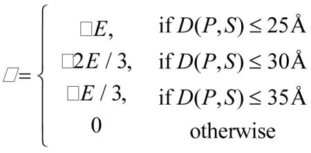(Equation 1)

We sum all ε for all probing experiments P and for all nucleotides S. The lower the energy is the better the fit is with the pairwise distance constraints. Here, we used the MPE data published by the Weeks’s group on the tRNA-ASP structure [12]. We assumed that the MPE profiles for the tRNA-ASP would be appropriate for the tRNA-VAL if we insert an extra dummy nucleotide in the variable loop of the tRNA-ASP profile, to match the sequence length of the tRNA-VAL.

MOHCA fitness

In the context of RNA modelling, MOHCA generates pairwise distance constraints, which we assign between pairs of C1’ backbone atoms. For each distance constraint, a squared penalty score, Δ², is given for any distance d beyond 30 Å; Δ = (d - 30). Hence, the fit of a model is the sum of its penalties. Since MC-Sym does not make use of internal energy, then there is no need for a coupling constant between the MOHCA distance violations and the energy of a structure. Here, we used the distance constraints from the native state of the P4-P6 domain [13].

The difference in the interpretation of the EDTA-based distance data between MPE and MOHCA prompted us to reinterpret the MPE. For MPE, the models are gratified for their fit to various distance constraints proportionally to the cleavage intensity at the measured sites (Eq. 1), whereas in MOHCA, the cleavage intensities are not taken into account, and thus the models are penalised for distance violations from the estimated tether probe length. We thus reinterpreted the MPE data for the tRNA. As suggested by Han and Dervan [11], we determined a strong cleavage for that adjacent to *U, medium for that proximal to *U (in the range 11-24 Å), and very weak for that distal to *U (in the range > 40 Å) (Fig. S3).

SAXS fitness

Because of the high residency of water molecules in both the minor and major grooves [65], and the presence of counter-ions near the negatively charged phosphate groups, we developed a new and fast method that explicitly takes into account the scattering of the first hydration shells [66]. This method has been developed in collaboration with Drs. Yang and Roux at the University of Chicago, and is similar to the approach they developed for proteins [67]. In the modelling context, the theoretical and experimental scattering curves are compared. This is similar to using CRYSOL, but: 1) we explicitly takes into account the first hydration shells by soaking the 3-D model in a box of explicit water molecules whose scattering contribution is added to that of the molecule; and, 2) we approximate the scattering profile of the nucleotides by using a two pseudo-particle model, one for the backbone located at the O5′ atom (near the phosphate group and counter-ion), and another one located in the base. The scattering profiles of each nucleotide (A, C, G, and U) are encoded in a form factor and calibrated to reproduce best the experimental tRNA SAXS data. The increase in the number of scatterers (i.e. objects producing scattering) by the addition of explicit water is counter balanced by the reduction of scatterers in the 3D model, and thus allowing for a fast SAXS fitness evaluation despite the many more atoms to be considered. The scattering is evaluated by the Debye formula [68]. We previously studied in details the use of SAXS data to reproduce a tRNA and P4-P6 domain [66]. Here, we used the SAXS data provided by the Bax’s laboratory for the tRNA [30], and the SAXS data from the Doniach’s laboratory for the P4-P6 domain [23].

Normalized Z-score

To express the fitness of a model to various experimental data types, we first compute a normalised Z-score, Ze(x), for the fitness of the model x in an experiment type e. Then, the total fit, Z(x), is simply given by ∑_e Z_e (x·) The Z-score, Z(x) = (x–μ)/σ, takes into account the mean, μ, and the standard deviation, σ, of the fits of all models for each experiment type. The normalised Z-score is $Z_e\left(x\right)=(Z_e\left(x\right)-Z_e^{\min })∕(Z_e^{\max }-Z_e^{\min })$, so that each experimental data type contribution is between zero and one, where one signifies the best fit (care is taken to properly compute Z_e(x) given that the highest or lowest experimental fit value is the best).

Global distance test (GDT-TS)

We optimally superimpose a predicted 3-D structure on the native structure. Then, we count the number of heavy atoms in the model that are within 1, 2, 4, and 8 Å of RMSD (all atoms) between the prediction and the native structure, which we divide by four times the number of atoms. For a perfect prediction, all N atoms would be within respectively 1, 2, 4, and 8 Å of RMSD, and thus the GDT-TS = (N + N + N + N) / 4N = 1. For a very bad model none of the atoms would be within 8 Å (and thus neither within 4, 2 nor 1 Å), and thus the GDT-TS = 0. The GDT-TS score is a measure of similarity between two 3-D structures on a scale between 0 (little similarity) and 1 (identical structures).

Model selection procedure

A question that naturally arises is how can we select a few representative structures that best fit the experimental data. Declaring the best-fit model as the native fold is dangerous because many models fit the data. Therefore, we sort the models from best to worst fit based on their normalized Z-score (see above), and we choose the top N models, where N is picked randomly between 100 and 500. We define this set as promising, and we partition it into 10 subsets using the K-clustering algorithm based on RMSD. We expect the K-clustering (K=10) to yield subsets of 10 to 50 members each. We choose the centroid of each subset, which on average fits best the experimental data. We define this model as the representative of the native fold. Because of the stochastic nature of the greedy K-clustering method, this selection procedure is repeated a hundred times and we report the averaged RMSD and Global Distance Test (GDT-TS [43,44]) between the centroids and their corresponding reference structures.

Supplementary Material

01

Figure S1. Discriminative power of experimental data on tRNA. (Top) Low set. (Bottom) High set. ad) Hydroxyl radical footprinting (OH); high values better (indicated by the ‘+’ sign). be) Methidiumpropyl-EDTA (MPE); low values better (indicated by the ‘+’ sign). cf) Small-angle X-ray scattering (SAXS); low values better (indicated by the ‘+’ sign).

02

Figure S2. Discriminative power of experimental data on P4-P6. (Top) Low set. (Bottom) High set. ad) Hydroxyl radical footprinting (OH); high values better (indicated by the ‘+’ sign). be) Multiplexed hydroxyl radical cleavage analysis (MOHCA); low values better (indicated by the ‘+’ sign). cf) Small-angle X-ray scattering (SAXS); low values better (indicated by the ‘+’ sign).

03

Figure S3. Reinterpretation of MPE data for tRNA. Distances that are over 30 Å (MPE*) are shown on the top row; those over 35 Å (MPE**) on the bottom row. A quadratic penalty function Δ² is applied to the low (left) and high (right) sets. Any site with a cleavage intensity ratio I/<I> above 1.0 should be within 30 Å of the probe’s base. The distanceover 30 Å, Δ=(d - 30),is scored as Δ² for MPE* (Δ=(d - 35)for MPE**). Lower values are better. A 3-D structure that has all experimentally probed distances within the probe’s reach will have an MPE score of 0 (i.e. no distance violation). This interpretation differs from that of Figure S1, where the cleavage intensities were converted to pseudo-energies in an intensity-dependent fashion.

References

- 1.Sharp PA. The centrality of RNA. Cell. 2009;136:577–580. doi: 10.1016/j.cell.2009.02.007. [DOI] [PubMed] [Google Scholar]
- 2.Crick F. Central dogma of molecular biology. Nature. 1970;227:561–563. doi: 10.1038/227561a0. [DOI] [PubMed] [Google Scholar]
- 3.Parisien M, Major F. The MC-Fold and MC-Sym pipeline infers RNA structure from sequence data. Nature. 2008;452:51–55. doi: 10.1038/nature06684. [DOI] [PubMed] [Google Scholar]
- 4.Das R, Baker D. Automated de novo prediction of native-like RNA tertiary structures. Proc Natl Acad Sci U S A. 2007;104:14664–14669. doi: 10.1073/pnas.0703836104. [DOI] [PMC free article] [PubMed] [Google Scholar]
- 5.Ding F, Sharma S, Chalasani P, Demidov VV, Broude NE, et al. Ab initio RNA folding by discrete molecular dynamics: from structure prediction to folding mechanisms. Rna. 2008;14:1164–1173. doi: 10.1261/rna.894608. [DOI] [PMC free article] [PubMed] [Google Scholar]
- 6.Jonikas MA, Radmer RJ, Laederach A, Das R, Pearlman S, et al. Coarse-grained modeling of large RNA molecules with knowledge-based potentials and structural filters. RNA. 2009;15:189–199. doi: 10.1261/rna.1270809. [DOI] [PMC free article] [PubMed] [Google Scholar]
- 7.Martinez HM, Maizel JV, Jr., Shapiro BA. RNA2D3D: a program for generating, viewing, and comparing 3-dimensional models of RNA. J Biomol Struct Dyn. 2008;25:669–683. doi: 10.1080/07391102.2008.10531240. [DOI] [PMC free article] [PubMed] [Google Scholar]
- 8.Draper DE, Grilley D, Soto AM. Ions and RNA folding. Annu Rev Biophys Biomol Struct. 2005;34:221–243. doi: 10.1146/annurev.biophys.34.040204.144511. [DOI] [PubMed] [Google Scholar]
- 9.Williamson JR. Induced fit in RNA-protein recognition. Nature Structural Biology. 2000;7:834–837. doi: 10.1038/79575. [DOI] [PubMed] [Google Scholar]
- 10.Tullius TD, Greenbaum JA. Mapping nucleic acid structure by hydroxyl radical cleavage. Curr Opin Chem Biol. 2005;9:127–134. doi: 10.1016/j.cbpa.2005.02.009. [DOI] [PubMed] [Google Scholar]
- 11.Han H, Dervan PB. Visualization of RNA tertiary structure by RNA-EDTA.Fe(II) autocleavage: analysis of tRNA(Phe) with uridine-EDTA.Fe(II) at position 47. Proc Natl Acad Sci U S A. 1994;91:4955–4959. doi: 10.1073/pnas.91.11.4955. [DOI] [PMC free article] [PubMed] [Google Scholar]
- 12.Gherghe CM, Leonard CW, Ding F, Dokholyan NV, Weeks KM. Native-like RNA tertiary structures using a sequence-encoded cleavage agent and refinement by discrete molecular dynamics. J Am Chem Soc. 2009;131:2541–2546. doi: 10.1021/ja805460e. [DOI] [PMC free article] [PubMed] [Google Scholar]
- 13.Das R, Kudaravalli M, Jonikas M, Laederach A, Fong R, et al. Structural inference of native and partially folded RNA by high-throughput contact mapping. Proc Natl Acad Sci U S A. 2008;105:4144–4149. doi: 10.1073/pnas.0709032105. [DOI] [PMC free article] [PubMed] [Google Scholar]
- 14.Latham JA, Cech TR. Defining the inside and outside of a catalytic RNA molecule. Science. 1989;245:276–282. doi: 10.1126/science.2501870. [DOI] [PubMed] [Google Scholar]
- 15.Mitra S, Shcherbakova IV, Altman RB, Brenowitz M, Laederach A. High-throughput single-nucleotide structural mapping by capillary automated footprinting analysis. Nucleic Acids Res. 2008;36:e63. doi: 10.1093/nar/gkn267. [DOI] [PMC free article] [PubMed] [Google Scholar]
- 16.Mortimer SA, Weeks KM. A fast-acting reagent for accurate analysis of RNA secondary and tertiary structure by SHAPE chemistry. J Am Chem Soc. 2007;129:4144–4145. doi: 10.1021/ja0704028. [DOI] [PubMed] [Google Scholar]
- 17.Merino EJ, Wilkinson KA, Coughlan JL, Weeks KM. RNA structure analysis at single nucleotide resolution by selective 2′-hydroxyl acylation and primer extension (SHAPE) J Am Chem Soc. 2005;127:4223–4231. doi: 10.1021/ja043822v. [DOI] [PubMed] [Google Scholar]
- 18.Deigan KE, Li TW, Mathews DH, Weeks KM. Accurate SHAPE-directed RNA structure determination. Proc Natl Acad Sci U S A. 2009;106:97–102. doi: 10.1073/pnas.0806929106. [DOI] [PMC free article] [PubMed] [Google Scholar]
- 19.Wilkinson KA, Gorelick RJ, Vasa SM, Guex N, Rein A, et al. High-throughput SHAPE analysis reveals structures in HIV-1 genomic RNA strongly conserved across distinct biological states. PLoS Biol. 2008;6:e96. doi: 10.1371/journal.pbio.0060096. [DOI] [PMC free article] [PubMed] [Google Scholar]
- 20.Wang Z, Parisien M, Scheets K, Miller WA. The cap-binding translation initiation factor, eIF4E, binds a pseudoknot in a viral cap-independent translation element. Structure. 2011;19:868–880. doi: 10.1016/j.str.2011.03.013. [DOI] [PMC free article] [PubMed] [Google Scholar]
- 21.Reymond C, Levesque D, Bisaillon M, Perreault JP. Developing three-dimensional models of putative-folding intermediates of the HDV ribozyme. Structure. 2010;18:1608–1616. doi: 10.1016/j.str.2010.09.024. [DOI] [PMC free article] [PubMed] [Google Scholar]
- 22.Kim J, Yu S, Shim B, Kim H, Min H, et al. A robust peak detection method for RNA structure inference by high-throughput contact mapping. Bioinformatics. 2009;25:1137–1144. doi: 10.1093/bioinformatics/btp110. [DOI] [PubMed] [Google Scholar]
- 23.Lipfert J, Doniach S. Small-angle X-ray scattering from RNA, proteins, and protein complexes. Annual Review of Biophysics and Biomolecular Structure. 2007;36:307–327. doi: 10.1146/annurev.biophys.36.040306.132655. [DOI] [PubMed] [Google Scholar]
- 24.Lipfert J, Chu VB, Bai Y, Herschlag D, Doniach S. Low-Resolution Models for Nucleic Acids from Small-Angle X-ray Scattering with Applications to Electrostatic Modeling. Journal of Applied Crystallography. 2007;40:s229–s234. [Google Scholar]
- 25.Ali M, Lipfert J, Seifert S, Herschlag D, Doniach S. The ligand-free state of the TPP riboswitch: a partially folded RNA structure. J Mol Biol. 2010;396:153–165. doi: 10.1016/j.jmb.2009.11.030. [DOI] [PMC free article] [PubMed] [Google Scholar]
- 26.Koch MH, Vachette P, Svergun DI. Small-angle scattering: a view on the properties, structures and structural changes of biological macromolecules in solution. Q Rev Biophys. 2003;36:147–227. doi: 10.1017/s0033583503003871. [DOI] [PubMed] [Google Scholar]
- 27.Svergun D, Barberato C, Koch MHJ. CRYSOL - A program to evaluate x-ray solution scattering of biological macromolecules from atomic coordinates. Journal of Applied Crystallography. 1995;28:768–773. [Google Scholar]
- 28.Svergun DI. Restoring low resolution structure of biological macromolecules from solution scattering using simulated annealing (vol 76, pg 2879, 1999) Biophysical Journal. 1999;77:2896–2896. doi: 10.1016/S0006-3495(99)77443-6. [DOI] [PMC free article] [PubMed] [Google Scholar]
- 29.Svergun DI, Semenyuk AV, Feigin LA. Small-Angle-Scattering-Data Treatment by the Regularization Method. Acta Crystallographica Section A. 1988;44:244–250. [Google Scholar]
- 30.Grishaev A, Ying J, Canny MD, Pardi A, Bax A. Solution structure of tRNAVal from refinement of homology model against residual dipolar coupling and SAXS data. J Biomol NMR. 2008;42:99–109. doi: 10.1007/s10858-008-9267-x. [DOI] [PMC free article] [PubMed] [Google Scholar]
- 31.Cate JH, Gooding AR, Podell E, Zhou KH, Golden BL, et al. Crystal structure of a group I ribozyme domain: Principles of RNA packing. Science. 1996;273:1678–1685. doi: 10.1126/science.273.5282.1678. [DOI] [PubMed] [Google Scholar]
- 32.Major F, Gautheret D, Cedergren R. Reproducing the three-dimensional structure of a tRNA molecule from structural constraints. Proc Natl Acad Sci U S A. 1993;90:9408–9412. doi: 10.1073/pnas.90.20.9408. [DOI] [PMC free article] [PubMed] [Google Scholar]
- 33.Major F, Turcotte M, Gautheret D, Lapalme G, Fillion E, et al. The combination of symbolic and numerical computation for three-dimensional modeling of RNA. Science. 1991;253:1255–1260. doi: 10.1126/science.1716375. [DOI] [PubMed] [Google Scholar]
- 34.Major F. Building three-dimensional ribonucleic acid structures. Computing in Science & Engineering. 2003;5:44–53. [Google Scholar]
- 35.Lemieux S, Major F. Automated extraction and classification of RNA tertiary structure cyclic motifs. Nucleic Acids Res. 2006;34:2340–2346. doi: 10.1093/nar/gkl120. [DOI] [PMC free article] [PubMed] [Google Scholar]
- 36.Jonikas MA, Radmer RJ, Altman RB. Knowledge-based instantiation of full atomic detail into coarse-grain RNA 3D structural models. Bioinformatics. 2009;25:3259–3266. doi: 10.1093/bioinformatics/btp576. [DOI] [PMC free article] [PubMed] [Google Scholar]
- 37.Sharma S, Ding F, Dokholyan NV. iFoldRNA: three-dimensional RNA structure prediction and folding. Bioinformatics. 2008;24:1951–1952. doi: 10.1093/bioinformatics/btn328. [DOI] [PMC free article] [PubMed] [Google Scholar]
- 38.Cao S, Chen SJ. Physics-based de novo prediction of RNA 3D structures. The journal of physical chemistry. 2011;115:4216–4226. doi: 10.1021/jp112059y. [DOI] [PMC free article] [PubMed] [Google Scholar]
- 39.Sim AY, Levitt M. Clustering to identify RNA conformations constrained by secondary structure. Proc Natl Acad Sci U S A. 2011;108:3590–3595. doi: 10.1073/pnas.1018653108. [DOI] [PMC free article] [PubMed] [Google Scholar]
- 40.Levitt M. Detailed molecular model for transfer ribonucleic acid. Nature. 1969;224:759–763. doi: 10.1038/224759a0. [DOI] [PubMed] [Google Scholar]
- 41.Klingler TM, Brutlag DL. Detection of correlations in tRNA sequences with structural implications. Proc Int Conf Intell Syst Mol Biol. 1993;1:225–233. [PubMed] [Google Scholar]
- 42.Costa M, Michel F. Frequent Use of the Same Tertiary Motif by Self-Folding Rnas. Embo Journal. 1995;14:1276–1285. doi: 10.1002/j.1460-2075.1995.tb07111.x. [DOI] [PMC free article] [PubMed] [Google Scholar]
- 43.Zemla A, Venclovas C, Moult J, Fidelis K. Processing and analysis of CASP3 protein structure predictions. Proteins-Structure Function and Genetics. 1999:22–29. doi: 10.1002/(sici)1097-0134(1999)37:3+<22::aid-prot5>3.3.co;2-n. [DOI] [PubMed] [Google Scholar]
- 44.Ginalski K, Grishin NV, Godzik A, Rychlewski L. Practical lessons from protein structure prediction. Nucleic Acids Research. 2005;33:1874–1891. doi: 10.1093/nar/gki327. [DOI] [PMC free article] [PubMed] [Google Scholar]
- 45.Nilsson L, Rigler R, Laggner P. Structural variability of tRNA: small-angle x-ray scattering of the yeast tRNAphe-Escherichia coli tRNAGlu2 complex. Proc Natl Acad Sci U S A. 1982;79:5891–5895. doi: 10.1073/pnas.79.19.5891. [DOI] [PMC free article] [PubMed] [Google Scholar]
- 46.Fang X, Littrell K, Yang XJ, Henderson SJ, Siefert S, et al. Mg2+-dependent compaction and folding of yeast tRNAPhe and the catalytic domain of the B. subtilis RNase P RNA determined by small-angle X-ray scattering. Biochemistry. 2000;39:11107–11113. doi: 10.1021/bi000724n. [DOI] [PubMed] [Google Scholar]
- 47.Lemieux S, Chartrand P, Cedergren R, Major F. Modeling active RNA structures using the intersection of conformational space: application to the lead-activated ribozyme. RNA. 1998;4:739–749. doi: 10.1017/s1355838298971266. [DOI] [PMC free article] [PubMed] [Google Scholar]
- 48.Laing C, Schlick T. Computational approaches to 3D modeling of RNA. Journal of Physics-Condensed Matter. 2010;22 doi: 10.1088/0953-8984/22/28/283101. [DOI] [PMC free article] [PubMed] [Google Scholar]
- 49.Chu VB, Lipfert J, Bai Y, Pande VS, Doniach S, et al. Do conformational biases of simple helical junctions influence RNA folding stability and specificity? RNA. 2009;15:2195–2205. doi: 10.1261/rna.1747509. [DOI] [PMC free article] [PubMed] [Google Scholar]
- 50.Bailor MH, Sun X, Al-Hashimi HM. Topology links RNA secondary structure with global conformation, dynamics, and adaptation. Science. 2010;327:202–206. doi: 10.1126/science.1181085. [DOI] [PubMed] [Google Scholar]
- 51.Bailor MH, Mustoe AM, Brooks CL, 3rd, Al-Hashimi HM. Topological constraints: using RNA secondary structure to model 3D conformation, folding pathways, and dynamic adaptation. Curr Opin Struct Biol. 2011;21:296–305. doi: 10.1016/j.sbi.2011.03.009. [DOI] [PMC free article] [PubMed] [Google Scholar]
- 52.Lee JC, Cannone JJ, Gutell RR. The lonepair triloop: a new motif in RNA structure. J Mol Biol. 2003;325:65–83. doi: 10.1016/s0022-2836(02)01106-3. [DOI] [PubMed] [Google Scholar]
- 53.Zhuang Z, Jaeger L, Shea JE. Probing the structural hierarchy and energy landscape of an RNA T-loop hairpin. Nucleic Acids Res. 2007;35:6995–7002. doi: 10.1093/nar/gkm719. [DOI] [PMC free article] [PubMed] [Google Scholar]
- 54.Bouchard P, Lacroix-Labonte J, Desjardins G, Lampron P, Lisi V, et al. Role of SLV in SLI substrate recognition by the Neurospora VS ribozyme. Rna-a Publication of the Rna Society. 2008;14:736–748. doi: 10.1261/rna.824308. [DOI] [PMC free article] [PubMed] [Google Scholar]
- 55.Krasilnikov AS, Mondragon A. On the occurrence of the T-loop RNA folding motif in large RNA molecules. Rna. 2003;9:640–643. doi: 10.1261/rna.2202703. [DOI] [PMC free article] [PubMed] [Google Scholar]
- 56.Fuller W, Hodgson A. Conformation of the anticodon loop in tRNA. Nature. 1967;215:817–821. doi: 10.1038/215817a0. [DOI] [PubMed] [Google Scholar]
- 57.Tyagi R, Mathews DH. Predicting helical coaxial stacking in RNA multibranch loops. Rna. 2007;13:939–951. doi: 10.1261/rna.305307. [DOI] [PMC free article] [PubMed] [Google Scholar]
- 58.Cate JH, Gooding AR, Podell E, Zhou K, Golden BL, et al. RNA tertiary structure mediation by adenosine platforms. Science. 1996;273:1696–1699. doi: 10.1126/science.273.5282.1696. [DOI] [PubMed] [Google Scholar]
- 59.Jaeger L, Verzemnieks EJ, Geary C. The UA_handle: a versatile submotif in stable RNA architectures. Nucleic Acids Res. 2009;37:215–230. doi: 10.1093/nar/gkn911. [DOI] [PMC free article] [PubMed] [Google Scholar]
- 60.Michel F, Westhof E. Modelling of the three-dimensional architecture of group I catalytic introns based on comparative sequence analysis. J Mol Biol. 1990;216:585–610. doi: 10.1016/0022-2836(90)90386-Z. [DOI] [PubMed] [Google Scholar]
- 61.Murphy FL, Cech TR. Gaaa Tetraloop and Conserved Bulge Stabilize Tertiary Structure of a Group-I Intron Domain. Journal of Molecular Biology. 1994;236:49–63. doi: 10.1006/jmbi.1994.1117. [DOI] [PubMed] [Google Scholar]
- 62.Jaeger L, Michel F, Westhof E. Involvement of a Gnra Tetraloop in Long-Range Tertiary Interactions. Journal of Molecular Biology. 1994;236:1271–1276. doi: 10.1016/0022-2836(94)90055-8. [DOI] [PubMed] [Google Scholar]
- 63.Sanner MF, Olson AJ, Spehner JC. Reduced surface: an efficient way to compute molecular surfaces. Biopolymers. 1996;38:305–320. doi: 10.1002/(SICI)1097-0282(199603)38:3%3C305::AID-BIP4%3E3.0.CO;2-Y. [DOI] [PubMed] [Google Scholar]
- 64.Takamoto K, Das R, He Q, Doniach S, Brenowitz M, et al. Principles of RNA compaction: Insights from the equilibrium folding pathway of the P4-P6 RNA domain in monovalent cations. Journal of Molecular Biology. 2004;343:1195–1206. doi: 10.1016/j.jmb.2004.08.080. [DOI] [PubMed] [Google Scholar]
- 65.Auffinger P, Hashem Y. Nucleic acid solvation: from outside to insight. Current Opinion in Structural Biology. 2007;17:325–333. doi: 10.1016/j.sbi.2007.05.008. [DOI] [PubMed] [Google Scholar]
- 66.Yang S, Parisien M, Major F, Roux B. RNA structure determination using SAXS data. J Phys Chem B. 2010;114:10039–10048. doi: 10.1021/jp1057308. [DOI] [PMC free article] [PubMed] [Google Scholar]
- 67.Yang SC, Park S, Makowski L, Roux B. A Rapid Coarse Residue-Based Computational Method for X-Ray Solution Scattering Characterization of Protein Folds and Multiple Conformational States of Large Protein Complexes. Biophysical Journal. 2009;96:4449–4463. doi: 10.1016/j.bpj.2009.03.036. [DOI] [PMC free article] [PubMed] [Google Scholar]
- 68.Debye P. Dispersion of Rontgen rays. Annalen der Physik. 1915;46:809–823. [Google Scholar]
Associated Data
This section collects any data citations, data availability statements, or supplementary materials included in this article.
Supplementary Materials