fMRI-DTI modeling via landmark distance atlases for prediction and detection of fiber tracts

Abstract

The overall goal of this research is the design of statistical atlas models that can be created from normal subjects, but may generalize to be applicable to abnormal brains. We present a new style of joint modeling of fMRI, DTI, and structural MRI. Motivated by the fact that a white matter tract and related cortical areas are likely to displace together in the presence of a mass lesion (brain tumor), in this work we propose a rotation and translation invariant model that represents the spatial relationship between fiber tracts and anatomic and functional landmarks. This landmark distance model provides a new basis for representation of fiber tracts and can be used for detection and prediction of fiber tracts based on landmarks. Our results indicate that the measured model is consistent across normal subjects, and thus suitable for atlas building. Our experiments demonstrate that the model is robust to displacement and missing data, and can be successfully applied to a small group of patients with mass lesions.

Introduction

Typically, the clinical interpretation of complex white matter tractography data is undertaken in an interactive fashion, where tracts of interest are selected by an expert. This has inspired the development of automatic methods that identify tracts based on a white matter atlas, a standardized anatomic model. Individualization of atlas information, or the application of standardized anatomic models to specific subjects, is a non-trivial problem that has been addressed using sophisticated image registration and segmentation methods (Fischl et al., 2002; Hagler et al., 2009; Hua et al., 2008b; Pohl et al., 2006). However, these methods may not generalize well to neurosurgical patients with mass lesions due to the difficulty of aligning a voxelbased atlas to an individual patient. Thus atlases based on the normal anatomy of the fiber tracts may not be applicable to displaced or otherwise pathological tracts. Instead of a more traditional voxel-based atlas that is represented in an absolute coordinate system, we propose to develop a new style of relative model that does not employ absolute coordinates. The motivation behind the proposed relative model is to represent anatomic relationships that may be preserved despite displacement due to mass lesions.

It has long been known that characteristic spatial relationships exist between anatomic and functional landmarks and white matter (WM) fiber tracts. For example, the corticospinal tract runs from the motor cortex to the middle third of the cerebral peduncle (Holodny et al., 2005), and the arcuate fasciculus connects frontal and temporal language areas (Glasser and Rilling, 2008). These classical anatomic relationships have been used for interactive identification of fiber tracts using anatomic and functional landmarks in individual healthy subjects (Mori et al., 2005) and in surgical patients (Kamada et al., 2005; Schonberg et al., 2006). Automation of this process, using spatial volumetric models to define anatomic landmarks, was performed in both healthy subjects and surgical patients (Zhang et al., 2008). In tumor patients, it has been suggested that fMRI activations are superior to anatomically defined regions of interest for selecting tracts (Schonberg et al., 2006) due to the fact that a WM tract and related cortical areas are likely to displace together. Overall, the body of related work indicates that the spatial relationships between fiber tracts, functional activations, and anatomic regions of interest are not only stable across healthy subjects, but that they are relatively preserved in surgical patients.

We propose to explicitly build a model of such spatial relationships. Specifically, our proposed landmark distance model is a feature vector describing the distances between fiber tract trajectories and points that represent functional and structural landmarks. Themultimodality input data used to construct the model includes diffusion tensor magnetic resonance imaging (DTI), functional magnetic resonance imaging (fMRI), and structural magnetic resonance imaging (structural MRI).

We are unaware of any studies similar to our current approach, however other groups have proposed methods for modeling fMRI and DTI, separately and together, in the human brain. Various types of voxel-based DTI atlases and trajectory-based DTI fiber tract atlases have been proposed (e.g. Mori et al. (2005); Goodlett et al. (2006); O’Donnell and Westin (2007); Hua et al. (2008b); Catani and de Schotten (2008); Maddah et al. (2008); Mori et al. (2008); Yushkevich et al. (2008); Hagler et al. (2009)). The gray–white matter interface has been modeled using spatial probability maps of DTI fiber tract terminations over cortical areas (Hua et al., 2008a). fMRI activations have generally been modeled as voxel maps (Worsley and Friston, 1995), but modeling of fMRI activation locations as points has been proposed, and the relationship of such points to nearby cortical sulci has been assessed using a triangulation approach (Tucholka et al., 2008). Joint fMRI-DTI relationships have been modeled using matrices of functional and structural connectivity, without incorporating spatial information (Gong et al., 2009; Greicius et al., 2009; Skudlarski et al., 2008; Venkataraman et al., 2010). In the anthropology literature, spatial relationships between landmarks have been modeled as pairwise distances (Lele and Richtsmeier, 1991).

In contrast to previous work, we propose to build a quantitative model of structural–functional spatial relationships in the brain. The main contribution of this work is the landmark distance (LD) model, a new style of joint modeling of fMRI, DTI, and structural MRI. We show that the LD model can be used to predict and detect fiber trajectories, and can be robust to displacement. Finally we test the model in several patients with abnormal anatomy. In this work we further develop ideas first presented in a conference workshop (O’Donnell et al., 2009a). Relative to our earlier work, the current paper improves the prediction method, introduces the concept of tract detection based on the model, and presents results in patients with mass lesions.

Methods

Acquisition and data processing

Five healthy control right-handed subjects (3 female, 2 male, mean age 26.8±2.77 standard deviation) and 3 patients with brain tumors near motor and/or language areas were studied. Written informed consent was obtained from all subjects in accordance with protocols set forth by Partners Healthcare Institutional Review Board. Imaging was acquired with a 3T GE Signa system as follows. fMRI (EPI with single channel head coil, TR=2000 ms, TE=40 ms, flip angle=90, FOV=25.6 cm, matrix=80×80, 27 axial slices, voxel size=3.2×3.2×4 mm³) was acquired during the following tasks: antonym generation, noun categorization, left and right hand clench, left and right foot toe wiggle, and lip pursing. Structural (whole brain SPGR, or Spoiled Gradient Recalled Acquisition in Steady State) and diffusion weighted images (EPI with 8 channel head coil and ASSET, TR=14,000 ms, TE=74.9 ms, b value=1000 s/mm², 51 gradient directions, 2 baseline images, FOV=25.6 cm, 128×128 matrix, voxel size 2×2×2.6 mm³) were acquired. The neurosurgical patients were studied with clinical protocols that were similar but had reduced scanning time.

An input dataset including fiber tracts and anatomic and functional landmarks was created from the 5 normal subjects as follows. White matter tracts of interest (arcuate fasciculus or AF and corticospinal tract or CST) were automatically segmented in the controls using a high-dimensional atlas (O’Donnell and Westin, 2007). This pipeline included several steps: Whole-brain tractography (Runge–Kutta order two streamline tractography) was seeded in the entire white matter of each subject. DTI-derived FA images were affinely registered in 3D Slicer (www.slicer.org) to the atlas mean FA image, and this transform was applied to the tractography. Each “fiber” was then labeled based on trajectory similarity to atlas fiber clusters (O’Donnell and Westin, 2007). After tract labeling, the fibers were reverse-transformed back into subject space.

Statistical Parametric Mapping (SPM) was used to process functional data (www.fil.ion.ucl.ac.uk/spm/). Motion correction was performed via image realignment, then each dataset was coregistered to the individual subject’s anatomical MRI (SPGR). Data were analyzed using the general linear model, a hemodynamic response function (HRF) was produced based on each task paradigm, and statistical parametric maps were then created based on the T score correlation between the HRF and voxel by voxel BOLD signal. Given the individual differences in BOLD signal intensity and statistical significance levels, interactive expert evaluation for optimization of fMRI activations (Håberg et al., 2004; O’Shea et al., 2006) is the standard for presurgical fMRI mapping. Interactive fMRI thresholding was performed for each subject, and an individually determined threshold was selected that resulted in activation in the anatomical region(s) known to be associated with each task.

Anatomical and functional landmarks were selected manually using 3D Slicer (Fig. 1). Ten fMRI activation peaks (vision, hand, foot, and lip motor for each hemisphere, and putative Broca’s and Wernicke’s areas) and five anatomic landmarks from the SPGR images (in anterior/posterior corpus callosum in midsagittal plane, anterior commissure, and cerebral peduncles) were selected for each normal subject (Tables 1 and 2). For within-subject coregistration of multiple modalities, each subject’s fMRI activation peaks and anatomic landmarks were registered to the DTI space by affine registration of the SPGR to the subject’s FA image.

Fig. 1.

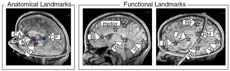
Anatomical landmarks (corpus callosum, anterior commisure, and cerebral peduncle) and functional landmarks (motor, language, and visual activation peaks) from control subject 1. Arrows label each landmark with its acronym (see Tables 1 and 2). Spheres centered at each landmark have been annotated with stars to improve visibility.

Table 1.

Acronyms for anatomic and functional landmarks in the left and right hemispheres, LHem and RHem. These subjects had left-lateralized language, so Broca and Wernicke’s areas are in the left hemisphere. The crossing of the pyramidal (CST) tract means that right hand (RH) motor activation is in the left hemisphere, and so on. The lip pursing activation is bilateral, so face left (FL) is the activation in the left hemisphere.

Left hem. landmark	Right Hem. landmark	Description
VL (vision left)	VR (vision right)	Vision fMRI
RH (right hand)	LH (left hand)	Hand fMRI
RF (right foot)	LF (left foot)	Foot fMRI
FL (face left)	FR (face right)	Lip pursing fMRI
BL (Broca left)		Putative Broca fMRI
WL (Wernicke left)		Putative Wernicke fMRI
PL (peduncle Left)	PR (peduncle right)	Cerebral peduncle

Table 2.

Acronyms for anatomic landmarks in the midsagittal plane.

Midsagittal Landmark	Description
AC	Anterior commissure
CA	Anterior corpus callosum
CP	Posterior corpus callosum

The selected tracts and the fMRI activations and landmark points from all normal subjects were then loaded into Matlab (The Math-Works, Inc.), providing a dataset for construction of the LD model (Fig. 2). Note that due to the properties of the LD model (Measurement of the landmark distance model section), it was not necessary to register across subjects, so these tracts and landmarks were represented in each individual’s subject-specific coordinate system.

Fig. 2.

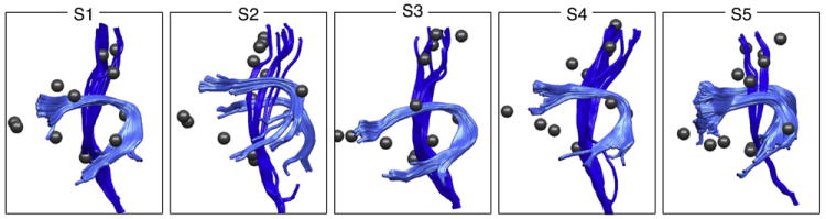
Input dataset from 5 subjects including arcuate fasciculus (AF, light blue); left and right corticospinal tracts (CST, dark blue); and fMRI activation peaks plus anatomic landmarks (spheres).

The data from the 3 patients were also processed by performing seeding of whole-brain tractography, fMRI processing, and manual selection of all possible landmarks based on available fMRI and anatomical data. These steps were performed as described above. Note that due to the properties of the LD model, it was not necessary to register the atlas to the patient data or vice versa, so all steps were performed in the patient-specific coordinate system.

Measurement of the landmark distance model

The LD model is a rotation-invariant and translation-invariant representation of spatial relationships betweenWMtracts and functional and structural landmarks. Measurement of the model is straightforward and consists of two steps.

In the first step, each fiber is converted to an intermediate representation that can handle fibers of varying lengths. This representation uses a fixed number of points, with variable inter-point distance, to represent fibers of varying lengths. Each fiber’s interpoint distance is determined by the length of the fiber, in order to space the points evenly along the fiber. This gives a fixed-length vector of points (i.e. 10 points, or 30 points along the fiber) that represents each fiber, regardless of the length of the fiber.

Then in the second step, the LD model is calculated from this fixed-length fiber representation. For each point along the fiber, the distance is measured to a functional or structural landmark (Fig. 3). By measuring distances to multiple landmarks, the full LD model is constructed. By concatenating all distances into one vector, the LD model can be expressed as a vector of length f×l, where f is the number of points on the fiber and l is the number of landmarks. The distances in the LD model can be thought of in two ways: as a new basis for describing a fiber trajectory, and as a feature vector whose pattern identifies the fiber tract. Thus the LD model has two possible uses: prediction and detection of fiber tracts.

Fig. 3.

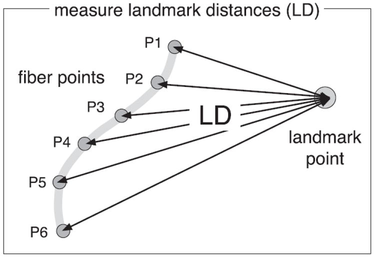
A 2D example demonstrating measurement of the LD model for a single fiber and a single landmark. The fiber is represented by a fixed number of points along the trajectory (6 points in this example, P1 to P6), then distances (arrows labeled LD) are measured from each point to the landmark.

Fiber prediction

For prediction of fiber tracts, the LD representation can be used as a generative model: given a new set of landmarks, a fiber trajectory can be predicted based on the known landmark distances from the model. The reverse is also true: given a fiber and the corresponding model of expected distances, fMRI landmarks can be estimated. In this way our method gives one possible alternative basis for representation of fiber tracts.

To predict the locations of points along fiber tracts, we use trilateration, the process of calculating an unknown point based on its distances to three or more known points. It can be thought of as finding the intersection of spheres centered at the known points with radii corresponding to the given distances (Fig. 4). The method is different from triangulation which uses a fixed baseline distance and two angles, though the terms triangulation and trilateration are sometimes used interchangeably.

Fig. 4.

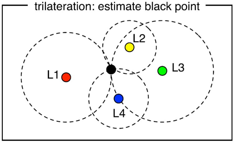
Method for fiber prediction based on the LD model. Estimation of a point’s coordinates based on its distance from 3 or more other points is called trilateration and is used in GPS systems. The desired distance from each input landmark point (L1–L4) gives the radius of each dashed circle. The circles converge on a black point that is the correct distance from all landmark points. We use this method to estimate the locations of points along a fiber trajectory, based on the given landmark locations and distances in the LD model.

When distances are known to more than three points, the solution to a trilateration problem can be found using nonlinear least squares. In our case, this minimizes the errors between the landmark distance model and the distances resulting from the current position of the unknown point x. To find x, the sum of squared errors r_i in distance to all known landmark points L_i is minimized. Each error r_i is calculated as the difference between the expected (modeled) landmark distance (LD_i) from point x to landmark L_i, and the distance from the current estimate for x to the location of L_i in the subject.

$$\underset{x}{\mathit{argmin}}\sum r_i{(x)}^2$$ (1)

$$r_i(x)={\mathit{LD}}_i-\parallel x-L_i\parallel$$ (2)

In Matlab we implemented this process using the function lsqnonlin. Thus given functional/structural landmark locations, and distances from each landmark to all points along a fiber (contained in an LD model), the trajectory of the fiber could be predicted.

Fiber detection

For detection of fibers, it is useful to consider the LD information as a feature vector describing each fiber. The concatenation of all landmark distance measurements from one fiber gives an LD feature vector of length f×l for that fiber. In fact this vector is unique to that fiber trajectory, given the subject’s landmarks, because the fiber can be exactly recalculated using trilateration. We propose to take advantage of the distinctiveness of LD feature vectors to identify fibers of interest.

First, the structures of interest must be modeled by measuring a representative LD feature vector for each structure. We call this representation an LD atlas. Next, to identify a structure of interest in a novel subject, we propose to calculate the LD feature vectors of all fibers in the WM of the novel subject (using that subject’s tractography and landmarks), then compare each fiber’s LD feature vector to the structure’s representative LD feature vector in the atlas. In this way, the fibers that are most similar to the WM structures in the atlas can be identified. This can be expressed as a classifier, h, that indicates whether a fiber f belongs to a structure represented by an LD atlas. The decision is made on the basis of some distance function, d, that compares the LD feature vectors of the atlas structure and the fiber. If this distance is less than a threshold (set by the user, or chosen to return a certain number of fibers, etc.), then the fiber f is considered to be part of the structure.

$$h(f)=d({\mathit{LD}}_{\mathit{atlas}},{\mathit{LD}}_f)<\mathit{threshold}$$ (3)

Thus it is necessary to design a measure, d, that quantifies the similarity or dissimilarity (distance) between LD vectors, perhaps taking into account additional attributes of the LD atlas such as variances. Ideally, the measure we develop will be robust to the sort of displacement that can be caused by a mass lesion, to enable use of the atlas even in patients with displaced fiber tracts. To this end, in this work we have performed experiments comparing several possible distance measures for LD feature vectors, including variants of the squared difference measure and a correlation-based measure. See Application of atlas: fiber tract detection with displacement section for definitions of these proposed measures.

Features of the LD model

We describe some of the design features of the LD model.

Invariance to rotation and translation, and robustness to scaling or displacement

Because the LD representation is invariant to rotation and translation, no image registration is needed to compare LD feature vectors across subjects. Correspondence is instead obtained according to landmark correspondence. In our implementation, the ordering of the landmarks determines the ordering of the data in the feature vectors to be compared. Thus in this work no registration was needed to apply the LD atlas to the patient data, due to known landmark correspondence.

The LD representation itself is not invariant to scaling, however fiber detection via an appropriate similarity measure can be robust to scaling or displacement. The effect of a relatively larger or smaller brain size would be to increase or decrease the magnitude of the distances in the LD model. This would be reflected in a scaling of the LD feature vector curve, such that the entire curve would scale either upwards or downwards on the LD axis. Local brain scaling such as displacement would cause a variable scaling of the curve, rather than a constant upwards or downwards scale of the entire curve. Our experiments demonstrate that selection of a similarity measure that is somewhat insensitive to such changes in the curve can allow fiber detection despite scaling or displacement in the brain.

Insensitivity to missing data

The LD model can handle missing data (missing distances to one or more landmarks). This is a very likely scenario as most patients would be unlikely to have all possible fMRI scans. For fiber prediction, mathematically three or more landmarks are needed. For fiber detection, three landmarks are also needed to uniquely characterize the points along a fiber (however, conceptually even two landmarks could be useful, for example in a scenario where they correspond to the endpoints of the fiber of interest). For practical purposes, at least three landmarks are needed for prediction or detection, thus it is important for the model to handle the presence of only a subset of landmark data. The missing data is handled by using the subset of atlas data that corresponds to the available patient data. For example, the distance measure can compare a fiber’s LD feature vector to the corresponding subset of the LD feature vector data in the LD atlas.

Invariance to fiber point ordering

A fiber representation (trajectory) can equivalently start from either endpoint of the fiber. In order to compare the LD vectors from different fibers within and across subjects, we addressed the problem that some vectors were produced in reverse order from others. To simplify further processing, a reordering function was written to align all vectors with the first input vector (according to whether correlation with the first vector was higher in the original or reverse orders). This function reversed the order of each LD vector (within the region corresponding to each landmark) if needed. This function was used for all operations on LD vectors including finding the mean and standard deviation within and across subjects for atlas creation, and subtraction of vectors during comparison to the atlas.

Fixed-length representation

The initial conversion of each fiber to a fixed-length representation (using a fixed number of points equally spaced along its trajectory) enables measurement of fixed-length LD feature vectors across all fibers in the brain and across subjects. Note that this does not change the length of the fiber, it simply fixes the length of the vector of data describing the fiber. This simplifies the pointwise fiber correspondence problem to a simple ordering problem (see above). Other solutions to the problem of pointwise correspondence along fiber tracts have required computation of coordinate systems based on local fiber geometry or voxel-based atlases (e.g. Goodlett et al. (2006); Maddah et al. (2008); Yushkevich et al. (2008); O’Donnell et al. (2009b); Hagler et al. (2009)). The fixed-length representation feature is important for computational speed and for application to abnormal subjects where coordinate systems based on the traditional atlases may not generalize well.

Experiments

Using the input dataset (Fig. 2), four experiments were performed. First, the proposed landmark distance atlas model (the LDA) was measured using the normal subject dataset. Next, the LDA was used to predict the locations of fiber tracts, in a leave-one-out experiment. Then, the robustness of LDA tract detection measures was tested under conditions of synthetic displacement. Finally, to assess whether the LDA from normal controls was similar to the LD of patients, the atlas was applied to detect fiber tracts in the patients with mass lesions.

Results

Measurement of landmark distance atlas

For each of the five normal subjects, the LD was measured between all fibers (within AF and CST) and all 15 activation points and anatomic landmarks. Fig. 5 shows measurements from all fibers in one subject, while Figs. 6 and 7 display results across all five normal subjects. Results demonstrate that the model is consistent across normal subjects (for both nearby and more distant fMRI activations and anatomic landmarks) thus it is suitable for atlas building.

Fig. 5.

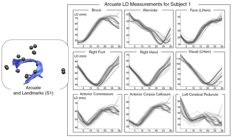
Measurement of landmark distances (LD) in subject 1, between left arcuate (AF) and nearby and distant landmarks. The plots on the right show LD measurements (dashed gray lines) from every fiber in the AF (shown at left in light blue), plus the mean LD in the whole structure (solid black line). LD measurements for each landmark are shown in a separate plot, with nearby landmarks in the top row. In each plot, the horizontal axis represents fiber arc length (30 points along each fiber trajectory) while the vertical axis displays LD in mm.

Fig. 6.

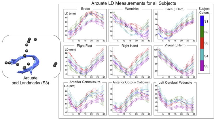
Good correspondence across normal subjects is demonstrated by measurement of landmark distances (LD) from left arcuate to nearby and distant landmarks. The plots on the right show LD measurements along the tract for all subjects. Each landmark is shown in a separate plot, with nearby landmarks in the top row. The colors indicate subject number (1 to 5). In each plot, the horizontal axis represents fiber arc length (30 points along each fiber trajectory) while the vertical axis displays LD in mm. The vertical bars represent the standard deviation of LD within each subject (across multiple fibers).

Fig. 7.

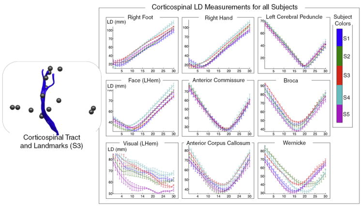
Good correspondence across normal subjects is demonstrated by measurement of landmark distances (LD) from left corticospinal tract to nearby and distant landmarks. The plots on the right show LD measurements along the tract for all subjects. Each landmark is shown in a separate plot, with nearby landmarks in the top row. The colors indicate subject number (1 to 5). In each plot, the horizontal axis represents fiber arc length (30 points along each fiber trajectory) while the vertical axis displays LD in mm. The vertical bars represent the standard deviation of LD within each subject (across multiple fibers).

The measurements were performed as follows. First to give a fixed-length LD vector for all fibers, for each subject and structure, each fiber was represented by 30 points evenly distributed along the fiber. Thirty was chosen as a reasonable number of points for these experiments because even for extremely long fibers of 150 mm there would be a point every 5 mm, on the order of two voxel lengths. Next, for each fiber, distances were measured from the 30 points to all functional and structural landmark points within the corresponding subject, and each subject’s mean and standard deviation of these distances at each point along the tract was recorded and was plotted in a unique color.

Finally to compactly represent the LD atlas across all subjects, all distances were concatenated into a single feature vector, and the mean and standard deviation of this vector across subjects were plotted (Fig. 8). In the figure, the concatenated pieces from each landmark are separated by vertical dashed lines.

Fig. 8.

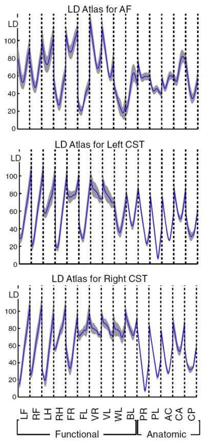
Concatenation of landmark distance information from all landmarks (previous figures) produces a single feature vector representing all LD measurements. Summarizing this information across subjects gives an LD atlas (LDA). Here, the across-subjects componentwise mean (solid blue curve) and standard deviation (gray) of the LD feature vectors are shown. The horizontal axes are labeled by anatomic and functional landmarks (for each landmark, 30 landmark distances are plotted, from points along the entire arc length of the tract). See Tables 1 and 2 for landmark acronym definitions. The vertical axes represent LD in mm. The dashed lines separate information from different landmarks (note these LDAs are not truly continuous curves, the dashed lines separate essentially unrelated datapoints that are connected by “jumps” or vertical lines due to the plotting).

Application of atlas: fiber tract prediction

We performed a leave-one-out fiber prediction experiment to test the generalization of the model to novel subjects, and to visualize the information contained in the model (Figs. 9 and 10). Each of the 5 normal subjects was chosen in turn as the test subject, and then an LD atlas was calculated for each structure (AF, left and right CST) using the mean LD for that structure across the other 4 subjects. Based on the landmark locations of the test subject, fiber predictions were then generated from the atlas using trilateration (Fig. 4) to predict each point along the fiber.

Fig. 9.

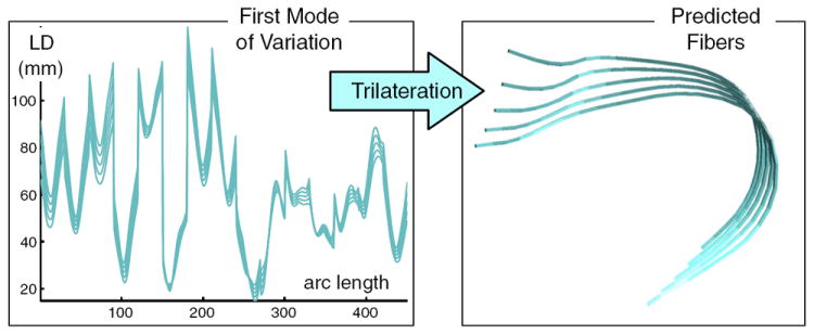
Each sample from a PCA model of the RD atlas (each curve plotted on the left) is used to predict one fiber (one trajectory on the right), via trilateration. The additional information needed to predict the fiber (landmark locations) is not displayed. This figure depicts the first mode of variation, up to ± 1 standard deviation (68% confidence interval). For simplicity, only the first mode of variation is shown, however three modes of variation were used to give the results in Fig. 10.

Fig. 10.

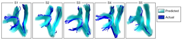
Leave-one-out prediction of tract location according to the landmark distance atlas (LDA). Each subject’s fMRI activation peaks and anatomic landmarks, plus the leave-one-out LDA from the other subjects, were used to predict the location of the AF, left CST, and right CST. The true structures for each subject are shown in dark blue, and the 68% confidence interval for the predicted trajectory is shown in transparent cyan. These results provide an alternative visualization of the data in the learned landmark distance model and they demonstrate reasonable model generalization to novel subjects.

The atlas was created using the mean LD from each of 4 subjects, and in order to take into account the cross-subject variability of this mean LD, we built a simple PCA model of the atlas. This allowed us to use the PCA modes of variation to generate multiple LD vectors for fiber prediction, and thus visualize the fiber variability deriving from our LD atlas. Specifically, we implemented a simple PCA model for each structure in the atlas, using as input the mean LD feature vector from each of the 4 subjects (Fig. 9). Samples were drawn from the model using combinations of the first three modes of variation up to±one standard deviation (sd) of each mode (where the standard deviation is the square root of the eigenvalue corresponding to the covariance matrix eigenvector that is the mode). So − 1sd, 0, and + 1sd times each mode were added to the mean LD, in combination, giving 3*3*3=27 example LD vectors spanning the space of the modes of variation. Next, for each LD vector, a fiberwas predicted using trilateration, such that 27 predicted fibers were generated for each test subject. The fibers were visualized as semi-transparent tubes (Fig. 10). These fibers can be considered to represent the 68% confidence interval of the prediction, corresponding to one standard deviation from the mean, along each mode of variation of the LD model.

The results of the fiber prediction experiment demonstrate reasonable generalization of the atlas to novel subjects, at least for the two structures (AF and CST) studied here. Other structures would require future study.

Application of atlas: fiber tract detection with displacement

We performed an experiment to assess the robustness of fiber tract detection using the LD model. The detection method takes advantage of the distinctiveness of LD feature vectors: each LD feature vector’s pattern is unique to its fiber trajectory, given the subject’s landmarks, because the fiber can be exactly re-calculated using trilateration. The LD model is invariant to rotation and translation but not to scale, thus we sought to introduce robustness to scale (such as that caused by displacement due to a mass lesion) by designing an appropriate distance measure for comparing LD feature vectors. We tested four distance measures for robustness to brain displacements.

In the following equations for the proposed distance measures, the atlas LD feature vector (blue curve in Fig. 8) for a particular tract is represented by V_LDA. This is the mean feature vector for the tract across all subjects. The LD feature vector being compared to it is V_LD. Both feature vectors are of length f×l, where f is the number of points on the fiber and l is the number of landmarks. The sums over j are over the entire length of the vectors. The standard deviation across subjects of the LDA (i.e. the across-subjects standard deviation of each subject’s mean V_LD, shown in gray in Fig. 8) at a particular point j is σ_LDA(j).

The first proposed distance measure is d_SSD, the sum of squared differences. It was chosen for testing due to its simplicity.

$$d_{\mathit{SSD}}=\sum _j{(V_{\mathit{LDA}}(j)-V_{\mathit{LD}}(j))}^2$$ (4)

The second measure is named d_Z2 since the quantity being summed is the square of the z-score, i.e. the difference from the mean over the standard deviation. It was chosen to decrease the influence of unreliable anatomical regions (those with high variability).

$$d_{Z2}=\sum _j{\left(\frac{V_{\mathit{LDA}}\left(j\right)-V_{\mathit{LD}}\left(j\right)}{{\sigma }_{\mathit{LDA}}\left(j\right)}\right)}^2$$ (5)

The third measure d_PE2 is the percent error, squared. It was designed to decrease the influence of distant landmarks that are not expected to displace with the fiber.

$$d_{\mathit{PE}2}=\sum _j{\left(\frac{V_{\mathit{LDA}}\left(j\right)-V_{\mathit{LD}}\left(j\right)}{V_{\mathit{LDA}}\left(j\right)}\right)}^2$$ (6)

The fourth proposed measure, d_CORR, is the correlation distance, and was chosen to consider the shape of the LD curves rather than the magnitude of their differences.

$$d_{\mathit{CORR}}=1-\frac{\left(V_{\mathit{LD}}-{\overline{V}}_{\mathit{LD}}\right)\text{'}\left(V_{\mathit{LDA}}-{\overline{V}}_{\mathit{LDA}}\right)}{\sqrt{\left(V_{\mathit{LD}}-{\overline{V}}_{\mathit{LD}}\right)\text{'}\left(V_{\mathit{LD}}-{\overline{V}}_{\mathit{LD}}\right)\sqrt{\left(V_{\mathit{LDA}}-{\overline{V}}_{\mathit{LDA}}\right)\text{'}\left(V_{\mathit{LDA}}-{\overline{V}}_{\mathit{LDA}}\right)}}}$$ (7)

Because the motivation for the development of the LD model was detection of displaced fiber tracts, we performed a leave-one-out experiment to assess the robustness of tract detection based on LD. Tumors can change the geometry of the brain in various ways, so we introduced two types of synthetic displacement to the data from the first control subject (Fig. 11). The first type was a synthetic spherical warp, where all fiber points and landmarks were moved outward (5 and 10 mm) from a selected point in the brain in the left hemisphere near AF and CST. This warp changed the shape of the fibers. The second type of synthetic displacement was a random translation of each entire fiber (up to 5 mm and up to 10 mm in each of x, y, and z directions). This displacement did not change the shape of the fiber, but did randomly change its relationship to the landmarks (which were left fixed). These synthetic displacements were also applied to the segmented AF and CST from subject 1, for comparison between detected and expected tracts.

Fig. 11.

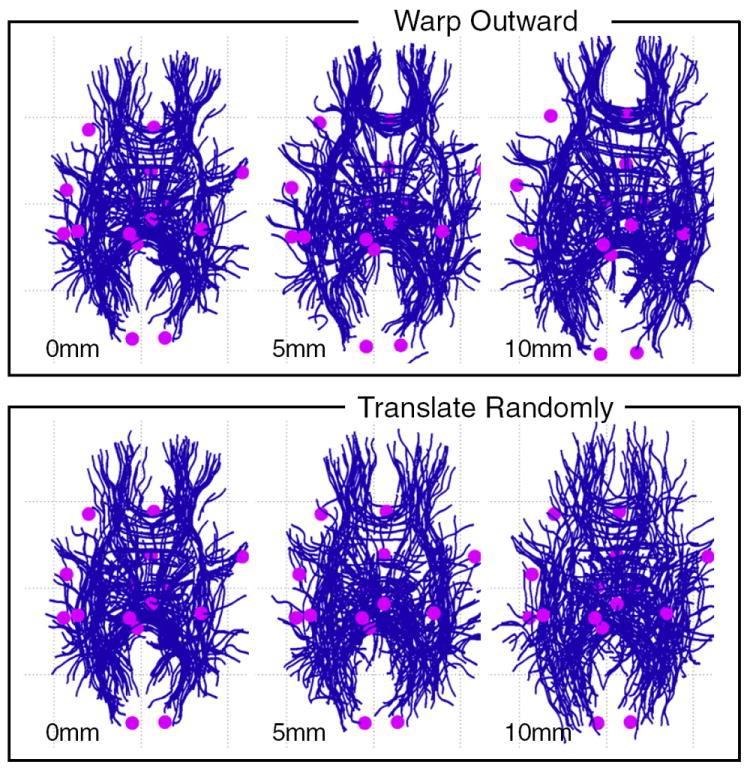
Datasets for leave-one-out testing of fiber detection with displacement. The left column (0 mm warp) shows original unwarped data from the test subject (subject 1). The two rightmost columns show synthetic data derived by applying displacements to the test subject’s data, as follows: The top row shows outward displacements of 5 mm and 10 mm applied to the tracts and landmarks (data were warped outward from an arbitrarily selected point in the left hemisphere). The bottom row shows random translations of whole fibers up to 5 mm and 10 mm along each axis (left–right, anterior–posterior, and superior–inferior). In each image, a random subset of 300 fibers is shown to reduce visual clutter.

Leave-one-out detection experiments were performed using an LD atlas from control subjects 2–5. (Note the atlas data was not synthetically warped in any way.) The atlas was applied to all datasets derived from the first subject. These datasets included the original subject 1 data with no displacement (Fig. 12), then synthetically altered subject 1 data with applied 5 mm warp, 10 mm warp (Fig. 13), up to 5 mm random translation, and up to 10 mm random translation (Fig. 14). For all experiments, the top 90 (AF) and top 30 (CST) best matching fibers and their mean LD were selected for display. (In practice this threshold could be set interactively, or a default threshold on a chosen distance measure could be learned. Here these numbers were set based on the known size of the structures in subject 1.)

Fig. 12.

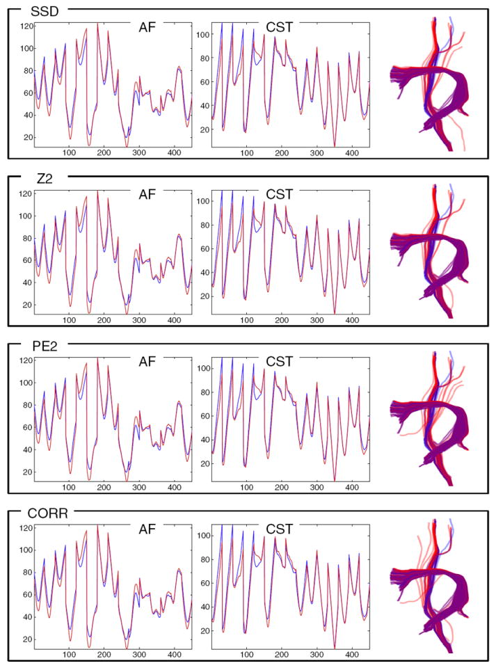
The LD model generalizes well to a test subject (subject 1) in this leave-one-out fiber detection experiment. The left two columns plot the leave-one-out AF and left CST LD atlases (blue) vs. the mean LD of detected tracts (red). The rightmost column shows the detected tracts (red) and the expected tracts (blue, from input data Fig. 2). Purple (red plus blue) indicates perfect overlap. All tested distance measures (in different rows) perform reasonably well and almost identically in this experiment (where no synthetic displacement was applied to the test subject).

Fig. 13.

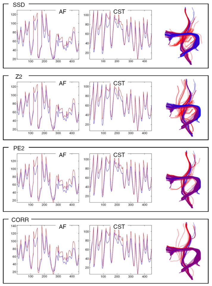
In this leave-one-out experiment the LD model generalizes well for detection of tracts warped 10 mm outward. The left two columns plot the AF and left CST LD atlases (blue) vs. the mean LD of detected tracts (red). The effect of this warp is shown in the fact that the red curve is higher in many places than the blue curve (expansion gives larger distances creating higher LD). The rightmost column shows the detected tracts (red) and the expected tracts (blue, from applying the warp to the known input tracts from Fig. 2). Purple (red plus blue) indicates perfect overlap. Comparison of detected warped tracts (right columns) indicates that performance of the PE2 and d_CORR measures is best for this kind of displacement.

Fig. 14.

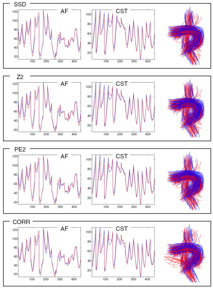
In this leave-one-out experiment the LD model generalizes well for detection of tracts randomly translated by up to 10 mm in each direction (x, y, z). The left two columns plot the AF and left CST LD atlases (blue) vs. the mean LD of detected tracts (red). The effect of this warp is not extremely visible in the mean LD curve (red), because averaging this curve over all detected fibers will tend to average out the random displacement effects. However, the expected and detected fibers (right column, in blue and red, respectively) show the effect of the warp. The top three rows’ measures perform reasonably, but the d_CORR measure (bottom row) is more sensitive to this kind of displacement and erroneously detects some fibers not part of AF or CST.

Visual inspection of detection results for each structure and displacement magnitude demonstrated that all LD distance measures perform almost identically for conditions of no displacement (Fig. 12), as well as for 5 mm displacements (these results are not shown as they were very similar to Fig. 12). For larger 10 mm displacements, the performance of the various distance measures differs. The correlation distance (d_CORR) was the most robust to the first kind of warping displacement, and the d_PE2 also gave good results (Fig. 13). The second style of random translation of up to 10 mm (Fig. 14) was handled effectively by all measures except d_CORR (which included some clearly incorrect fibers that were not part of the structures of interest). Visual inspection of results indicates that overall the d_PE2 measure (Eq. (6)) was the best able to handle the two types of displacements modeled in this experiment.

In addition to visual inspection of results, quantitative comparison of detected and expected fibers was performed by calculating the mean fiber similarity measure across all pairs of detected and expected fibers in AF and CST (Fig. 15). For fiber similarity, we employed the mean distance between pairs of closest points on two fibers, and converted to a similarity using a Gaussian kernel of sigma 30 mm (O’Donnell and Westin, 2007). Results indicate that the d_PE2 and d_CORR measures are the most successful, where the d_PE2 has better worst-case performance and d_CORR performs better in the best case. The combination of quantitative and visual inspection results from this experiment indicates that, for the synthetic displacements studied, d_PE2 is the most robust measure.

Fig. 15.

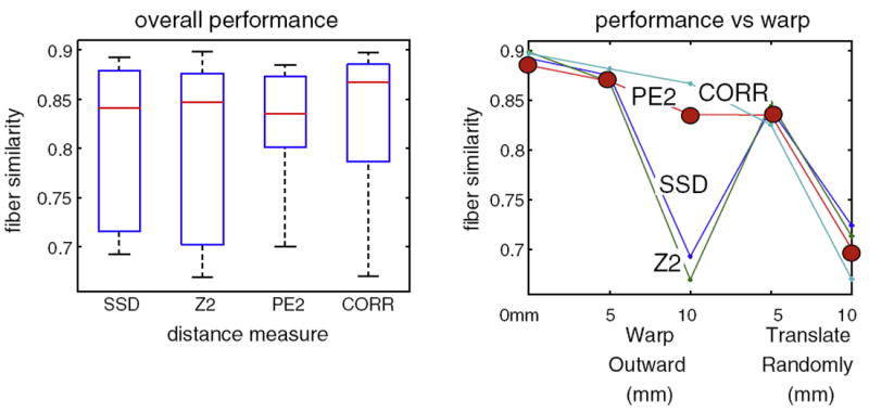
Quality of tract detection measured as mean fiber similarity between detected and expected tracts (from Figs. 12-14). On left, summary of detection performance for each LD distance measure (Application of atlas: fiber tract detection with displacement section). On right, performance of each distance measure under each warp condition: 0 mm warp (no warp), 5 and 10 mm spherical outward warp, and 5 and 10 mm random translation. Over all experiments, the most robust performance is given by the d_PE2 measure (solid circles in right graph). The d_CORR measure also performs well, but its worst-case performance is worse than the d_PE2 measure.

Application of atlas: fiber tract detection in patients

We performed an experiment to assess whether the LD of three patients was similar to the LD of the normal controls in our LD atlas. Landmark distances were measured for all fibers in the entire brain of each patient, using the fMRI activations and anatomic landmarks for that patient. The LD feature vectors of all fibers in the WM of each patient were then compared to the feature vectors of the CST and AF tracts from the LD atlas using the d_PE2 measure (Eq. (6)), where that particular measure was chosen for its success in the previous experiments. The top 30 best-matching fibers were displayed for each structure, along with their mean LD (Fig. 16). In every case, the patient had only a subset of the atlas fMRI, so the relevant subset of the LD vectors was compared. No atlas- to-patient registration was needed, as correspondence was known for the fMRI and anatomic landmarks, and the LD model is invariant to rotation and translation.

Fig. 16.

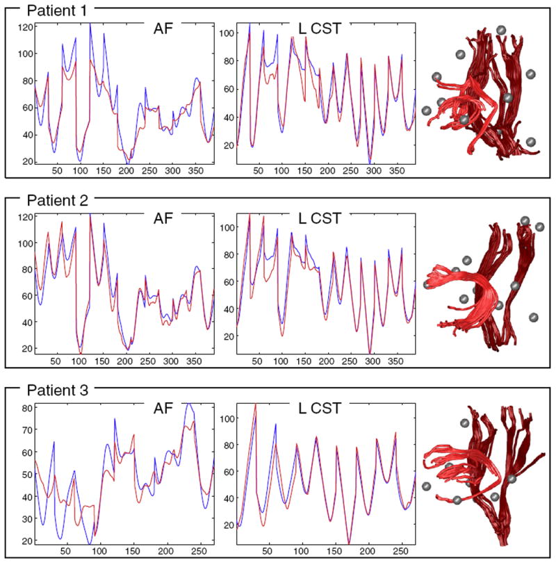
The LD model generalizes well for detection of tracts in surgical patients. The left two columns plot the AF and left CST LD atlases (blue) vs. the mean LD of detected tracts (red). The right column shows the detected structures for AF (light red) and CST (dark red). Note that missing landmark data is handled by using the corresponding subset of the atlas (all patients have fewer than 15 landmarks due to differing fMRI exams). In patients 1 and 3, the detection of the arcuate was partial due to tumor/edema near the arcuate (this can be seen in the left column’s dissimilar red and blue LD plots for AF as well as the detected tractography at right).

Results demonstrated that the mean LD from patients was similar to that of normal controls. Highly similar fibers were detected in all CSTs, and one AF. In two patients, the presence of tumor/edema prevented tracing and therefore detection of the full AF, but partial detections were seen. Fig. 17 shows the relationship of the detected tracts to the mass lesions.

Fig. 17.

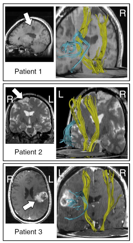
Relationship of detected AF and CST to mass lesions in patients. Left column, anatomical images showing tumor location (arrows). Right column, detected tracts, posterior oblique views. Lesions in patients 1 and 3 are located near the AF in the left hemisphere. The lesion in patient 2 is near the motor cortex, in the right hemisphere.

Discussion

Atlas individualization, or the application of standardized anatomic models to specific subjects, is a challenging problem in the presence of abnormal anatomy such as mass lesions (brain tumors). In this work we have attempted to bring together functional and structural information to create a model that may be able to generalize to patients with displaced or abnormal anatomy. We proposed a rotation and translation invariant landmark distance model that represents the spatial relationship between fiber tracts and functional/structural landmarks. By capturing this information we hope to model a fundamental anatomical structure-function relationship in the brain.

Some choices were made in designing the model that warrant discussion. We have chosen to represent fibers of varying lengths with a fixed number of points, where point spacing is determined on a perfiber basis (to evenly space points along each fiber). This allows us to measure fixed-length LD vectors for all fibers, and it simplifies the point correspondence problem across fibers and subjects. Regarding the point correspondences, we have researched several methods for representation of tracts of varying lengths. Our prior work focused on preserving distance between points, across fibers and subjects (O’Donnell et al., 2009b), however in this way endpoints of many tracts could not be analyzed due to the tracts’ differing length across subjects, despite affine registration. Work by our group and others have focused on warping tracts (i.e. Ziyan et al. (2007); Durrleman et al. (2009)) thus assuming correspondence at endpoints. However since such methods disregard other local anatomy, and local dMRI anisotropy measures determine tract termination, this assumption of endpoint correspondence is also imperfect. In the current work, we propose to analyze/represent the full length of the tract, an approach with the advantage that no data is rejected at the modeling stage. Here we do assume correspondence at tract endpoints, as well as points along the fiber. Conceptually, we believe there is no perfect approach to the point correspondence problem, due to variability across subjects in tract shape, thus we are free to explore different representations to assess their utility for various applications. For the atlasing, prediction, and detection goals of the current method, we believe that we have experimentally demonstrated that the chosen fixed-length representation performs well.

Design choices were made regarding the landmarks. We have included both functional and structural landmarks, and we chose to select landmarks manually for this initial work exploring the potential of the LD model. Theoretically, 3 or more landmarks are needed to uniquely identify a fiber. Practically, we have shown that a reduced subset of landmarks (relative to the total of 15 studied here) can be used for tract detection (Fig. 16). Future work will investigate how many/which landmarks are needed for a practical application of the proposed method.

Regarding the utility of functional versus anatomical landmarks, it is the case that the fMRI landmarks are difficult to choose reliably. In fact, their spatial variability across normal subjects was higher than that of the anatomical landmarks that we also used in the paper. This is partially due to the fact that it is not possible to fully represent an activation, with some volumetric spatial extent, by a single point. We have chosen as this point the activation peak, or maximum, a well-established practice (peak activation coordinates are often reported in fMRI studies). The motivation for including functional landmarks is that they are known to move with the fiber tract when it undergoes displacement due to a tumor (Schonberg et al., 2006). Furthermore, the spatial distribution of landmarks is important for the LD method, and the fMRI data allows us to better choose points on the cortical surface. We have shown that selection of anatomical landmarks on the cortical surface is unreliable even in expert hands (Rolls et al., 2007). A secondary motivation is to investigate whether, moving forward, such a model that relates fibers and activations can improve localization of fMRI landmarks.

We chose to employ standard single-tensor streamline tractography in this work, as tractography methods are not the focus of this paper, rather we propose methods to localize tracts of interest after tractography. However, it is clear that in the future, application of the proposed method to improved tractography would be of interest especially in structures subject to crossing fibers, such as the corticospinal tract.

Some aspects of the fiber tract prediction merit discussion. The predicted tract has the same number of points along it as the LD representation in the atlas, but these points are not constrained to have any particular distance from each other along the arc length of the predicted tract, thus the tract can be shorter or longer depending on the configuration of the landmarks in the novel subject. So if the landmarks undergo complex transformations, in some way, so does the fiber tract, however the tract is predicted according to the range of normal as far as its relation (distance) to the landmarks, without explicit measurement of the underlying transform. Currently, the clinical utility of our initial attempt at fiber prediction is unclear, and it may not be accurate, so it would only be useful if the prediction can be shown to correspond with the underlying subject data. But as a visualization of the model, and an idea to consider moving forward, we believe the fiber prediction is quite interesting. In the future it could be useful to somehow incorporate dMRI information into the prediction process.

Regarding fiber tract detection, our experiments show robustness of the model not only to rotation, translation, and scaling, but to an arbitrary spherical deformation more complex than an affine transform (Application of atlas: fiber tract detection with displacement section). It is clear that tracts in controls and patients are not related with just rotation, translation, and scaling. That is the fundamental motivation for developing a flexible model such as the LD model, where the feature vector describing the tract is somewhat insensitive to arbitrary transformations that can cause local scaling of the feature vector (Invariance to rotation and translation, and robustness to scaling or displacement section), such as displacement due to a tumor.

Overall, initial experiments presented here indicate that the LD model can generalize to novel subjects (healthy subjects and patients), and that the model is robust to displacements of the scale typically found in patients with mass lesions. These claims hold for the two structures (AF and CST) studied here, while other structures would require future study. More work is needed to rigorously test the model in retrospective patient data. Future work includes building a more complete LD atlas to represent a higher number of more finely detailed white matter structures, using data from more subjects and advanced tractography and/or diffusion models beyond the tensor.

Joint modeling of multimodality neuroimaging data is a relatively young field, and we expect that our proposed landmark distance model may have other applications. It is certainly possible to measure the model in controls, and patients with a neurological disease, and compare the two populations. It would be reasonable to apply our method if a hypothesis of abnormal structural connectivity exists.

References

- Catani M, de Schotten T. A diffusion tensor imaging tractography atlas for virtual in vivo dissections. Cortex. 2008;44(8):1105–1132. doi: 10.1016/j.cortex.2008.05.004. [DOI] [PubMed] [Google Scholar]
- Durrleman S, Fillard P, Pennec X, Trouvé A, Ayache N. A statistical model of white matter fiber bundles based on currents. In: Prince JL, Pham DL, Meyers KJ, editors. International Conference on Information Processing in Medical Imaging : Lecture Notes in Computer Science; Springer-Verlag; 2009. pp. 114–125. URL http://hal.inria.fr/inria-00502721/en/ [DOI] [PubMed] [Google Scholar]
- Fischl B, Salat D, Busa E, Albert M, Dieterich M, Haselgrove C, van der Kouwe A, Killiany R, Kennedy D, Klaveness S, et al. Whole brain segmentation: automated labeling of neuroanatomical structures in the human brain. Neuron. 2002;33(3):341–355. doi: 10.1016/s0896-6273(02)00569-x. [DOI] [PubMed] [Google Scholar]
- Glasser MF, Rilling JK. DTI tractography of the human brain’s language pathways. Cereb Cortex. 2008;18(11):2471–2482. doi: 10.1093/cercor/bhn011. [DOI] [PubMed] [Google Scholar]
- Gong G, He Y, Concha L, Lebel C, Gross DW, Evans AC, Beaulieu C. Mapping anatomical connectivity patterns of human cerebral cortex using in vivo diffusion tensor imaging tractography. Cereb Cortex. 2009;19(3):524–536. doi: 10.1093/cercor/bhn102. [DOI] [PMC free article] [PubMed] [Google Scholar]
- Goodlett C, Davis B, Jean R, Gilmore J, Gerig G. Improved correspondence for DTI population studies via unbiased atlas building. Lect Notes Comput Sci. 2006;4191:260. doi: 10.1007/11866763_32. [DOI] [PubMed] [Google Scholar]
- Greicius MD, Supekar K, Menon V, Dougherty RF. Resting-state functional connectivity reflects structural connectivity in the default mode network. Cereb Cortex. 2009;19(1):72–78. doi: 10.1093/cercor/bhn059. [DOI] [PMC free article] [PubMed] [Google Scholar]
- Håberg A, Kvistad K, Unsgård G, Haraldseth O. Preoperative blood oxygen level-dependent functional magnetic resonance imaging in patients with primary brain tumors: clinical application and outcome. Neurosurgery. 2004;54(4):902–915. doi: 10.1227/01.neu.0000114510.05922.f8. [DOI] [PubMed] [Google Scholar]
- Hagler D, Jr, Ahmadi M, Kuperman J, Holland D, McDonald C, Halgren E, Dale A. Automated white-matter tractography using a probabilistic diffusion tensor atlas: application to temporal lobe epilepsy. Hum Brain Mapp. 2009;30(5):1535. doi: 10.1002/hbm.20619. [DOI] [PMC free article] [PubMed] [Google Scholar]
- Holodny AI, Watts R, Korneinko VN, Pronin IN, Zhukovskiy ME, Gor DM, Ulug A. Diffusion tensor tractography of the motor white matter tracts in man: Current controversies and future directions. Ann N Y Acad Sci. 2005;1064:88–97. doi: 10.1196/annals.1340.016. [DOI] [PubMed] [Google Scholar]
- Hua K, Oishi K, Zhang J, Wakana S, Yoshioka T, Zhang W, Akhter KD, Li X, Huang H, Jiang H, van Zijl P, Mori S. Mapping of functional areas in the human cortex based on connectivity through association fibers. Cereb Cortex (bhn215) 2008a doi: 10.1093/cercor/bhn215. [DOI] [PMC free article] [PubMed] [Google Scholar]
- Hua K, Zhang J, Wakana S, Jiang H, Li X, Reich D, Calabresi P, Pekar J, van Zijl P, Mori S. Tract probability maps in stereotaxic spaces: analyses of white matter anatomy and tract-specific quantification. Neuroimage. 2008b;39(1):336–347. doi: 10.1016/j.neuroimage.2007.07.053. [DOI] [PMC free article] [PubMed] [Google Scholar]
- Kamada K, Sawamura Y, Takeuchi F, Kawaguchi H, Kuriki S, Todo T, Morita A, Masutani Y, Aoki S, Kirino T. Functional identification of the primary motor area by corticospinal tractography. Neurosurgery. 2005;56:98–109. doi: 10.1227/01.neu.0000144311.88383.ef. [DOI] [PubMed] [Google Scholar]
- Lele S, Richtsmeier J. Euclidean distance matrix analysis: a coordinate-free approach for comparing biological shapes using landmark data. Am J Phys Anthropol. 1991;86(3):415–427. doi: 10.1002/ajpa.1330860307. [DOI] [PubMed] [Google Scholar]
- Maddah M, Grimson W, Warfield S, Wells W. A unified framework for clustering and quantitative analysis ofwhite matter fiber tracts. Med Image Anal. 2008;12(2):191–202. doi: 10.1016/j.media.2007.10.003. [DOI] [PMC free article] [PubMed] [Google Scholar]
- Mori S, Wakana S, Nagae-Poetscher LM, van Zijl PC. MRI Atlas of Human White Matter. Elsevier; 2005. [DOI] [PubMed] [Google Scholar]
- Mori S, Oishi K, Jiang H, Jiang L, Li X, Akhter K, Hua K, Faria AV, Mahmood A, Woods R, Toga AW, Pike GB, Neto PR, Evans A, Zhang J, Huang H, Miller MI, van Zijl P, Mazziotta J. Stereotaxic white matter atlas based on diffusion tensor imaging in an ICBM template. Neuroimage. 2008;40(2):570–582. doi: 10.1016/j.neuroimage.2007.12.035. [DOI] [PMC free article] [PubMed] [Google Scholar]
- O’Donnell L, Westin C-F. Automatic tractography segmentation using a high-dimensional white matter atlas. IEEE Trans Med Imaging. 2007;26(11):1562–1575. doi: 10.1109/TMI.2007.906785. [DOI] [PubMed] [Google Scholar]
- O’Donnell LJ, Rigolo LE, Norton I, Westin C-F, Golby AJ. Defining spatial relationships between fmri and dti fiber tracts. MICCAI Workshop on Diffusion Modeling and the Fibre Cup 2009a [Google Scholar]
- O’Donnell LJ, Westin C-F, Golby AJ. Tract-based morphometry for white matter group analysis. Neuroimage. 2009b;45(3):832–844. doi: 10.1016/j.neuroimage.2008.12.023. [DOI] [PMC free article] [PubMed] [Google Scholar]
- O’Shea JP, Whalen S, Branco DM, Petrovich NM, Knierim KE, Golby AJ. Integrated image- and function-guided surgery in eloquent cortex: a technique report. Int J Med Robot. 2006;2(1):75–83. doi: 10.1002/rcs.82. [DOI] [PubMed] [Google Scholar]
- Pohl K, Fisher J, Grimson W, Kikinis R, Wells W. A Bayesian model for joint segmentation and registration. Neuroimage. 2006;31(1):228–239. doi: 10.1016/j.neuroimage.2005.11.044. [DOI] [PubMed] [Google Scholar]
- Rolls HK, Yoo S-S, Zou KH, Golby AJ, Panych LP. Rater-dependent accuracy in predicting the spatial location of functional centers on anatomical MR images. Clin Neurol Neurosurg. 2007;109(3):225–235. doi: 10.1016/j.clineuro.2006.08.005. [DOI] [PMC free article] [PubMed] [Google Scholar]
- Schonberg T, Pianka P, Hendler T, Pasternak O, Assaf Y. Characterization of displaced white matter by brain tumors using combined DTI and fMRI. Neuroimage. 2006;30(4):1100–1111. doi: 10.1016/j.neuroimage.2005.11.015. [DOI] [PubMed] [Google Scholar]
- Skudlarski P, Jagannathan K, Calhoun VD, Hampson M, Skudlarska BA, Pearlson G. Measuring brain connectivity: diffusion tensor imaging validates resting state temporal correlations. Neuroimage. 2008;43(3):554–561. doi: 10.1016/j.neuroimage.2008.07.063. [DOI] [PMC free article] [PubMed] [Google Scholar]
- Tucholka A, Thirion B, Pinel P, Poline J-B, Mangin J-F. Triangulating cortical functional networks with anatomical landmarks. ISBI. 2008:612–615. [Google Scholar]
- Venkataraman A, Rathi Y, Kubicki M, Westin C-F, Golland P. Joint generative model for fmri/dwi and its application to population studies. Med Image Comput Comput Assis t Interv. 2010;13(Pt. 1):191–199. doi: 10.1007/978-3-642-15705-9_24. [DOI] [PMC free article] [PubMed] [Google Scholar]
- Worsley K, Friston K. Analysis of fMRI time-series revisited-again. Neuroimage. 1995;2(3):173–181. doi: 10.1006/nimg.1995.1023. [DOI] [PubMed] [Google Scholar]
- Yushkevich PA, Zhang H, Simon TJ, Gee JC. Structure-specific statistical mapping of white matter tracts. Neuroimage. 2008;41(2):448–461. doi: 10.1016/j.neuroimage.2008.01.013. [DOI] [PMC free article] [PubMed] [Google Scholar]
- Zhang W, Olivi A, Hertig S, van Zijl P, Mori S. Automated fiber tracking of human brain white matter using diffusion tensor imaging. Neuroimage. 2008;42(2):771–777. doi: 10.1016/j.neuroimage.2008.04.241. [DOI] [PMC free article] [PubMed] [Google Scholar]
- Ziyan U, Sabuncu MR, O’Donnell LJ, Westin C-F. Nonlinear registration of diffusion MR images based on fiber bundles. MICCAI. 2007:351–358. doi: 10.1007/978-3-540-75757-3_43. [DOI] [PubMed] [Google Scholar]