Functional Roles for Synaptic-Depression within a Model of the Fly Antennal Lobe

Abstract

Several experiments indicate that there exists substantial synaptic-depression at the synapses between olfactory receptor neurons (ORNs) and neurons within the drosophila antenna lobe (AL). This synaptic-depression may be partly caused by vesicle-depletion, and partly caused by presynaptic-inhibition due to the activity of inhibitory local neurons within the AL. While it has been proposed that this synaptic-depression contributes to the nonlinear relationship between ORN and projection neuron (PN) firing-rates, the precise functional role of synaptic-depression at the ORN synapses is not yet fully understood. In this paper we propose two hypotheses linking the information-coding properties of the fly AL with the network mechanisms responsible for ORNAL synaptic-depression. Our first hypothesis is related to variance coding of ORN firing-rate information — once stimulation to the ORNs is sufficiently high to saturate glomerular responses, further stimulation of the ORNs increases the regularity of PN spiking activity while maintaining PN firing-rates. The second hypothesis proposes a tradeoff between spike-time reliability and coding-capacity governed by the relative contribution of vesicle-depletion and presynaptic-inhibition to ORNAL synaptic-depression. Synaptic-depression caused primarily by vesicle-depletion will give rise to a very reliable system, whereas an equivalent amount of synaptic-depression caused primarily by presynaptic-inhibition will give rise to a less reliable system that is more sensitive to small shifts in odor stimulation. These two hypotheses are substantiated by several small analyzable toy models of the fly AL, as well as a more physiologically realistic large-scale computational model of the fly AL involving glomerular channels.

Author Summary

Understanding the intricacies of sensory processing is a major scientific challenge. In this paper we examine the early stages of the olfactory system of the fruit-fly. Many experiments have revealed a great deal regarding the architecture of this system, including the types of neurons within it, as well as the connections those neurons make amongst one another. In this paper we examine the potential dynamics produced by this neuronal network. Specifically, we construct a computational model of this early olfactory system and study the effects of synaptic-depression within this system. We find that the dynamics and coding properties of this system depend strongly on the strength, and sources of, synaptic-depression. This work has ramifications for understanding the coding properties of other insect olfactory systems, and perhaps even other sensory modalities in other animals.

Introduction

The early stages of the drosophila olfactory system include a primary sensory structure called the antenna lobe (AL). The AL receives input from olfactory sensory neurons (ORNs) at the sensory periphery, and is organized into glomerular clusters, with each cluster corresponding to a specific olfactory receptor class [1]–[5]. Each glomerulus within the AL contains dendrites of local neurons (LNs) whose projections are limited to the AL, as well as projection neurons (PNs) whose axons extend beyond the AL deeper into the fly brain [6]. The PNs are excitatory, whereas there is evidence that both excitatory local neurons (LNEs) and inhibitory local neurons (LNIs) exist [7]–[9]. The LNs associated with each glomerulus have local projections, which connect to that glomerulus, as well as lateral projections which connect to other glomeruli [10].

Various experiments indicate that there exists substantial synaptic-depression at the synapses between olfactory receptor neurons (ORNs) and neurons within the drosophila antenna lobe (AL); by ‘synaptic-depression’, we refer to any mechanism which gives rise to short-term depression of the ORN-induced EPSCs within the AL following an increase in ORN activity. While it has been proposed that this synaptic-depression contributes to the nonlinear relationship between ORN and PN firing-rates, the precise functional role of synaptic-depression at the ORN synapses is not yet fully understood. To investigate the relationship between synaptic-depression and the coding properties of the fly AL, we created and analyzed the dynamics of several models of the fly AL. We have been able to distill two hypotheses linking the information-coding properties of the fly AL with the network mechanisms responsible for ORNAL synaptic-depression.

Our first hypothesis is related to the variance coding of ORN firing-rate information — once stimulation to the ORNs is sufficiently high to saturate PN responses within any particular glomerular channel, further stimulation of the ORNs can reduce the amount of fluctuation of the ORNPN input within that channel, thus increasing the regularity of PN spiking activity while maintaining PN firing-rates. Thus, given two different stimuli which saturate the responses of a given glomerulus, it may still be possible to distinguish between these two stimuli solely by using this saturated glomerulus' activity. In order to distinguish these saturated responses, a readout mechanism must be sensitive to higher-order statistics (such as variance) in the saturated glomerulus' activity.

Our second hypothesis proposes a tradeoff between trial-to-trial reliability and sensitivity governed by the mechanisms responsible for ORNAL synaptic-depression. Within the fly, synaptic-depression may be partly caused by vesicle-depletion, and partly caused by presynaptic-inhibition due to the activity of inhibitory local neurons within the AL [11], [12]. Our second hypothesis is that synaptic-depression caused primarily by vesicle-depletion will give rise to a very reliable system, whereas an equivalent amount of synaptic-depression caused primarily by presynaptic-inhibition will give rise to a less reliable system that is more sensitive to small shifts in odor stimulation. Using this second hypothesis, one can further postulate that a balance of vesicle-depletion and presynaptic-inhibition within the AL is required in order to optimize the discriminability of the network over short observation-times.

Results

The relationship between the architecture of the fly AL and its odor-coding properties largely remain a mystery. Specifically, the precise functional role of synaptic-depression at the ORN synapses is still unclear. In order to investigate the possible function associated with these network mechanisms, we have designed and built a scaled down computational network model of the fly AL. By analyzing the dynamics of this model we have been able to distill two hypotheses linking the information-coding properties of the fly AL with the network mechanisms responsible for ORNAL synaptic-depression. We will discuss these hypotheses later in the sections below, after first introducing a few pertinent details regarding our computational model.

Sketch of computational network model

In brief, our computational network model incorporates glomerular channels, each with PNs, LNEs, LNIs and ORNs, in rough accordance with the experimentally observed ratio of ORNs to PNs and LNs [13]. As the real fly AL has glomerular compartments, each of roughly this size [10], this model is the size of the full AL. Each neuron in this network model is modeled using Hodgkin-Huxley-type equations. The synaptic currents in this network allow neurons to affect other neurons in the same glomerulus, as well as neurons in other glomeruli. The input to this network takes the form of noisy stimulus current to the ORNs, with different ‘odors’ corresponding to different levels of stimulus current to different ORN input channels. Importantly, the model is built to accommodate synaptic-depression of the ORN synapses, allowing for both the mechanisms of presynaptic-inhibition as well as vesicle-depletion. An illustration of the network's connectivity, as well as an abridged list of network parameters, is given in Fig. 1. We have built this network to respect physiological constraints, and we have tuned this model using several experiments as benchmarks. Here we provide a brief summary of these results. A more detailed description of the model as well as the details regarding the benchmarking are contained in the Methods section.

Figure 1. A schematic of the large-scale network model.

[Left]: The network consists of 5 glomerular channels, each incorporating 60 olfactory receptor neurons (ORNs in green) which stimulate a ‘glomerulus’ consisting of 6 projection neurons (PNs in red), 6 excitatory local neurons (LNEs in magenta) and 6 inhibitory local neurons (LNIs in blue). The PNs, LNEs and LNIs are connected to one another randomly within each glomerulus, and the LNEs and LNIs also affect the neurons in other glomeruli. The LNIs affect the ORNAL synapses via presynaptic-inhibition. [Right]: The non-negligible connection strengths are listed on top, with the slow-inhibitory connection strengths listed separately from the fast-inhibition strengths. The relevant connection probabilities are listed on the bottom. The parameter refers to , which characterizes the overall strength of presynaptic-inhibition. See Methods for full details.

Our goal while benchmarking this model was to ensure that our model produced reasonable statistical features of AL activity during the following odor onset. The reason we focused on matching the statistics of this transient period is that evidence indicates that this period is likely critical for many basic olfactory discrimination and classification tasks [14], [15]. One of the simplifications we have made in our model is that the input to the ORNs following odor onset is assumed to be a Poisson process with a time-varying rate that is roughly stereotyped across ORN classes (see Methods). While natural odor stimuli are likely temporally complex [16] and even static stimuli generate odor-specific temporal fluctuations at the level of the fly ORNs after several hundred ms [17], the dynamics of the ORN responses during the first following odor onset seems to be relatively stereotypical, involving either a sharp increase in activity or, more rarely, an inhibitory phase [18], [19]. Thus, the idealized input to the ORNs we employ in our model is intended to capture these simple features of ORN activity which drive the AL during the first following odor onset.

The experimental phenomena we used to benchmark our model ultimately provided three constraints on the connectivity of our model network. First, the convergence ratio of ORNs to PNs must be high, otherwise the PNs do not receive sufficient convergent input to fire quickly after odor onset. Second, the synaptic-depression at the ORN synapses must be sufficient to ensure that PN firing-rates peak earlier than ORN firing-rates (in response to odor stimulus), and that ORNPN input is strong and relatively stable during the first after odor stimulus onset. Finally, the inter-AL connectivity (governed by the LNLN, PNPN, PNLN, and LNPN connection matrix) must be sufficiently strong to create PNs which are more broadly responsive than their ORN inputs, yet sufficiently sparse to place the network in a dynamic regime which does not develop spontaneous oscillations (which are not observed experimentally during the initial transient following odor onset – [17]).

In addition, to further understand the network mechanisms underlying the two proposed hypotheses, we have designed simpler neuronal network models which distill the relevant phenomena, while allowing for a more comprehensive analysis. The analytical tools we use include the analysis of return-maps for simple network models, as well as the analysis of population-dynamics equations for more complicated network models (see the sections to follow for more details).

Hypothesis 1: a monotonically decreasing map between ORN activity and PN input variance

As evidenced in [20], [21], the relationship between ORN firing-rate () and PN firing-rate () for a given glomerulus is often nonlinear, with the PN firing-rate saturating rather quickly as a function of ORN firing-rate. One consequence of this nonlinearity is that, for low , the gain in is high — as varies from 0–50 Hz, can vary from 0–150 Hz or more. Another consequence of the nonlinear relationship is that, for high , the gain in is low — as varies from 100–200 Hz, may remain almost constant. Many have noted that the region of high gain allows for ‘odor separation’ — namely, odors which give rise to similar profiles for a given glomerulus may in turn produce very different profiles within that glomerulus [20]. However, this ‘odor separation’ only works when the odors in question generate which are sufficiently low as to lie in the region of high gain. It is tempting to conclude that if two odors generate which are sufficiently high (such that the induced lie in the region of low gain), then the generated by these odors would be similar, and the odors would not be ‘separated’.

The first hypothesis we propose is that, even if two odors generate which correspond to similar , the dynamics of the glomerulus may still serve to separate these odors. However, in this case the odor separation takes place not in terms of PN firing-rates (as, indeed, the generated by these two odors may be very similar or identical), but rather in terms of higher-order statistics of PN activity. In other words, even though the set of PN firing-rates produced at the plateau of the relationship are similar, we hypothesize that there is in fact a systematic difference in the PN dynamics underlying these similar PN firing-rates.

To be more specific, we claim that for values of along the plateau of the relationship, as increases (and stays roughly the same), the synaptic-depression at the ORN synapses continues to increase. One consequence of this increase in synaptic-depression is that, as increases along the plateau of , the number of ORN firing-events increases, but the effect of each ORN firing-event on postsynaptic PNs decreases. Thus, the postsynaptic conductance induced within any PN by the ORNs (i.e., the ORN input to the PN) maintains roughly the same mean, but decreases in variance. When discussing a reduction in the variance of ORN input, we refer specifically to a reduction in the variance across short time-windows of the PN excitatory-conductance due to ORN activity.

If the is not very high, then each ORN generates relatively few spikes, each resulting in a large EPSC in the postsynaptic PN. Thus, the ORN input to the PNs will have large fluctuations (i.e., the PNs will be ‘fluctuation-driven’). On the other hand, if is very high, then each ORN generates very many spikes, each resulting in a small EPSC within the postsynaptic PN. In this case the PN conductance due to the ORNs will be nearly constant (and the PNs will be ‘mean-driven’). We further hypothesize that, as increases along the plateau of , the decrease in variance of ORN input to the PNs will correspond to a decrease in the variance of PN spiking activity. Because (i) the ORN activity is not deterministic, but rather driven by many independent stochastic molecular binding events [18], and (ii) many ORNs are presynaptic to each PN, the accumulation of ORN firing-events observed by any given PN during any trial of odor presentation is well-approximated by a Poisson process with time-varying rate. Thus, a decrease in the ORN input variance across short time-windows will be associated with a decrease in the ORN input variance across multiple trials (for the same time-window). Thus, one would expect the variance in PN spiking activity mentioned above to decrease both across short time-windows and across multiple trials (for the same time-window). This reduction in variance of PN spiking activity is equivalent to an increase in the regularity of PN spiking activity, which is equivalent to a reduction in the variance of the inter-spike-interval distribution associated with a PN within the given glomerulus.

Thus, in summary, our first hypothesis is that the dynamics of a glomerulus can serve to separate ORN inputs in two ways. Not only can similar ORN inputs within the high-gain region of be mapped to significantly different PN firing-rates (see [20]), but ORN inputs within the low-gain region of can give rise to PN activity with differing degrees of regularity, even when the PN firing-rates associated with those ORN inputs are not significantly different. This hypothesis may have significance for odor discrimination, as the variance in PN activity may encode features of the odor even in situations where the ORN input is sufficiently high that PN firing-rates have saturated (see Discussion).

A simple cartoon of variance coding

As a simple cartoon which illustrates this hypothesis, we have simulated a single conductance-based integrate-and-fire PN, driven by a set of ORNs, each endowed with a simple model of synaptic-depression. This simple model exhibits the following dynamical features: (i) the relationship exhibits high gain and saturation, and (ii) for different values of on the plateau of the relationship, the variance in PN activity decreases as increases, even though remains roughly constant.

Within this simple model, we describe each ORN as a Poisson process with fixed rate ( ). The coupling strength between the ORNs and the PN is modulated by a term (), which is intended to model vesicle-depletion at the ORN synapses. As each ORN fires, this term will give rise to synaptic-depression between the ORNs and the PN. If , the synapses between the ORNs and the PN are exhausted. If , the synapses between the ORNs and the PN are completely refreshed. The model details are given in a section entitled “An idealized model used to illustrate variance coding” in Methods.

With this simple model, it can be seen that the PN firing-rate is a nonlinear function of the ORN firing-rate , and that saturates (plateaus) at values of (See Fig. 2A). The time-averaged mean total excitatory conductance of the PN enjoys a similar nonlinear relationship (Fig. 2B). Notably, for values of , the time-averaged mean vesicle-depletion parameter increases as a function of , and the standard deviation in the total PN conductance decreases as a function of (Fig. 2C and Fig. 2D). This decrease in standard deviation is associated with a decrease in coefficient-of-variation for the total PN conductance. Qualitatively speaking, the PN is more ‘mean driven’ when , and the PN is more ‘fluctuation driven’ when , even though the firing-rate of the PN is similar in both cases (Fig. 2E and Fig. 2F). This can be quantified by measuring, for example, the autocorrelation of the PN. In the case , the PN autocorrelation shows several significant peaks, the first of which is at , indicating periodic-firing at (Fig. 2E). In the case , the PN autocorrelation does not indicate a strong periodicity to the PN firing-patterns (Fig. 2E).

Figure 2. A simple illustration of variance coding.

Here we presume the simple model described in the section entitled “An idealized model used to illustrate variance coding”. [A] There is a nonlinear relationship between the ORN firing-rate and the PN firing-rate. [B] There is also a nonlinear relationship between the ORN firing-rate and the time-averaged conductance of the PN. [C] As the ORN firing-rate increases, the time-averaged vesicle-depletion parameter increases and saturates. [D] Since the average vesicle-depletion parameter increases as the ORN firing-rate increases, the variance in the PN conductance is a decreasing function of ORN firing-rate, for sufficiently high ORN firing-rates. Two different points along this curve are indicated, corresponding to two different PN dynamical regimes with similar PN firing-rates. The ‘’ and ‘’ symbols indicate, respectively, an irregularly firing-regime and a regularly firing-regime. [E] As a result of the fact that the PN conductance has a low variance when the ORN firing-rates are high, the PN activity is very regular when the ORN firing-rate is high. In contrast, the PN activity is less regular when the ORN firing-rate is not as high. This is reflected in the normalized PN autocorrelation, which shows several significant peaks when the variance in the PN conductance is low (‘’-regime, left). In contrast, when the variance in the PN conductance is high the autocorrelation does not show significant peaks (‘’-regime, right). [F] The regularity in the PN spiking activity is seen in PN voltage trace, as shown for the ‘’-regime (top) and ‘’-regime (bottom). [G] The variance in the PN conductance is seen in PN conductance trace, as shown for the ‘’-regime (top) and ‘’-regime (bottom). [H] In this panel we show the voltage-trace of a putative Kenyon cell, a conductance-based integrate-and-fire-neuron, driven by either the PN from the -regime (top) or the PN from the -regime (bottom). Thick vertical lines indicate firing-events for this putative KC. When driven by the regular activity of the -PN, the KC mainains an elevated subthreshold voltage, but does not fire often. On the other hand, when driven by the irregular activity of the -PN, the KC does not maintain an elevated subthreshold voltage but fires after each burst in -PN-activity. This provides a simple illustration of one possible way in a variance-code could be ‘read-out’ by downstream neurons.

The simple cartoon described above only considers synaptic-depression resulting from vesicle-depletion. The real AL displays evidence of presynaptic-inhibition as well. Nevertheless, the same general principle still holds regardless of the source of synaptic-depression at the ORN synapses, as long as the PNs become more mean driven as ORN firing-rates increase. In fact, it is possible to show analytically that similar results hold across a wide range of parameters for an idealized system similar to this one (see the section entitled “A simple analyzable cartoon of variance coding” in Methods).

If this picture is accurate in the real AL, then the PN dynamics within any given glomerulus in the AL will change as a function of ORN input to that glomerulus, even when the mean PN firing-rates have saturated for that glomerulus. These dynamical changes will only be observable through measurements of statistics that are ‘higher-order’ than mean firing-rate. We note that synaptic-depression of the ORN synapses is not the only mechanism via which the PNs may become more mean-driven as ORN firing-rates increase — other mechanisms, such as spike-frequency adaptation, could also contribute to this effect. As long as the postsynaptic influence of each ORN spike decreases as increases, the PN activity will become more mean-driven as increases. As the PN activity becomes more mean-driven, we expect the firing-sequences produced by that PN to become more regular [22].

An illustration of variance coding within a large-scale model

We also observe this phenomenon within our large-scale model (described in Methods), which contains both presynaptic-inhibition and vesicle-depletion. To illustrate this phenomenon at work, we created a panel of 16 odors, all of which saturated the PN firing-rates (i.e., produced average PN firing-rates at the ‘plateau’ of the curve for the model). We presented each of these odors to the model network times.

For each of the trials of each stimulus we measured the -component vector of PN firing-counts collected over the following odor onset. Each component of this vector represents the number of spikes fired by one of the PNs during this time. We then used this vector to perform each possible -way and -way stimulus discrimination task (see the section entitled “Odor Discrimination” in the Methods). Each of these -way and -way discrimination tasks results in a discriminability rate (i.e., the fraction of correctly categorized trials – note that chance performance for a -way task is , and chance performance for a -way task is ).

We construct a histogram of the discriminability rates for the -way discrimination tasks, and as expected (see Fig. 3A), the typical discriminability rate for the system is not particularly high (recall that each odor saturated the PN firing-rates). Similarly, the -way discrimination tasks performed using PN firing-rate vectors also do not yield high discriminability rates (Fig. 3B). However, if instead of merely using PN firing-rate information we also use information regarding PN-PN correlations within the system, then the typical discriminability rates for the -way and -way tasks increase (see Fig. 3C,D). To produce the discriminability rates shown in Fig. 3C,D, we measured not only the -component vector of PN firing-counts for each odor trial, but also the -component vector of PN-PN correlations (with correlation time ). As expected, these higher-order statistics contain enough information to discriminate odors significantly more reliably than mere firing-rates.

Figure 3. A manifestation of variance coding within the large-scale model.

The large scale model (described in Methods) exhibits a phenomenon similar to the variance coding shown in Fig. 2. We constructed a panel of 16 odors, all of which only directly stimulated the same glomeruli (although to differing degrees). Moreover, we chose every odor within this panel such that the ORN firing-rates of the directly stimulated glomeruli were sufficient to saturate the firing-rates of the associated PNs (i.e., the directly stimulated ORN firing-rates were 12 Hz, see Fig. 10). Given this panel of odors, we presented each odor multiple times, and used the collection of -component PN firing-rate vectors (measured over the period immediately following odor onset) to perform a variety of odor discrimination tasks (see Results for details). [A] The histogram of discriminability rates associated with -way discrimination tasks when only firing-rate data is used. Note that is chance level for these tasks (chance level is also shown in panels B,C,D). [B] The histogram of discriminability rates associated with the -way discrimination tasks when only firing-rate data is used (note that is chance level for these tasks). [C] The histogram of discriminability rates associated with -way discrimination tasks when firing-rate data and -point correlations (correlation time ) are used. [D] The histogram of discriminability rates associated with -way discrimination tasks when firing-rate data and -point correlations (correlation time ) are used. Note that the typical discriminability rate is higher when correlations are used. [E] Here we plot the difference in mean discriminability for the -way discrimination task between the cases (i) when firing-rate data and -point correlations are used, and (ii) only firing-rate data is used. We plot this difference as a function of the parameters and used in our large-scale model. The vesicle-depletion parameter ranges from to across the vertical axis, and the presynaptic-inhibition parameter ranges from to across the horizontal axis. The data shown in panels A–D is taken from the simulation indicated by the dashed square. Note that, as the total amount of synaptic-depression decreases, the discriminability computed using only firing-rates is closer to the discriminability computed using both firing-rates and -point correlations. [F] Similar to panel-E, except for the -way discrimination task, rather than the -way discrimination task.

The difference between the performance of these low-order and high-order readouts is more noticeable when the synaptic-depression in the system is strong. Conversely, in a network with no vesicle-depletion and reduced presynaptic-inhibition, the low- and high-order readouts yield more similar discriminability-rates (see Fig. 3E,F). Thus, the presence of strong synaptic-depression within our system is one factor which allows the network's dynamics to encode input-specific information within the PN-PN correlations.

For the example shown in Fig. 3, the difference between the typical 2-way discriminability rates observed when using high-order versus low-order readouts is maximized when the synaptic-depression is strongest; the effect of variance coding is seen quite clearly. However, for the 3-way discriminability rates, the difference between the high- and low-order readouts is greatest when the presynaptic-inhibition is not too strong. A natural question is: why does the performance for the 3-way discrimination task not parallel that for the 2-way task? Why is the difference in performance between high- and low-order readouts not maximized when both presynaptic-inhibition and vesicle-depletion are at their strongest?

This effect arises in part because the 3-way task is quite difficult and the observation time over which the task is carried out is rather short — in this case. As we will argue below, one consequence of strong presynaptic-inhibition is that the network's ability to perform fine discrimination will be compromised when is small. In order to perform very well on fine discrimination tasks when is small, the network should have only moderate amounts of presynaptic-inhibition (consistent with Fig. 3F).

Hypothesis 2: a tradeoff between reliability and sensitivity

It has been hypothesized that one functional role for the AL is to separate similar odors and that the nonlinear gain curve is instrumental in this process. As shown in [11], the nonlinearity of is influenced strongly by substantial synaptic-depression at the ORN synapses. Thus, it is reasonable to conclude that one functional role of synaptic-depression at the ORN synapses is to enhance the odor separation capabilities of the AL.

Within the fly AL there are multiple sources of synaptic-depression at the ORN synapses. Two major mechanisms which contribute to this synaptic-depression are vesicle-depletion and presynaptic-inhibition. While either one of these mechanisms could, in principle, be the major contributing factor to the synaptic-depression observed within the fly AL, it seems as though both of these mechanisms play a substantial role in producing synaptic-depression [11], [12]. Thus, one is faced with the following natural question: What purpose do these two distinct mechanisms serve within the fly AL? How would the odor-coding properties of the fly AL change if, say, only one of these mechanisms were responsible for the observed levels of synaptic-depression at the ORN synapses? Is there some functional advantage gained by having both of these mechanisms at play?

In what follows we introduce a hypothesis which links the underlying nature of synaptic-depression at the ORN synapses to information-coding properties of the AL, such as reliability, sensitivity and discriminability. First we will define these terms, and then we will explain our hypothesis in more detail throughout the rest of this section.

sources of noise: There are two sources of ‘noise’ in our network which influence the reliability (or unreliability) of the AL's activity across trials. The first is the initial condition of the system (i.e., the state of the system at odor onset). Different initial conditions will give rise to different dynamic trajectories. The second source of noise is the odor-driven Poisson input to the ORNs in the model. Different trials will give rise to different sequences of ORN spikes.

reliability: We define the reliability of the AL as the inverse of the coefficient-of-variation in spike-counts of AL neurons, as measured across trials over a given stimulus-driven time-window. Reliability is high if the spike-counts of the AL neurons are similar from trial-to-trial. Reliability is low if the spike-counts vary significantly from trial to trial. In our analysis we will consider a family of networks with the same mean firing-rate, hence the notion of reliability can be constructed using standard-deviation in spike-counts across trials, rather than coefficient-of-variation.

sensitivity: Given two similar stimuli, we can measure the time-averaged firing-rates of the various neurons in the AL, collected over a long time (e.g., ). If the firing-rates induced by these two similar stimuli are nearly identical, we say that the AL is ‘not sensitive’ to the difference between these two stimuli. On the other hand, if the firing-rates induced by these two stimuli are quite different, then we would describe the AL as ‘sensitive’ to the stimulus difference. More specifically, we define sensitivity to be the magnitude of the derivative of the vector of steady-state AL-firing-rates, when considered as a function of the odor input. In this sense, our notion of sensitivity is built around firing-rates, and does not explicitly consider higher order dynamical structure.

discriminability: Given an unknown odor from amongst a set of possible known candidates, we can use the AL as a discriminator: by presenting this mystery odor to the AL and measuring PN firing-counts over a time-period , we can attempt to classify the input as one of the possible candidate odors. We define the discriminability of the AL as the accuracy (i.e., correct-classification rate) of this procedure. The discriminability depends strongly on . If is sufficiently long, the discriminability of the AL is related directly to its sensitivity. If is short, then unreliability may come into play and reduce discriminability. As with our definition of sensitivity, our definition of discriminability is built around measurements of firing-rates, and does not take into account higher order dynamic structure.

The main thrust of our second hypothesis is that the combination of the mechanisms of vesicle-depletion and presynaptic-inhibition allows the fly AL to balance sensitivity and reliability in such a manner as to maximize the discriminability of AL activity (with respect to similar ORN inputs) over short observation times.

An illustration of the tradeoff between reliability and sensitivity within a large-scale model

In this subsection we will show how the hypothesis introduced above manifests within our large scale model. First we will discuss some features of this model which are pertinent to this hypothesis, then we will discuss our hypothesis in more detail.

We used simulations to investigate and benchmark our large-scale model (see the sections regardin benchmarking in the Methods). By analyzing these simulations we determined that, even after benchmarking, there were still a handful of free parameters that were left unconstrained. Two parameters in particular were not fully constrained by our benchmarking: (i) the strength of vesicle-depletion as characterized by , and (ii) the strength of presynaptic-inhibition as characterized by . Within our large-scale model the combination of these two parameters produced synaptic-depression of the ORN synapses. While the total amount of synaptic-depression was constrained by our benchmarking, the relative strengths of versus were not constrained.

As an example of this lack of constraint, consider the following benchmark: assume that we expect the average PN firing-rate within the AL to saturate at a certain level when stimulated sufficiently by ORN input. What we found was that there is a spectrum of possible AL architectures which could produce this desired firing-rate : (A) on one end of the spectrum is an AL in which there is hardly any vesicle-depletion of the ORN synapses, but for which the LNIs give rise to substantial presynaptic-inhibition at these synapses. This type-A AL would be characterized by a large value of and a small value of . (B) on the other end of the spectrum is an AL in which vesicle-depletion is primarily responsible for synaptic-depression, and the presynaptic-inhibition of the ORN synapses due to LNIs is negligible. For this type-B AL would be small and would be large.

An example of this spectrum is given in Fig. 4. Given a fixed value for the saturated firing-rates of PNs in a strongly driven glomerulus, there exists a -parameter family of values which corresponds to networks exhibiting saturated firing-rates equal to . This -parameter family of values ranges from networks with high and low (i.e., type-A networks) to networks with high and low (i.e., type-B networks).

Figure 4. A tradeoff between reliability and sensitivity within our large-scale model.

We performed a systematic scan of our large-scale network model, varying and (see the section entitled “An illustration of the tradeoff between reliability and sensitivity within a large-scale model” in the main text for details). For each point in this parameter array we measured various features of the network dynamics (such as mean PN spike-counts and reliability), as well as the performance of each of these networks on a -way odor discrimination task. [A] Shown is the mean PN spike-count of PNs in the first glomerulus, for each pair of parameter-values , . Overlaid on top of the mean spike-counts are contour lines for the spike-count. Four of these contours are highlighted in magenta, and will be referenced later. [B] Indications of the type-A and type-B network regimes. [C] Shown are the standard deviation in PN spike-counts of PNs in the first glomerulus (see colorbar on far left). [D] Reproduction of panel-C, along with the contours of panel-A. [E–H] Shown are contour plots associated with for various values of . These panels use the colorbar shown to the far left. [I] Here we plot the standard-deviation in spike-count (taken from panel-D) as a function of the distance along each of the contours indicated in panel-D, with values bi-linearly interpolated as necessary. [J] Here we plot the discriminability values indicated in panel-E as a function of the distance along each of the contours shown in panel-D. The contours are indicated using the colorcode from panel-I. [K–M] Similar to panel-J, except for , , and respectively.

Shown in Fig. 4A are the mean stimulus-driven PN spike-counts for several networks with varying values of and . To construct this example we performed a systematic scan of parameter space for our large-scale network model. We selected a -dimensional array of parameter values for , ranging from and from . For each fixed within this array, we ran a large-scale simulation using a panel of odors, and we ran trials per odor. The first eight of the odors used stimulated three glomerular channels — the first glomerular channel was stimulated strongly, and an odor-specific subset of two other glomerular channels was stimulated weakly. The ninth odor only stimulated the first glomerular channel strongly. We remark that the simulations used to construct this array differ only in their values of and . The architecture and connectivity of the rest of the model network were fixed.

In Fig. 4A we show the mean spike-count of PNs in the first glomerulus, for each pair of parameter-values , . The mean spike-count is calculated as the mean of the number of spikes/ time-bin averaged across all trials, and further averaged over the period following odor onset, and further averaged across all odors. Overlaid on top of the mean spike-counts are contour lines for the spike-count. Each of these contours represents a -parameter family of networks with a different constant mean stimulus-induced spike-count. Note that, as indicated in Fig. 4B, these contours extend from regions of high and low to regions of low and high . In this example Type-A networks correspond to the lower-left corner of the array, and Type-B networks correspond to the upper-right corner of the array. Thus, in Fig. 4A it can be seen that is constant along contours extending from type-A networks (lower left) to type-B networks (upper right).

We observed two important systematic differences between the candidate networks along these -parameter families. First, type-B networks are more reliable than type-A networks. This can be understood as follows. First consider the ORN inputs to PNs in a type-B network (for which synaptic-depression is dominated by vesicle-depletion). A typical odor stimulates many ORNs to fire at a high rate. Each of the ORN synapses likely has a high quantal release rate [11], implying that the fraction of active vesicles remaining after several rapid ORN spikes is likely to be small. Moreover, there are such ORNs which converge onto each PN within their target glomerulus [23]. Thus each PN within a strongly stimulated glomerulus receives a large number of input spikes from a large number of presynaptic ORNs, each firing with a high rate, each synapse of which is likely to experience profound vesicle-depletion. Moreover, the vesicle-depletion experienced by the ORN synapses is only dependent on the ORN activity, and is independent of the activity of the AL. Thus, we expect the ‘feed-forward’ synaptic-depression observed within a type-B network to always exhibit very similar dynamic transients from trial to trial, with the only differences due to the variation in ORN spike-sequences induced by the trial-to-trial variability of the Poisson input to the ORNs [19]. Now, on the other hand, let us consider the ORN inputs to PNs within a type-A network. In such a network, synaptic-depression is primarily governed by ‘feedback’ from the AL in the form of presynaptic-inhibition. ORNs in a type-A network rely on the odor-specific firing patterns of LNIs in order to exhibit synaptic-depression, and therefore may receive different amounts of presynaptic-inhibition from trial to trial (or over disjoint time-windows within a single trial). Moreover, there are only a few LNIs per glomerulus, and a given stimulus may not cause all these LNIs to fire at high rates. A few extra LNI spikes induced on any one trial may substantially change the footprint of synaptic-depression across the ORN synapses, thus leading to even more extra LNI spikes later on, and so forth. This ‘feed-back’ mechanism allows the synaptic-depression observed within type-A networks to exhibit quite different dynamic transients from trial to trial. Put another way, the ‘feed-back’ structure within type-A networks allows the trial-to-trial variability in LNI activity to affect and magnify the trial-to-trial variability in ORN input to the AL. In conclusion, we expect that ORN inputs to PNs in type-A networks will be less reliable than the corresponding ORN input to PNs for type-B networks when measured either (a) over multiple trials, or (b) over different time-windows within a single trial.

The second systematic difference between networks along such a -parameter family is that type-A network-dynamics is more sensitive than type-B network-dynamics to subtle changes in ORN input. To see why this might be true, let's revisit the argument used above. Consider a subtle change in ORN input which is only large enough at first to shift PN and LN firing rates slightly. This subtle change in ORN input will not create a large shift in the PN input for type-B networks, yet the same subtle change in ORN input may give rise to a few different LNI firing-events in the type-A network, which may then presynaptically inhibit different ORNs, giving rise to even more different type-A-network-activity, and so forth. In other words, due to the feedback between the type-A LNIs and the type-A ORNs, we expect the type-A system's dynamics to be more sensitive than the type-B network's dynamics to certain perturbations in input.

These systematic differences (i.e., type-A networks are less reliable, but more sensitive to perturbations in input than type-B networks) manifest within our large-scale model.

To quantify reliability for each network along such a -parameter family, we measured the trial-to-trial standard deviation in PN spike-counts of PNs in the first glomerulus, for each pair of parameter values , . The standard-deviation is calculated as the standard-deviation of the number of spikes/ time-bin across all trials, averaged over the period following odor onset, then further averaged across all odors. The coefficient-of-variation in spike-counts is equal to the standard-deviation in spike-count divided by the mean. Thus, along contours of (where the mean is constant) the coefficient-of-variation in spike-count will be proportional to the standard-deviation in spike-count. Shown in Fig. 4D are the standard deviation in PN spike-counts along with the 4 contours highlighted in Fig. 4A. These four contours (labelled ,,,) each correspond to a -parameter family of networks exhibiting a fixed mean spike-count, and are each associated with a different color (black, red, green, cyan, respectively) on the colorbar to the far left. In Fig. 4I we plot the standard-deviation evaluated along these contours. Note that, since contour is longer than contour , the graphs shown in Fig. 4I are not directly comparable. However, there is a clear trend amongst all these graphs: As one moves along the -parameter family of networks with constant mean stimulus-induced spike-count from type-A networks to type-B networks the standard-deviation in spike-count decreases as long as the mean spike-count is sufficiently high (i.e., contours ). This is equivalent to the statement that, along contours , type-B networks are more reliable than type-A networks.

Recall that, for each network (i.e., for each fixed value of ), we ran trials for each of different odors. Using this data, we can quantify the sensitivity of each of these networks to input perturbations. For each odor trial we measure the -component PN firing-rate vector averaged over the time-window including and immediately following a odor presentation. We use these time-averaged firing-rate vectors to perform each of the -way odor discrimination tasks, and thus we obtained a distribution of discriminability rates for each -way odor task (see the section entitled “Odor Discrimination” in the Methods). For each network we then record the -percentile of the distribution of discriminability rates (across odors), denoted by . We chose to display , as this -percentile discriminability rate illustrates our conclusions most clearly. However, our main results do not change if we choose another percentile in the range . Higher percentiles, such as the -percentile, are usually all near correct-classification, since the set of odors used contain several rather distinct odors. Note that will depend on and . Shown in Fig. 4H are the contour plots associated with for . In Fig. 4M we plot these discriminability rates along the contours shown in panel-A. For each of these contours the maximum discriminability (when ) occurs at the type-A end of the spectrum. This indicates that the discriminability of type-A networks (using firing-rates measured over long observation times) is superior to that of the type-B networks. This is a reflection of the fact that type-A networks are more sensitive than type-B networks to subtle changes in input.

A combination of vesicle-depletion and presynaptic-inhibition is required to optimize discriminability over short observation-times within a large-scale model

Within our model network we have observed a further functional consequence associated with the tradeoff between reliability and sensitivity described above. Type-A networks are indeed more sensitive than type-B networks to shifts in input, and this sensitivity is reflected in the long time (or trial averaged) PN firing-rate vector associated with any given input. As a result, type-A networks outperform type-B networks in odor-discrimination tasks when the discriminability rate is calculated using a long time observation (such as , as shown in Fig. 4H,M). However, type-A networks are less reliable than type-B networks, and thus, if the observation-time of any given odor stimulus is sufficiently short, the higher variability associated with the single-trial short-time responses of type-A networks will pollute the performance of any discrimination task which uses only these short observations. On the other hand, since type-B networks are rather reliable, shortening the observation-time associated with a discrimination task will not affect the discriminability rate associated with that task for a type-B network as much. As demonstrated in our model network, if the observation-time of any given odor trial is shortened from (as shown in Fig. 4H,M) to merely after odor onset, the decreased reliability associated with type-A networks will drastically lower the discriminability rate of the odor-discrimination tasks which use only these short observations (see Fig. 4E,J). Moreover, since the type-B networks are more reliable than type-A networks, the decrease in discriminability associated with reducing the observation-time of the discriminability task is lower for type-B networks than it is for type-A networks (compare Fig. 4J,M). Most intriguingly, there is a midpoint in the spectrum — a balance between vesicle-depletion and presynaptic-inhibition — which gives rise to the maximum discriminability rates using only short-time observations. This optimal point depends on the length of the observation-time associated with the discrimination-task. With long observation-times type-A networks are optimal. With very short observation-times type-B networks are optimal.

This feature is shown in more detail for our large scale model in Fig. 4E,F,G,J,K,L, which illustrate the discriminability capabilities of our model for a variety of observation times . Note that, for any particular contour ,,,, The point of maximum performance occurs closer to the type-B extreme when is small, and this maximum occurs closer to the type-A extreme when is large. In other words, when is low, type-B networks outperform type-A networks, whereas when is large type-A networks outperform type-B networks.

In conclusion, we have demonstrated that for a particular set of discrimination tasks the network which performs optimally lies in between the type-A and type-B extremes. Moreover, as the observation-time associated with this task increases (or decreases) the optimal point shifts towards the type-A (or, respectively, type-B) end of the spectrum. Although the details of Fig. 4 only pertain to a particular discrimination task, we mention now that this systematic dependence of the optimal point on observation-time is actually a natural consequence of the fact that type-A networks are more sensitive, and type-B networks are more reliable. Indeed, as we will argue below (in a section entitled “A simple cartoon of optimizing discriminability over short observation-times”), this feature is to be expected for a rather general class of discrimination tasks in which estimates of the mean firing-rates (sampled over an observation-time) are used to classify the input.

A simple analyzable cartoon of the tradeoff between reliability and sensitivity

In this section we introduce a simple deterministic -neuron model network which will allow us to discuss various aspects of hypothesis-2. This simple network has the property that the sequence of neuronal firing-events is a sensitive function of the network's initial conditions as well as the input to the network and the source of synaptic-depression within the network. The model itself consists of LNIs, each driven by a single ORN. Each LNI (labelled and ) is modeled by a simple phase-oscillator (similar to a current-based integrate-and-fire neuron), and each ORN is modeled by a fixed input-current (i.e., and ). This input current indicates the rate at which each neuron would fire if there were no presynpatic-inhibition or vesicle-depletion.

In this system the strength of presynaptic-inhibition is modeled by a constant parameter . As increases, the firing-events of each neuron have a greater inhibitory effect on the input to the other neuron. Specificially, whenever LNI fires, the ORN input to LNI is shut off for -time. Similarly, whenever LNI fires, the ORN input to LNI is shut off for -time. To ensure that both neurons fire, we assume . As the amplitudes of the ORN processes are constant, the vesicle-depletion in this system is assumed to attain a steady state, and is modeled via a single constant parameter , which reduces the ORN input to both and .

In keeping with the description above, the membrane potentials for LNI and obey the differential equations

(1)

and whenever the potential reaches , we say that LNI fires, and reset to . The spiketime of neuron is recorded as . Similarly, whenever reaches , we say that LNI fires, and record the spiketime of neuron as . The term is equal to , unless neuron has fired within of the current time, in which case . Similarly, the term is equal to , unless has fired within of the current time, in which case . Note that, since , the terms and are each either or at each time.

This simple network is easy to analyze, and the firing-rates of each LNI in the network, as well as the interspike-interval-distributions (, and ) can be directly calculated in terms of the inputs to the network and the sources of synaptic-depression , and . See the section entitled “A simple model illustrating the tradeoff between reliability and sensitivity” in the Methods for more details.

An example of such calculations is shown in Fig. 5. If we fix , then the firing-rates of the two neurons is a decreasing function of for small (see Fig. 5A). As expected, this decrease in firing-rate corresponds to the two neurons interfering with and slowing down one another. However, this interference causes the firing-events of each neuron to occur at irregular intervals, and hence the variance in the ISI-distributions of these neurons is a monotonic increasing function of for small (see Fig. 5B). Thus, as increases from , the neurons fire less, and have a lower trial-to-trial reliability.

Figure 5. A simple analyzable cartoon of the tradeoff between reliability and sensitivity.

In this example , and . In panels A and B the vesicle-depletion parameter . In panels C,D,E and F, the vesicle-depletion parameter , such that the mean firing rate is held constant. [A] Graphs of (solid), (dashed), (gray), and (gray dashed), as functions of , for the case . [B] Graphs of var (solid) and var (dashed) as functions of , for the case . [C] Graph of as a function of , subject to the constraint that remain constant. The constant value of chosen (essentially arbitrarily) in this case is the value of shown in panel A for . Other choices of yield similar results. Note that this graph is monotonically decreasing, implying the existence of a 1-parameter family of networks possessing the same — ranging from type-A networks with low and high , to type-B networks with high and low . [D] Graphs of (solid), (dashed), (gray), and (gray dashed), for the case . [E] Graphs of var (solid) and var (dashed) as functions of , for the case . [F] Graph of the optimal choice of (implying a vesicle-depletion parameter of ) for which discriminability is maximized, as a function of the sample number . The notion of discriminability is described in the section entitled “A simple cartoon of optimizing discriminability over short observation-times”. In this case the observation error is fixed at . Note that for low , discriminability is maximized for a type-B network. However, as increases, discriminability is maximized by type-A networks. The graph shown plots for , as for this particular simple example the derivative of reaches a vertical asymptote at .

If we fix , then the firing-rates of the two neurons are decreasing functions of . Thus, there is clearly a -dimensional family of synaptic-depression parameters which gives rise to networks exhibiting the same mean firing-rates for any fixed set of inputs. This -parameter family ranges from type-A networks (with high and low ) to type-B networks (with low and high ) – see Fig. 5C. We can index networks along this -parameter family using , assuming that is chosen so that the average firing-rate is maintained (see Fig. 5D).

Intuitively, one expects that for an extreme type-B network (i.e., ) the activity should be perfectly regular: each neuron fires independently of the other neuron. On the other hand, for an extreme type-A network (i.e., ), each neuron fires in spurts, constantly disrupting the periodicity of the other neuron's activity. This interplay between the neurons (resulting from presynaptic-inhibition) gives rise to a greater variability in the ISI-distributions of the neurons within the type-A networks. This increased variability implies that the neurons in the type-A networks have a lower trial-to-trial reliability than the analogous neurons within the type-B networks (assuming that different trials have different initial conditions).

This same intuition can be extended to see that, in the type-A network, there is a ‘rich-get-richer’ phenomenon: the neuron which gets more input will slow the other neuron down more than it is slowed down by the other neuron. Thus, the presynaptic-inhibition magnifies the sensitivity of the type-A networks, increasing the difference in firing-rates between the two neurons when the input to these neurons is similar. In other words, the firing-rates produced by the type-A network should be more sensitive than those produced by the type-B network to small differences in inputs.

This intuition is borne out by analysis. When constraining so that the mean firing-rate is constant, we see that as increases from the network becomes more sensitive (i.e., the difference in firing-rates increases) and less reliable (i.e., the variance of the ISI-distributions of the two neurons increases). These functions are plotted in Fig. 5D,E. Thus, for this simple system, we can show analytically that hypothesis-2 holds: type-A networks are more sensitive, and type-B networks are more reliable. See the section entitled “A simple model illustrating the tradeoff between reliability and sensitivity” in Methods for more details.

A simple cartoon of optimizing discriminability over short observation-times

As postulated above, and illustrated for both a large-scale and idealized network architecture, we expect there to be a -parameter family of networks with the same mean firing-rate for any fixed set of inputs. This -parameter family ranges from type-A networks (with significant presynaptic-inhibition, lower reliability and higher sensitivity) to type-B networks (with significant vesicle-depletion, higher reliability and lower sensitivity). It turns out that, under rather general conditions, the networks which perform best on discriminability tasks with finite observation-times are the networks in the middle of this spectrum (i.e., networks with a combination of presynaptic-inhibition and vesicle-depletion).

To illustrate this principle, we will use the network architecture discussed in the section entitled “A simple analyzable cartoon of the tradeoff between reliability and sensitivity”. It should be noted however, that the argument we will present here is not specific to the 2-neuron architecture discussed above, and a modified version of this argument will hold for any -parameter family of networks ranging from the type-A to the type-B extremes discussed above.

To begin, let us consider the following discriminability task. Assume that a simple 2-neuron network (of the type described in the section entitled “A simple analyzable cartoon of the tradeoff between reliability and sensitivity”) is driven by one of two inputs — either () neuron is driven at rate and neuron is driven at rate , or () is driven at and is driven at . The steady-state ISI distributions and will depend on the unknown input , as well as the known system parameters . By performing a measurement of the system, is it possible to tell which input (i.e., either or ) is driving the system? Let us assume that our measurement process consists of steps. First, we estimate the mean of by drawing samples from . For example, we can either measure within a single system for a long time, or we can measure multiple systems from an ensemble. The longer a single system is measured for, the larger the effective number of samples is, assuming that measurements of the system that are sufficiently well-separated in time are effectively independent. We use the notation rather than to draw analogy with the observation-time discussed in the section entitled “A combination of vesicle-depletion and presynaptic-inhibition is required to optimize discriminability over short observation-times within a large-scale model”. Let us denote by this estimate for the mean of . Second, we assume that our measurement process includes some external noise modeled by a random variable . For the sake of presentation, let's assume that is drawn from (i.e., a Gaussian distribution with mean and variance ). Thus, our final measurement of the mean of is some estimate .

Our goal is to determine from this measurement whether the input to the system is or . By analyzing the signal to noise ratio of this measurement process (see the section entitled “Analysis of signal-to-noise ratio in a general discrimination task” in Methhods), we can show that the discrimination error associated with the best linear-classifier for this problem is well-approximated by:

(2)

where is the difference in the means of and , and is the average variance of and . Because is monotonic increasing, is minimized when the ratio is maximized. Recall the structure of the simple 2-neuron networks described above — both and are monotonically increasing functions of , and can be defined implicitly through (by fixing ) as a monotonically decreasing function of . For these simple networks, when , this discriminability error is minimized when is as large as possible, and the maximum is achieved when correspond to a type-A network. Conversely, when , then the discriminability error is minimized for corresponding to a network in between the type-A and type-B extremes. In this case, one can show that if are sufficiently small, then the optimal (for which the error is minimized) increases as increases. (see Fig. 5F, which displays for the case , , ).

As we mentioned earlier, The argument given in this section is quite general, and similar reasoning can be applied whenever any measurement is made by sampling from a distribution and adding an observation error . Given a -parameter family of networks indexed by , and a measurement of any dynamical feature , with sensitivity described by and reliability described by , the error associated with the best linear-classifier can be approximated by an equation similar to Eq. 2, where increases as the observation-time of the measurement increases.

A population-dynamics approach towards verifying Hypothesis 2 within more general networks

In the preceding sections we have described in detail a specific -neuron network which exhibits the phenomena associated with hypothesis-2. However, the reasoning used in these sections cannot readily be applied to more complicated heterogeneous networks composed of more realistic model neurons. Indeed, while there exist networks for which hypothesis-2 holds (e.g., the large-scale networks described earlier on), there also exist networks for which hypothesis-2 does not hold. A natural question is: given a specific network architecture, what dynamic phenomena will that network exhibit? In the remainder of this section we will apply a rather general method [24], [25] which can be used to assess the equilibrium dynamics of pulse-coupled networks, and which can be used to determine which network architectures exhibit phenomena associated with hypothesis-2 (e.g., the tradeoff between reliability and sensitivity discussed above). With this analysis we will able to see that hypothesis-2 holds for a rather large class of networks, and in particular holds for a class of sparse randomly connected networks, provided that the network size is sufficiently large.

For the purposes of illustration, let us consider a network of discrete-state glomeruli (LNIs), each driven by a different ORN. We will model each ORN-LNI pair as a discrete-state discrete-time Markov process which is as simple as possible, while still retaining the following features: (i) each LNI generates spikes, (ii) each ORN input spike contributes to the vesicle-depletion of that ORNLNI synapse, and (iii), each LNI spike gives rise to presynaptic-inhibition of some subset of ORNLNI synapses. This model does not take into account excitatory interactions; PNs and LNEs are not included. While these excitatory interactions certainly contribute to hypothesis-2, they do not substantially change the following analysis, and we delay discussion of their effects until the end of this section.

Within this simple network model we will model the ORN-LNI pair using the state-variables , and which represent LNI membrane-potential, ORN vesicle-depletion and ORN presynaptic-inhibition, respectively. The architecture of the model is determined by the connectivity matrix which encodes the presynaptic-inhibitory coupling between ORN-LNI pairs. The other parameters of the model include the feedforward input rates to each ORN-LNI pair, as well as the overall strength of vesicle-depletion and the overall strength of presynaptic-inhibition . The details of the model are given in a section entitled “A discrete state model used to analyze hypothesis-2 within general networks with arbitrary architecture” in Methods (see Eq. 16).

We are interested in how the dynamics of such a network depends on the connectivity matrix , and also on other parameters such as the inputs , the vesicle-depletion strength and the presynaptic-inhibition strength . For reference, let us specify precisely what we mean by ‘hypothesis-2’. Let us say that the LNI satisfies ‘hypothesis 2.0’ if there exists a -parameter family of small variations in which maintain the firing rate of the LNI (denoted by ), such that this -parameter family ranges from high and low (i.e., type-A) to low and high (i.e., type-B). Let us say that the LNI satisfies ‘hypothesis-2.1’ if, given a small increase in along this -parameter family, the reliability of the LNI decreases (i.e., var increases as the network parameters are shifted towards a type-A network). Finally, let us say that the LNI satisfies ‘hypothesis-2.2’ if, given a small increase in along this -parameter family, the sensitivity of the LNI to its own input increases (i.e., increases as the network parameters are shifted towards a type-A network).

Let us assume that we have some large network in which (i.e., the input to each LNI is the same), and that is given (but otherwise arbitrary). One can readily show that hypothesis-2.0 holds — namely, for sufficiently small , each ORN-LNI pair with at least one presynaptic-inhibitory input has the property that there exists a -parameter family of parameters (ranging from high and low to low and high ) for which the firing rate remains fixed. This is simply because, as either or increases, the firing rate decreases (i.e., and are both negative) as long as is sufficiently small.

In the rest of this section, we will analyze reliability (i.e., hypothesis-2.1). Let us concentrate on a single ORN-LNI pair (say, the such pair) embedded within this larger network, and assume for the moment that the ORN is presynaptically-inhibited by the LNI (with ). If we were to increase the strength of the presynaptic-inhibitory connection between LNI and ORN (i.e., if we were to increase ) without decreasing the strength of vesicle-depletion , then the firing rate would drop. If, instead, we were to increase while decreasing simultaneously so as to maintain (as required by hypothesis-2.1), then the ISI distribution of the LNI would change (but the firing rate would remain constant by construction). In thi case the differential shift in the ISI distribution of the LNI associated with increasing the strength of connection (while appropriately decreasing ) gives rise to an increase in var. Thus, if coupling strengths are sufficiently weak, then the derivative of var with respect to increasing (while appropriately decreasing ) is positive. Using population-dynamics techniques from [24], [25], this reasoning can be systematically extended to consider every connection in the network, not merely the connection .

Formally speaking, this analysis is nothing more than a Taylor-expansion of var in terms of the coupling strengths of the network. Namely, var depends on many parameters (e.g., , , , ), and if we assume that is implicitly dependent on in such a way that is constant, then we can Taylor-expand var in terms of and the components of . If we retain all terms up to second order, such an expansion has the form

(3)

where is a -order contribution, each term corresponds to a -order contribution, and each term corresponds to a -order contribution. Each and term is a correction to var associated with a particular subnetwork containing the LNI (see Fig. 6 for an example). For example, the term corresponds to the subnetwork in which the LNI (see Fig. 6 for an example). For example, the term corresponds to the subnetwork in which the LNI presynaptically-inhibits its own ORN (the ORN) — is the differential correction to var associated with increasing the connection strength , while appropriately decreasing . This correction is actually negative (i.e., if one were to increase , then the LNI would become more reliable). As another example, the term (with distinct) corresponds to the subnetwork in which both the LNI and the LNI presynaptically-inhibit the ORN. If both and were to increase, then the change in var would be well-approximated by the change in the terms (in this manner, the -order correction captures the change to var which is not accounted for by and ). Indeed, given any specific network containing the ORN-LNI pair, one can determine the effect of increasing (or, equivalently, increasing all of the components of simultaneously) by dissecting the specific network and determining the contributions made by the various comprised subnetworks to var. See Fig. 7 for an illustration of this technique.

Figure 6. An example of subnetworks which come into play when considering the sensitivity or reliability of the LNI.

On the left in panel-A we show a particular network, with various ORN-LNI pairs (shown as ovals and circles respectively) connected via presynaptic-inhibitory connections. We will adopt the convention that the ORN-LNI pair is fixed (highlighted in dark gray), whereas the indices are not fixed, but are considered distinct from and from each other. Several dynamic features associated with the LNI can be determined by considering an expansion of the dynamics of this full network in terms of subnetworks. Shown on the right in panels-B,C,D are -order, -order and -order subnetworks of the full network which are relevant for determining the sensitivity and reliability of the LNI. The -order subnetwork consists of the ORN-LNI pair alone. The two -order subnetworks shown are those incorporating a single presynaptic-inhibitory connection — namely (top) and (bottom). The full network has embedded within it three -order subnetworks of the form , and one -order subnetwork of the form . The five -order subnetworks shown are those incorporating two presynaptic-inhibitory connections. Listed in reading order, these subnetworks are denoted by , , , , and . The full network has embedded within it , , , and of these subnetworks, respectively.

Figure 7. An example of subnetworks which influence reliability.

In this example we assume a network of the form explained in the section entitled “A population-dynamics approach towards verifying Hypothesis 2 within more general networks”. The input to each LNI is constant, and the strength of vesicle-depletion . Note however, that we do not assume that the connectivity is fixed. We adopt the convention that are distinct indices. [A] Here we illustrate the shift in the ISI-distribution of the LNI (i.e., ) that would occur (up to -order) if the connectivity were increased while decreasing so as to maintain the firing-rate of the LNI (denoted by ). The ISI-distribution of the LNI when uncoupled from the rest of the network is shown with a dotted-line for reference. The rate at which changes with respect to an infinitesimal increase in the coupling strength is shown with a dashed-line. This rate is magnified by a factor of for visibility. The sum of this rate and the uncoupled is shown with a solid-line for a qualitative representation of the new that would occur if the connectivity were increased by . The inset shows this same data (dotted and solid lines) with time plotted on a logarithmic scale for ease of view. For this particular term in the subnetwork-expansion, as increases (and the dotted shifts to more closely resemble the solid ) the var increases. The rate at which var increases as is increased is approximately for this system (as indicated by the legend ‘var(ISI)+E-3’). A separate calculation can be performed which shows that the rate at which the sensitivity of the LNI (i.e., ) changes as is increased is approximately (as indicted by the legend ‘snstvty+E-2’). Thus, by strengthening the presynaptic-inhibitory connections from several other LNIs onto the ORN-LNI pair (while simultaneously reducing so as to maintain ), we can readily show that, to -order, these shifts collectively increase both var and the sensitivity . [B–G] In these panels we show similar plots illustrating the influence of various other subnetworks on the reliability of the LNI. These plots use axes identical to those shown on the inset in panel-A. Listed in reading order, these subnetworks are denoted by , , , , , and . Note that the contribution of the autapse actually decreases var, and the contributions of the -edge subnetworks all decrease the sensitivity (albeit with magnitudes that are dwarfed by the contribution of the -edge subnetwork ).

By analyzing the various terms in this expansion, one can determine that by increasing the strength of certain elements of , it is possible to actually lower var, and make the LNI more reliable. For example, by exclusively strengthening without increasing the other , the reliability of the LNI would increase, in seeming contradiction to hypothesis-2.1. However, in a typical random network (containing many ORN-LNI pairs, and many presynaptic-inhibitory connections), the subnetworks which increase var dominate those that lower var, and thus a uniform increase in will increase var. By analyzing the magnitudes of the various terms in Eq. 3, one can quantify this statement for any particular class of networks. For example, consider a random network of neurons for which each , and each element of is independently chosen to be either or with probability and respectively (i.e., a Erdos-Renyi random graph with sparsity coefficient ). For any fixed LNI , which does not presynaptically-inhibit its own ORN, there will be approximately subnetworks of the form , subnetworks of the form , subnetworks of the form , subnetworks of the form , and subnetworks of the form (where we assume are distinct). If and are modified for such a network so as to maintain , then as is increased var will increase as well (since the reduction in var caused by the subnetworks of the form and is more than cancelled out by the subnetworks of the form ). If, on the other hand, the LNI presynaptically-inhibits its own ORN, then in addition to the various subnetworks mentioned in the previous case, there will be a single subnetwork of the form , and approximately subnetworks of the form . If , are not sufficiently large, then the contribution to var will be dominated by the subnetwork, and increasing (while decreasing to maintain ) will actually reduce var. An example of the critical below which hypothesis-2.1 fails is shown in Fig. 8, which illustrates that hypothesis-2.1 holds with high likelihood for all LNIs within Erdos-Renyi random networks obeying the dynamics specified in Eq. 16 (assuming that each ), so long as is sufficiently large.

Figure 8. An analysis of sparsely-coupled Erdos-Renyi random networks, using a -order subnetwork-expansion.

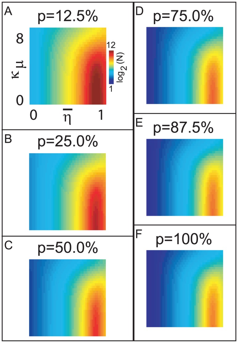
Given a network of the form described in the section entitled “A population-dynamics approach towards verifying Hypothesis 2 within more general networks”, with and fixed, one may ask if, for the LNI, the reliability of this LNI would decrease if the presynaptic-inhibitory strength were to be increased (while simultaneously decreasing so as to maintain the firing-rate ). Let us denote this condition by ‘hypothesis-2.1’. By analyzing the terms in the -order subnetwork-expansion, one can readily conclude that hypothesis-2.1 holds if the LNI does not presynaptically-inhibit its own ORN, and there is at least one other LNI which does presynaptically-inhibit the ORN. However, if the LNI presynaptically-inhibits its own ORN, then hypothesis-2.1 holds only if the size of the network is sufficiently large. This critical network size (above which hypothesis-2.1 holds with high probability) is a function of the background firing-rate of the ORNs , the strength of vesicle-depletion , and the sparsity-coefficient of the random network. In panel-A we plot , where we have calculated such that, for values of , a randomly selected LNI within an E-R random network generated with sparsity-coefficient is highly likely (probability 75%) to obey hypothesis-2.1, given that the LNI in question presynaptically-inhibits its own ORN. Values of are displayed according to the colorscale shown on the right. In the remaining panels B–F we plot for different values of . Note that, unless is small and is large, it is highly likely that hypothesis-2.1 holds (even for LNIs which presynaptically-inhibit their own ORNs) for all LNIs within an E-R random network of size .

This type of approach can also be used to analyze hypothesis-2.2. Using similar techniques as above, one can readily show that hypothesis-2.2 holds with high likelihood for all LNIs in an E-R random network of any size regardless of whether or not those LNIs presynaptically-inhibit their own ORNs, as long as their ORNs are presynaptically-inhibited by at least one other LNI.

Through the application of the above analysis, one can show that all sufficiently large E-R random networks obeying the dynamics of Eq. 16 have a high likelihood of satisfying the three properties associated with hypothesis-2 — namely, (0) there exists a -parameter family of network parameters ranging from type-A to type-B for which the firing rate of any particular LNI is maintained, (1) as the network parameters are shifted along this -parameter family in the type-A direction, that LNI's reliability decreases, and (2) as the network parameters are shifted along this -parameter family in the type-A direction, that LNI's sensitivity to its dedicated ORN channel increases. For the class of networks considered in Fig. 8 the critical above which hypothesis-2 holds is roughly . Although this critical value obtained from our idealized model should not be compared quantitatively with the number of LNIs in the real fly AL, we expect that a similar qualitative result should hold for more realistic models — namely that hypothesis-2 should hold for any model as long as the presynaptic-inhibitory network includes sufficiently many inter-glomerular connections and the number of LNIs is sufficiently large.

This type of subnetwork analysis can also be used to probe the relationship between connectivity and dynamics that exists in more complicated heterogeneous networks, including scale-free and small-world networks, as well as networks in which the different neurons are governed by different equations. In each case, one can use the distribution of subnetworks within the larger network to determine dynamical features associated with neurons inside that network. For example, one can easily show that, for a scale-free network obeying the dynamics specified in Eq. 16, if the ORN-LNI pair has low incoming-degree and is presynaptically-inhibited by ORN-LNI pairs with high incoming degree, then the LNI is likely to violate hypothesis-2.1. This is simply because there will be an overwhelming number of subnetworks of the form , which each contribute to the decrease of var when is scaled up (assuming as before that is appropriately decreased to maintain the firing-rate ).

Finally, before we conclude, we address the effect of excitatory interconnectivity in the AL, which was not taken into account in the simple model analyzed above. Let's assume for a moment that, in the above model, we had added excitatory cells (say, LNEs) which were also affected by the ORN input channels. When analyzing the effect of modifying on the LNIs, the excitatory interactions associated with the LNEs only come into play at the -order. For example, if indices correspond to LNIs and index corresponds to an LNE, the simplest coupling terms by which LNE- can affect LNI- are of the form . Similar to the -order contributions shown in Fig. 7, The contributions of this term are dwarfed by the contributions of the LNI-LNI terms and . When analyzing the effects of modifying on the LNEs themselves, the situation is similar, with excitatory interactions playing a secondary role to the dominant contribution of first-order presynaptic-inhibitory connections. Thus, as long as the number of LNIs which affect each AL-neuron is not much less than the number of LNEs which affect that neuron (and as long as excitation and inhibition have effects of comparable magnitude), we expect the analytical results of this section to hold for networks which include both excitatory and inhibitory neurons.

Discussion

Using our large-scale model for the fly antennal lobe, we have been able to put forth two hypotheses which concern the functional role played by synaptic-depression at the ORN synapses within the fly AL. The first of these hypotheses is that ORNAL synaptic-depression may contribute to a form of variance coding when ORN firing-rates are high. The second hypothesis is that two network mechanisms which both give rise to synaptic-depression (namely presynaptic-inhibition and vesicle-depletion) participate in establishing a balance between the network's reliability and sensitivity.

The first hypothesis hinges on the fact that, as ORN firing-rates increase beyond the value at which PN firing-rates saturate, the corresponding increase in ORNPN synaptic-depression diminishes the postsynaptic impact of each individual ORN firing-event. In many situations (e.g., when many ORNs stimulate each PN, and different ORNs fire independently of one another), this scenario directly implies that, as ORN firing-rates increase, the ratio between the variance in input to the PNs and the mean input to the PNs decreases. If the ORNPN synaptic-depression is sufficiently large, the variance in input to the PNs can actually decrease as ORN firing-rates increase, while the mean input to the PNs remains the same. When the variance to the PNs decreases sufficiently, the PNs behave as though they are driven by an input current. This current-like drive typically gives rise to very regular (periodically firing) PN dynamics. This first hypothesis is very general, and evidence of this hypothesis manifests in our simulations for a wide range of parameter values. As mentioned above, synaptic-depression (including vesicle-depletion and presynaptic-inhibition) is just one of several mechanisms which could contribute to this variance-coding effect.

One of the most straightforward predictions of our first hypothesis is that, within the real AL, the trial-to-trial variability of PN responses should decrease as ORN activity increases beyond the point where PN firing-rates have saturated. This should be measurable at the level of individual PN responses, as long as the odor stimuli are chosen at the appropriate concentrations (see, e.g., [18]). Many of the experimental protocols which are currently employed are sufficient to test this prediction.

If such a variance code is indeed found in the fly AL, then the next question is whether or not the fly makes use of it. There are many ways in which an appropriately constructed downstream neuronal system could discriminate between two different stimuli that give rise to PN activity with similar firing-rates but differing degrees of regularity. For example, a downstream neuron may be wired to a subset of PNs in a given glomerulus in such a manner that (i) the steady nearly-periodic sequence of PN firing events associated with low-variance high-firing-rate PN activity (observed when is very high) does not stimulate the downstream neuron sufficiently to induce firing, whereas (ii) the occasional clusters of PN firing-events which occur during high-variance high-firing-rate PN activity (observed when is not quite so high) do stimulate the downstream neuron to fire. This is one of many potential ‘readout’ mechanisms that could serve to discriminate amongst stimuli which generate high ORN firing-rates. Such a readout mechanism may be at work within Kenyon cells, which have been observed to act like coincidence detectors [26]–[28]. A Kenyon cell that has a ‘high-threshold’ for firing may function as a coincidence detector, while also responding preferentially to spike-clusters within high-variance high-rate PN activity, but not to low-variance high-rate PN activity. An illustration of this principle is given in Fig. 2H. There are many other potential readout mechanisms that could serve to detect changes in the variance of PN activity, and effective readout mechanisms are likely nonlinear in nature [29],[30].

Our first hypothesis may have significance for concentration-coding within the fly olfactory system. As an odor's concentration increases there are two typical changes to the ORN activity induced by that odor: (i) the number of activated ORN classes increases, and (ii) the ORN firing-rates within each activated class increase and eventually saturate [18], [31], [32]. It has been proposed that the firing-rates of the PN population across many glomeruli can collectively encode both stimulus identity and stimulus intensity [32]–[34], but it is still unclear how such a population firing-rate code could be deciphered by a downstream network within the fly. Our first hypothesis suggests an alternative to such a population firing-rate code, as the activity of a single glomerulus can also encode information regarding stimulus intensity, even when the glomerular firing-rates are saturated. Thus, a downstream decoder need not necessarily integrate information from multiple glomeruli in order to assess the intensity of a stimulus. In cases where a pair of high-concentration odors do in fact saturate the responses of most of the glomeruli which they target, typical readout mechanisms designed for rate-coding may not serve to discriminate these odors [35], and variance-coding mechanisms relying on transient bursts of activity (as mentioned above) may be more useful (see, for example, [36]).

The second hypothesis contains two statements. The first is that feedback-dominated synaptic-depression (i.e., presynaptic-inhibition) within type-A networks allows type-A networks to be more sensitive than type-B networks to shifts in input. Thus, type-A networks outperform type-B networks at odor-discrimination tasks when long observation-times are allowed. This statement seems to be true within our model network over a wide range of parameter values. The second statement is that feedforward-dominated synaptic-depression (i.e., vesicle-depletion) within type-B networks allows type-B networks to be more reliable than type-A networks (over multiple presentations of the same odor). This seems to be true within our large-scale model when (i) the typical number of ORN firing-events presynaptic to each PN within a glomerulus is larger than the typical number of LNI firing-events presynaptic to the ORNs which target that glomerulus, (ii) the vesicle-depletion experienced by the ORN synapses is relatively well stereotyped across ORN firing-events, and (iii) the presynaptic-inhibitory network includes many ‘inter-glomerular’ connections. These three conditions seem to hold for the fly AL [12], but in other situations these conditions may be violated, and the converse of this second statement may hold. For example, we conjecture that in a hypothetical system containing (i^′) very many high-firing-rate LNIs and PNs driven by only a few low-firing-rate ORNs and (ii^′) a vesicle-depletion mechanism that is highly variable from one ORN firing-event to the next, it is likely that LNIORN presynaptic-inhibition can control the ORN input to the PNs much more reliably than vesicle-depletion of the ORN synapses could. In this hypothetical system type-B networks would be quite unreliable. Furthermore, even in a system with many ORNs and few LNIs, if (iii^′) the presynaptic-inhibitory network is dominated by strong intra-glomerular connections (between LNIs and ORNs associated with the same odorant channel), then the subnetwork analysis carried out above indicates that type-A networks would actually be more reliable than type-B networks.

Obviously, the real AL for any given fly has a fixed architecture, and it does not seem likely that a fly could vary the effect of vesicle-depletion and presynaptic-inhibition on the ORN synapses to take advantage of a tradeoff between reliability and sensitivity. However, the hypothesis above does apply to the fly AL in the sense that fly physiology may be balanced to achieve some optimal compromise between gain (i.e., responsivity), reliability, sensitivity and discriminability over short observation-times.

Suggestions for future study

The intuition gained in this study may be useful for understanding the coding properties of olfactory systems in other insects, or even in mammals, many of which also exhibit synaptic-depression.

In the olfactory system of many other insects, such as the locust and honeybee, the antennal lobe activity is characterized by oscillations which develop soon after the onset of stimulus. These oscillations are thought to be a key feature of the AL-response in these animals [26], [33]. Since such oscillations do not manifest quickly in the fly [17], the dynamical regimes studied in this paper are not of this nature. However, we can retune our computational model to produce oscillations by increasing the density of lateral connectivity within the AL (thus, bringing our model closer in structure to that of [33]). The analytical techniques used in this paper may also be useful for studying some of the phenomena associated with such an oscillatory regime.

Within certain mammals, such as the mouse, primary olfactory input to the olfactory bulb can be presynaptically inhibited by interneurons [37]–[39]). Because the architecture of the mammalian olfactory system is different from that of the fly, the hypotheses investigated in this paper may not directly apply. For example, in the mouse it has been found that inhibitory neurons in the olfactory bulb strongly presynaptically-inhibit the olfactory sensory neurons stimulating their own glomerulus, but not those stimulating other glomeruli [40], a situation markedly different from the presynaptic-inhibitory network of the fly AL [12]. Thus, as hinted in (iii^′) above, one might expect type-A networks to be both more sensitive and more reliable than type-B networks in the mouse. The extra coding power afforded by ‘feedback-induced’ synaptic-depression in this scenario may be necessary for an animal which is forced to sample it's olfactory environment using short observation times (e.g., nose-pokes and sniffs). This sort of speculation begs for a more detailed investigation of the structural and dynamic mechanisms at work in the mammalian olfactory system.

Materials and Methods

Overview of large-scale point-neuron model

In this section we describe the point-neuron model we used to investigate the dynamics of the fly AL. This model incorporates glomerular channels, each with PNs, LNEs, LNIs and ORNs, and incorporates presynaptic-inhibition as well as vesicle-depletion (see Fig. 1). Each PN, LNE, LNI and ORN is modeled using single-compartment Hodgkin-Huxley type kinetics using standard sodium and potassium currents that give rise to fast sodium spikes [22] similar in shape to those observed experimentally [41].

Model synaptic currents

ORN, PN and LNE excitatory synapses and LNI GABAergic synapses are modeled by fast-activating synaptic currents [34], [42]. Excitatory and GABAergic transmission are both modeled via stereotyped instantaneous neurotransmitter release in response to a presynaptic action potential, with ORN synapses experiencing vesicle-depletion. Although there is evidence for a slowly activating inhibitory current in the honeybee [43], we are not aware of any similar evidence for such slowly activating inhibitory current in the fly AL. There is, however, evidence for both long-timescale GABA-B type inhibitory currents, as well as short-timescale GABA-A type inhibitory currents in the fly AL [11]. To account for these two timescales, both a long- and short-timescale inhibitory current are incorporated into this model — the relevant synaptic currents include fast excitation (nAch-type, timescale 5–10 ms), fast inhibition (gabaA-type, timescale 10–15 ms) and slow inhibition (gabaB-type, timescale 100–400 ms).

Model connectivity

Experimental observations indicate that all the ORNs that express the same odorant receptor gene have similar odor responses and project to the same glomerulus in the brain [18], [44]. Each PN receives direct ORN input from a single glomerulus [6], and thus all the ORNs and PNs corresponding to a given glomerulus constitute a discrete processing channel. We have designed the architecture of our model to reflect these experimental observations — our model ORNs and PNs only project to PNs and LNs associated with their own glomerulus.

Experimental observations also indicate that glomeruli are interconnected by a network of local interneurons. There have been several experimental results implying that the lateral connectivity between glomeruli in the AL has a strong inhibitory component, and that this inhibitory component is partly due to presynaptic-inhibition (i.e., LNIs synapsing on the ORN axons presynaptically) [12], [13], [41]. It has also been revealed that ORN-PN synapses are quite strong, and likely experience substantial synaptic-depression through vesicle-depletion [11]. Our computational model reflects these observations, and model LNEs and LNIs project to neurons both within and outside their own glomerulus. In addition, the model LNIs only affect the ORNs presynaptically. That is, deposition of neurotransmitter from LNIs onto ORNs only suppresses the efficacy of the synapse at the ORN axon (without suppressing the membrane potential at the ORN soma). In order to model vesicle-depletion, the efficacy of the synapse associated with each ORN is depleted each time that ORN fires [22].

There is debate as to whether or not there is a functionally relevant large-scale structure to the lateral connections within the AL, such as center-surround excitation/inhibition, or chemotopy [7], [45]. The lateral connectivity in our model network is structured so that the interconnections between ORNs, PNs, LNEs and LNIs are sparse and randomly determined. Thus, the results of our model may be expected to generalize to a variety of networks with a degree-distribution similar to that of an Erdos-Renyi random-graph. The connectivity of the network is encoded by a matrix , with labelling the existence of a connection between cell and cell . Each entry in the connectivity matrix is randomly chosen to be either or independently, with connection probabilities specific to the cell types and glomerular channel assignments of neurons and . Both the connection probabilities, as well as the coupling strengths are chosen in a manner consistent with the literature (details given in the sections regarding benchmarking below).

Model odor input

The model ORNs themselves are each stimulated by Poisson input. In background (i.e., in the absence of an odor stimulus) the Poisson input rate is 350 Hz, and the input strength is low enough that the ORN background firing-rate is , and the corresponding PN background firing-rate is (consistent with experimentally observed firing-rates — [6], [41]). Odor presentation within this network is modeled by stimulating the ORNs corresponding to a subset of glomerular channels (typically around half of the glomerular channels) with additional high-rate Poisson input, in addition to the background Poisson input (consistent with experiments which indicate that an odorant typically activates multiple ORN types and triggers activity in to of the glomeruli — [18], [20], [46], [47]). In this manner, a model odor is represented in a combinatorial fashion — an odor is defined by the degree to which that odor drives the various ORN input channels. To simulate odors of different chemical composition, we stimulate different subsets of ORN input channels, whereas to simulate odors of the same chemical composition (but of differing concentration) we stimulate the same input channels to differing degrees, as motivated by the observation that varying the concentration of a given odor tends to modulate the firing-rates of responding ORNs in vivo [45], [48]–[50]. The odor-dependent noisy input signal is sufficient to drive individual ORNs strongly stimulated by the odor to firing-rates of . We choose a time-course of the odor-specific ORN current stimulus that is comparable to the time-course observed experimentally [18]. Specifically, at the time of ‘odor onset’ we increase the input-specific drive to the ORNs slowly (over ), and at odor offset we decrease the input-specific ORN drive even more slowly (over ). While there is some evidence of more complicated odor-specific temporal structure to ORN odor response, we will model only the temporally simplistic ORN response detailed above, so as to focus on emergent dynamics within the AL which manifest solely as a result of AL interconnectivity.

Benchmarking the model

We have tuned the model so that, with a single set of parameters, the model exhibits a dynamic regime that is consistent with a variety of experimentally observed phenomena.

We attempted to ensure that the model network architecture is consistent with the literature. For example, motivated by [13], We chose the inhibitory postsynaptic coupling strengths from LNIsPNs so that the lateral inhibitory IPSC to a PN has both a fast and slow component (in our model IPSCs incorporate 50% fast (gabaA type) and 50% slow (gabaB type) inhibition). Similarly, we chose the inhibitory postsynaptic coupling strengths from LNIsLNEs and LNIsLNIs to be 100% fast-type. As another example, motivated by [41], we have chosen LNEPN intra-glomerular coupling to be sparse enough (15%-25%) to align with the fact that direct LNPN connections are rarely observed. Nevertheless, LNEPN inter-glomerular coupling is dense enough that lateral excitatory input is still observed between most pairs of glomeruli [8], [9]. The lateral excitation between glomeruli is sufficiently strong that, even when ORNs belonging to a particular glomerulus are removed, some PNs and LNs within that glomerulus can still fire after odor presentation.

Stimulus driven dynamic transients reflect PN reliability and saturation

We tuned the ORNPN connection probabilities and connection strengths in our model so as to produce stimulus-triggered dynamic transients which are qualitatively similar to experiment. This stimulated set of ORNs directly activates a corresponding subset of glomeruli. As the glomeruli respond to the ORN input, the glomerular activity pattern shifts and spreads to include other glomeruli not directly stimulated by the odor.

As shown in Fig. 9, the stimulus triggered firing-sequence of a typical model PN is more reliable than the corresponding sequence for a typical ORN associated with the same glomerulus, and the PN PSTH typically peaks after but before the ORN PSTH peaks (consistent with [20]). The sensitivity and reliability of PN activity within our model is critically dependent on three features: (i) the convergence ratio of ORNs to PNs must be sufficiently high that any given PN receives strong reliable input (summed over ORNs) immediately after odor onset, (ii) there must be some synaptic-depression at the ORN synapses, otherwise the PN activity does not peak before the ORN activity peaks (rather, the PN activity saturates and remains constant), and (iii) the combination of ORN activity and synaptic-depression at the ORN synapses must give rise to essentially ‘mean-driven’ (i.e., low-variance super-threshold) input to the PNs during odor presentation. These three network mechanisms seem to be necessary and sufficient to give rise to high-firing-rate PN activity which peaks prior to the peak in ORN activity, and which is more reliable than any single ORN's activity. We note that the source of synaptic-depression is not constrained by this particular phenomena — either vesicle-depletion or presynaptic-inhibition (generated by the recruitment of LNIs in other glomeruli) can give rise to mean-driven ORNPN input, and hence to reliable PN firing sequences. As shown in Fig. 10, the PN firing-rate is a nonlinear function of ORN firing-rate when averaged across odors and trials and PN/ORN pairs within any given glomeruli, as is consistent with experiment [20].

Figure 9. PNs are more reliable than their individual ORN inputs.

Shown are averaged response curves for a typical model PN (magenta, solid) and model ORN (green, dashed) associated with the same glomerulus in our model. The grey overlay indicates the odor presentation period. Spikes were counted in bins. The mean spike-count per bin (averaged over trials) is shown on the left. The standard-deviation in spike-count per bin is shown in the center, and the coefficient of variation (standard deviationmean) is shown on the right. Note that, qualitatively similar to experiment [20], the model PN activates more quickly, has higher firing-rates, and is more reliable than the ORN.

Figure 10. The relationship between ORN firing-rates and PN firing-rates is nonlinear.

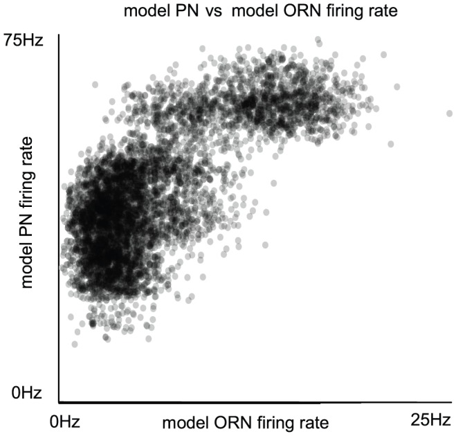
Shown is a scatterplot of model PN and model ORN firing-rates associated with a typical glomerulus in our model. Spike rates were measured during the epoch during which PN firing-rates peak following odor presentation. Note that, qualitatively similar to experiment [20], the model PN firing-rates saturate for relatively small values of ORN firing-rates.

PNs are more broadly responsive to odors than their ORN class would indicate

Experimentally, it has been observed that most PNs respond to multiple odors [45], [51], and are more broadly responsive than their input ORNs [9], [20] — there are many different PNs which respond to odors that do not stimulate their respective ORNs, and there are PNs which do not respond very strongly even when their respective ORNs are strongly stimulated. Thus, due to the lateral connectivity within the AL, the total set of activated glomeruli corresponding to a particular odor is generally not in one-to-one correspondence with the set of activated ORN olfactory receptors stimulated by that odor. Many believe that the inter-glomerular crosstalk is critically important for redistributing the glomerular activity within the AL ([41], but also see [7], [45]). It has been postulated that this re-expression of the odor at the glomerular level is advantageous for the fly, as the combinatorial code linking different odors to different glomerular subsets serves to separate similar odors more efficiently than the corresponding combinatorial code at the olfactory receptor level [20].

We tuned the lateral connection probabilities and connection strengths within our model to produce a dynamic regime capable of rich glomerular activation patterns which are qualitatively similar to experiment. As shown in Fig. 11, the lateral connectivity in our model is sparse enough that oscillations do not develop during the initial odor-response, and yet strong enough that the activity of PNs and LNs within each glomerulus is not in direct correspondence with the activity of their respective ORN inputs. This lack of correlation between PN response and ORN response across odors can be quantified by measuring the PN-PN and PN-ORN rank-correlation, which is in good qualitative agreement with experiment [20]. In our model, as in experiment, LN activity is similar to PN activity (data not shown). For example, LN firing-rate can get quite high, and typically peaks shortly after odor onset [13].

Figure 11. PNs exhibit broader odor responses than their associated ORNs.

[A] Shown are trial-averaged firing-rate curves for various model PNs (magenta, solid) and associated model ORNs (green, dashed) in response to various model odors. Note that, qualitatively similar to experiment [12], the activity of the model PNs does not necessarily reflect the activity of the associated model ORNs. [B] Shown are the PN-ORN (green) and PN-PN (red) Spearman rank-correlation histograms for the model PNs and associated model ORNs (averaged over all PN and ORN pairs associated with each given glomerulus, and then further averaged over glomeruli — see [20] for the statistical methods used). Note that, qualitatively similar to experiment, the mean of the PN-ORN histogram is closer to than the mean of the PN-PN histogram, indicating that, while PNs associated with a given glomerulus tend to respond to the same odors, they do not necessarily respond to the same set of odors which stimulate their associated ORNs.

ORNPN induced EPSCs attenuate as frequency of ORN synapse activation increases

Our model of vesicle-depletion and presynaptic-inhibition is phenomenological, and is intended to allow us to qualitatively reproduce and investigate the functional role of synaptic-depression at the ORN synapses. We have chosen a parsimonious model for vesicle-depletion, involving only one timescale of , and one parameter . Similarly, our model of presynaptic-inhibition involves only the timescales of synaptic inhibition and a coupling strength (see the section regarding vesicle-depletion and presynaptic-inhibition below). In order to ensure that our phenomenological model of synaptic-depression at the ORN synapses (a combination of vesicle-depletion and presynaptic-inhibition) was qualitatively accurate, we followed the experimental paradigm of [11]. We constructed a numerical experiment to measure the attenuation timescale of ORNPN input (see Fig. 12). We first forced the ORN synapses to activate periodically at (to simulate ORN background firing-rates), and then once the system equilibrated to this periodic input, we increased the frequency of ORN stimulation (to ) and measured the input current to each PN as a function of time. For a larger given frequency , the attenuation of the PN EPSC will occur more quickly. We tuned the coupling strengths so that the attenuation time scale (as a function of ) qualitatively matched experimental observations [11]. Our modeling work indicates that the attenuation time-scale match experiment as long as and are sufficiently high (the exact ratio of to is not strongly constrained by this particular experiment).

Figure 12. Synaptic-depression at the ORN synapses.

Shown are current traces associated with a model PN in response to direct current stimulation of the model ORNs associated with that PN. Analogous to experiment [11], the model ORNs associated with the model PN have been stimulated by periodic input current prior to the epoch shown in the figure. At the start of the epoch shown in this figure, the ORN stimulation is increased to , , , or . The trial-averaged model PN EPSCs in response these different stimulations are plotted (over a time interval of ). Above each EPSC curve, we show the envelope of the response in gray. This envelope is calculated by fitting a piecewise linear function to the maxima of the EPSC response sampled at the rate of stimulation. Note that, similar to experiment, the envelope of the PN EPSC attenuates more quickly when stimulated at than when stimulated at .

A further constraint on our model of synaptic-depression can be obtained by considering the correlation between total ORN activity, and reduction in subthreshold voltage observed at any given PN [12]. To obtain a roughly linear relationship between ORN activity and PN inhibition (as shown in Fig. 13), our model requires .

Figure 13. Presynaptic-inhibition is partly responsible for ORN PN synaptic-depression.

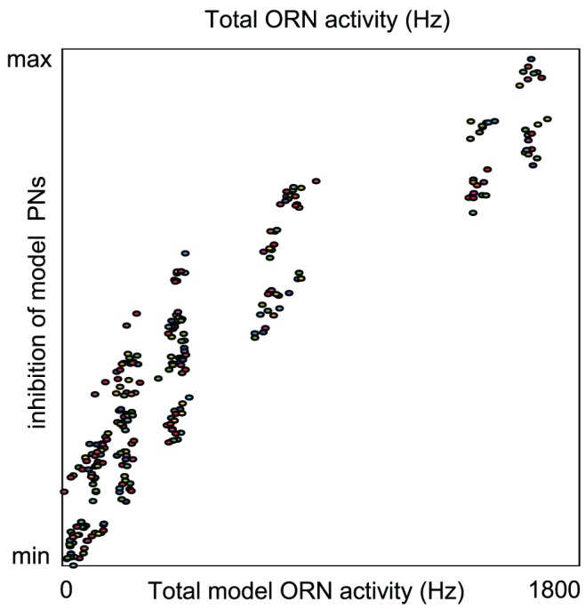
Shown is a scatterplot displaying the correlation between total ORN activity across all glomeruli in response to various odors, and the suppression of spontaneous EPSPs associated with a particular PN associated with a glomerulus which has been ‘shielded’ (i.e., the odor stimulus chosen does not affect the input drive to that glomerulus). In analogy with [12]. The PN suppression is measured as the difference in integrated PN membrane potential between (i) the scenario in which the PN receives spontaneous spikes from its associated ORNs in the absence of any odor, and (ii) the scenario in which the glomerulus associated with that PN is shielded and an odor is presented, in which case the activity generated within the other glomeruli reduce the effect of the spontaneous spikes impingent on the PN, and the spontaneous EPSPs are absent or greatly diminished. Note that, due to presynaptic-inhibition within the model, the correlation between PN EPSP magnitude and total ORN activity is qualitatively similar to experiment [12].

Details pertaining to Neuronal Model

The membrane potential of each ORN is governed by equations of the form

with stimulus current described in a section entitled “Odor Stimulation” below. The membrane potential for each PN, LNE and LNI is governed by equations of the form:

The parameters for the passive leak current are , , .

Intrinsic currents

The intrinsic currents for each neuron consist of fast sodium and potassium currents and . These currents obey equations of the following form:

The maximal conductances are , and . The reversal potentials are , .

The gating variables take values between and and obey equations of the following form:

and are described in [52]:

Synaptic currents

Given two connected neurons in the network, the synaptic conductances of the postsynaptic neuron are increased whenever the presynaptic neuron's membrane potential rises above a threshold of (i.e., when the intrinsic currents of the presynaptic neuron generate an action potential). The excitatory-synaptic current associated with the neuron in the network is governed by an equation of the following form:

(4)

(5)

with the excitatory reversal potential . The efficacy of the excitatory-type synapse associated with the neuron obeys the equation:

(6)

where , the times are the spiketimes of the neuron, , and (adapted from [33], [34], [53], [54]). The term represents synaptic-depression at the ORN synapses, and is used to model both vesicle-depletion and presynaptic-inhibition at these synapses. This term is identically if corresponds to a PN, LNE or LNI. The dynamics of when corresponds to an ORN will be discussed later. The differential equation Eq. 6 is structured so that for all time, and in the absence of firing . The synaptic GABA-A current for the PNs, LNEs and LNIs obeys equations analogous to Eqs. 4,6, with . The efficacy of the GABA-A-type synapse associated with the neuron obey the equation

(7)

with . The synaptic GABA-B current for the PNs, LNEs and LNIs obeys an equation of the following form:

with inhibitory reversal potential . The quantity for the neuron obeys the equation:

with . The efficacy of the synapse for the neuron obeys an equation analogous to Eq. 7, with . Thus, the slow GABA-B type synaptic current has a rise and decay time-scale, whereas the fast excitatory and GABA-A type synaptic currents only have decay time-scales (again adapted from [33], [34], [53], [54]).

The synaptic coupling strengths , , and depend only on the cell types of neurons and , and are chosen so that only presynaptic ORNs, PNs and LNEs give rise to excitatory-type currents, and only LNIs give rise to GABA-A and GABA-B-type currents. The strengths are given by the following arrays:

(8)

The parameter varies between (no presynaptic-inhibition) and (strong presynaptic-inhibition). Note that the PNPN and LNIPN coupling strengths are all negligible, to account for the experimental observations that PNs may not be targeted by other PNs, or by local inhibitory interneurons. However, we do allow for PNs to connect to LNEs (and LNIs), as observed in [41]. If these strengths are set to we can retune the remaining connectivity strengths so that our major conclusions still hold (data not shown).

Network connectivity

The intra-glomerular connection probabilities are given by the array:

(9)

and the inter-glomerular connection probabilities are given by the array:

(10)

Modeling vesicle-depletion and presynaptic-inhibition at the ORNPN and ORNLN synapses

The ORNs in this model do not directly experience synaptic conductances from either the PNs or the LNEs. The excitatory-type from PNs and LNEs onto ORNs is identically (see the array shown in (8) above). The GABA-A and GABA-B-type conductances associated with an ORN (say, with index ) alter the term in Eq. 6, thus affecting the efficacy of synapses from the ORN onto the AL. The evolution of in our model is governed by two parameters: (described above), and (described below). These two parameters will allow us to consider a -parameter family of model networks in which the strength of vesicle-depletion and presynaptic-inhibition can be altered independently (see Fig. 4). The equations governing the evolution of are

with the vesicle-depletion parameter obeying the differential equation:

with . The parameter varies from (no vesicle-depletion, ) to (complete vesicle-depletion with each firing-event). As the vesicle release rate per synaptic event is likely quite high within the real fly AL [11], values of are most reasonable from a physiological standpoint. Note that the vesicle-depletion parameter is bounded between and .

Odor simulation

The stimulus current to the ORN is governed by the equation

where is a response-function such that if , and if , with . The spiketimes are drawn from a Poisson-process with rate . The strength of this background input is . The spiketimes are drawn from a Poisson-process with rate which depends on the time since odor onset, the odor being presented, as well as the ORN under consideration. Typical values for range from (when the odor does not directly stimulate the ORN) to (when the ORN is being strongly stimulated by the odor). The strength of this odor-specific input is .

The time-dependence of the odor-specific input-rate is governed by the factor

with and representing the onset and offset times of the odor stimulus (respectively), and with , . A typical odor (stimulation of the ORNs within of the glomerular channels) activates of the PNs, which fire at about . Not all of the PNs exhibit increased activity upon odor stimulation — a given odor will typically cause a few PNs which are not directly stimulated to actually decrease in activity (as a result of inter-glomerular inhibition). On presentation of a typical odor, the typical PN PSTH rises very quickly, and peaks after , before the ORN PSTH peaks (at by construction). The typical PN PSTH decays more quickly than the ORN PSTH ( vs ms). Due to lateral connectivity, PNs respond to a broader selection of odors than their ORN inputs and most PNs have a ‘rank order’ of odors that is different from the rank order of their ORN inputs. Note that PNs exhibit a rise in firing-rate after odor offset only very rarely. This is a consequence of the fact that the current model only incorporates odors which increase the firing-rate of the stimulated ORNs. It has been observed that some odors actually decrease the firing-rate of certain ORN types, with perhaps a resurgence of ORN firing-rates after odor offset (as shown in DL1 response to cis-3-hexen-1-ol, cyclohexane and ethyl acetate — [20]). These types of inhibitory OdorORN responses could potentially give rise to richer PN dynamics (potentially triggered by PNs/LNs which fire greatly after odor offset), and these phenomena will be studied in more detail in future work.

Odor discrimination

In order to estimate the model network's ability to discriminate different odors, we measure the odor-dependent probability distribution of each PN's firing-rate, and use standard methods from classification theory [55]. For completeness we describe our procedure applied to firing-rate vectors.

Assume that we are estimating the network's ability to discriminate between different odors. For each , we perform multiple trials of odor , and estimate the probability distribution

Once the are sufficiently well estimated, we perform and classify individual odor trials. A single trial of odor (randomly chosen to be either or with probability) will give rise to a vector such that is the number of firing-events produced by the PN during that trial. By looking at a fixed and comparing and , we can use the PN to identify a possible candidate stimulus (either odor if , or odor if ). This process can be performed for each , and in this way each PN ‘votes’ for a candidate stimulus. We tally these votes, weighting each one by the log of the information ratio associated with each PN. We use the weighting

where is the ‘hit-rate’ associated with the PN:

and is the ‘error-rate’. This particular weighting is chosen so that votes for stimulus with error-rate have the same combined weight as a single vote for stimulus with a far smaller error-rate of . The sum of the weighted votes is compared to determine the candidate stimulus underlying this particular trial. If the candidate stimulus matches the true stimulus, the trial is classified correctly. If not, the trial has been classified incorrectly. By going through this process with multiple trials, we can generate a probability that any given trial will be classified correctly. To perform -way discriminability tasks, we go through an analogous procedure, performing all pairwise discriminability tasks for each sample observation, and ultimately selecting the candidate stimulus corresponding to the majority (with ties automatically counted as incorrect).

We have chosen this particular procedure because it allows us to take advantage of components of the firing-rate vector which carry substantial information (as measured by the information ratio), without requiring an estimate of the joint distribution of firing-rates (across PNs) for any particular odor. Thus, this measure of discriminability is more sensitive than typical linear discriminators which use the Euclidian distance between firing-rate vectors (see [20]), but does not succumb to the curse of dimensionality associated with the large number of distinct PNs.

An idealized model used to illustrate variance coding

Here we describe in detail the idealized model used in the section entitled “A simple cartoon of variance coding” in the main text. This model includes a single conductance-based integrate-and-fire PN, driven by a set of ORNs, each endowed with a simple model of synaptic-depression. Each of the ORNs is modeled as a Poisson process with fixed rate ( ). The coupling strength between the ORNs and the PN is modulated by a term (), which is intended to model vesicle-depletion at the ORN synapses. As each ORN fires, this term will give rise to synaptic-depression between the ORNs and the PN.

The membrane potential and conductance for this single PN obey the following differential equations:

where , is the reset potential, is the excitatory reversal potential, and is the conductance time-constant. The voltage evolves continuously until reaches a threshold , at which point the PN fires, and is reset to . The conductance evolves continuously except when an ORN (say, the ORN) spikes, at which point jumps. The time is the spiketime of the ORN, and is the coupling strength associated with the ORN at time . If , the synapses between the ORN and the PN are exhausted. If , the synapses between the ORN and the PN are completely refreshed. For this simple model , and the equation for is given by:

where is the time-constant associated with vesicle-depletion. The term decays to continuously, except when the ORN fires at some time , at which point jumps by an amount proportional to (the limit is used since is not technically defined). The parameter governs the relative increase in associated with each spike , and hence is bounded between and . The parameters , and are chosen to be consistent with typical point-neuronal models, and the parameter is chosen essentially arbitrarily (different choices for do not qualitatively change the results).

A simple analyzable cartoon of variance coding

As a simple cartoon which illustrates Hypothesis 1, consider a single PN modeled by a conductance-based integrate-and-fire neuron [22], driven by a single ORN modeled as a Poisson process (with firing rate ). The state variables of the PN are the membrane-potential , the excitatory conductance , and the vesicle-depletion parameter . The equations governing the state of the PN are

(11)

where is the leakage conductance, is the reset potential, is the excitatory reversal potential, and is the conductance time-constant. The voltage evolves continuously until reaches a threshold , at which point the PN fires, and is reset to . The conductance decays to continuously except when the ORN fires. The time is the spiketime of the ORN, and is produced by a Poisson process with rate ., The conductance jumps by at time (the limit is used since is not technically defined). The vesicle-depletion parameter decays to continuously with time-constant , except when the ORN fires, at which point jumps by . In this simple model the vesicle-depletion parameter and conductance are both bounded to lie within . As the vesicle-depletion parameter increases, the effect of ORN spikes on the PN conductance decreases. It should be noted that the functional form for the ORNPN synapse — in this case modeled by — is chosen to make the subsequent analysis easier, and is not particularly realistic (as very small values for imply a very strong ORNPN synapse). Nevertheless, the general picture implied by this cartoon holds for more realistic models of vesicle-depletion (see the section entitled “A simple cartoon of variance coding” in the main text).

The simple model Eq. 11 can be analyzed by considering the long-time evolution of the PN. For sufficiently small , , and sufficiently large (with fixed), it can be shown [56] that the equilibrium-distribution of (collected by sampling over a sufficiently long time interval) is well-approximated by a Gaussian, with mean and standard-deviation given by:

It can also be shown that, under these conditions, the equilibrium-distribution of is also well-approximated by a Gaussian, with mean and standard-deviation given by:

Using the expression for , the expressions for and can be simplified to

Thus, for a sufficiently small , as the variance of equilibrium-distribution shrinks to , and the mean remains constant. Thus, as , the long-time conductance-distribution becomes sharply peaked around ; so much so that, for sufficiently large , the PN effectively has a fixed excitatory-conductance and will fire perfectly regularly with a period of

The excitatory conductance is, in this case, independent of the activity of the PN because the ORN input is only affected by vesicle-depletion, and not by presynaptic-inhibition. Nevertheless, the conclusions we draw from this simple model are quite general, and will hold for more realistic models of synaptic-depression.

Note also that synaptic-depression is critical to hypothesis-1 within this model. If were fixed to be (i.e., no synaptic-depression of the ORN synapses), and were sufficiently large, then the equilibrium-distribution of would be Gaussian with a mean and variance that grow unbounded as .

A simple model illustrating the tradeoff between reliability and sensitivity

In this section we analyze the model used in the section entitled “A simple analyzable cartoon of the tradeoff between reliability and sensitivity”.

To analyze the solutions of Eq. 1, let's assume for the moment that , and (i.e., neuron fires more frequently than neuron ). If , then and do not affect one another. The steady-state firing-rate of neuron is , and the steady-state firing-rate of neuron is . Let us define and . Since both and are perfect phase-oscillators, and fire perfectly regularly every and time-units (respectively). If there is a difference in ORN inputs to these two neurons (say, ), then the difference in firing-rates is . Thus, if , this system is perfectly reliable (in the sense that the ISI distribution of and the ISI distribution of both have variance), and somewhat sensitive to shifts in the input (in the sense that any difference in input is reflected in the difference of the output firing-rates).

If , then and affect one another with several consequences: (i) the steady-state firing-rates and will be lower than and (respectively), (ii) the ISI distributions of and will have nonzero variance, and (iii) the difference in steady-state firing-rates will be greater than . Indeed, as increases away from the system becomes less reliable while becoming more sensitive to shifts in the input. More specifically, for a given fixed , the system will settle down to a steady-state dynamics in which neuron fires either or times in between each pair of -firing-events. The steady-state sequence of spike-times is independent of the initial state of the network and, while not generally periodic, can be solved for explicitly.

To show why this is true, we consider the return-maps and . We define the return-map as follows: given a spike of neuron (say, ), let be the first spike of neuron which occurs after , and let be the first spike of neuron which occurs after — we define . Similarly, given a spike of neuron , let be the first spike of neuron after , and let be the first spike of neuron after — we define . For the return map , we can also define the numbers and as follows: is the number of times fires in between and , and is the number of times fires in between and . Similarly, for the return map , we can define as the number of times fires in between and , and as the number of times fires in between and . See Fig. 14 for an example of these return maps.

Figure 14. A simple analyzable cartoon of the tradeoff between reliability and sensitivity.

[A] Shown is a schematic of the simple network, consisting of 2 ORNLNI pairs, each of which presynaptically inhibits the other. [B] Shown on top are sample voltage-traces for the two LNIs (represented by and ) for the case . Shown on the bottom are sample voltage-traces for the two LNIs in the case that is nonzero. Note that after LNI A fires, is constant for -time. Similarly, after LNI B fires is constant for -time. A pair of voltages for LNI B are circled. This pair of voltages corresponds to a point on the graph of the return map , namely . For this point on the graph of , , and . [C] Shown on the top and bottom are return maps for the values , and , respectively. [D] Shown on the top and bottom are return maps for the values , and , respectively.

Recall that, without loss of generality, we have assumed . By considering the return maps and , one can easily show that the maximum and minimum of are and , respectively, and that the maximum and minimum of are and , respectively. Moreover, maps the interval into . Similarly, maps the interval into . It is straightforward to show that the image of under is composed of sub-intervals: (i) an interval of length for which , and (ii) an interval of length for which . Similarly, the image of under is composed of sub-intervals: (i) an interval of length for which , and (ii) an interval of length for which . Letting

(12)

one can show that the lengths and are given by

(13)

For both the sub-maps and the number of extra spikes . These observations allow us to conclude that the steady-state ISI distribution for neuron (i.e., ) has a peak of magnitude at , and a peak of magnitude at . Similarly, the steady-state ISI distribution for neuron (i.e., ) has a peak of magnitude at , and a peak of at . The steady-state firing-rates associated with these ISI-distributions can be expressed in closed form and directly computed:

(14)

Similarly, the means and variances associated with these steady-state ISI-distributions can be expressed in closed form (see Fig. 5).

By considering these expressions for small , one can see that the steady-state return-map consists of segments of length and , corresponding to inter-spike-intervals for neuron of length and , respectively. Thus, has distinct peaks (at and , respectively), and as increases the distance between these two peaks increases. As a consequence, as increases, the variance in increases. In effect, a larger implies that extra spikes from have a larger effect on the of . A similar argument applies to and , and one can also show that, as increase the difference in firing rates also increases (see Fig. 5). Thus, within this simple network, presynaptic-inhibition between the neurons disrupts their natural regularly-firing behavior, and increases the variance of their ISI distribution (thus decreasing their reliability).

In the discussion above, we assumed that . If we assume , we can express the system firing-rate in closed form as a function of , (simply by replacing with and with in Eqs. 12,13,14). By requiring the system firing-rate to be constant, we can define implicitly (as a function of ,, and the system firing-rate ). Thus, we can directly compute the -parameter family of networks which, for fixed ,, attain a fixed system firing-rate . As shown in Fig. 5, this -parameter family of networks does indeed range from type-A networks (with high and low ) to type-B networks (with low and high ). Moreover, as one moves along this -parameter family of networks by increasing (and decreasing appropriately), the variance in and increases, and the sensitivity also increases. In conclusion, this simple network illustrates that presynaptic-inhibition is capable of increasing the variance of the ISI distributions of the neurons within that network (hence reducing their reliability), while at the same time increasing the sensitivity of the neurons' firing-rates to subtle shifts in input.

Analysis of signal-to-noise ratio in a general discrimination task

In this section we provide details regarding the analysis in the section entitled “A simple cartoon of optimizing discriminability over short observation-times”. Our goal is to determine from a measurement whether the input to the system is or . Let us denote by and the mean and variance of . As long as is sufficiently large, the estimate can be considered to be drawn from . Thus, as long as is sufficiently large, the measurement can be considered to be drawn from (since ). If we attempt to discriminate between the two possible inputs by using a linear-classifier, then the error associated with the best linear-classifier is simply given by the overlap of the distributions and . Because and for this simple scenario, and the variance of these distributions is very similar for (see Fig. 5), the error is well-approximated by

where is the difference in the means of and , and is the average variance of and .

A discrete state model used to analyze hypothesis-2 within general networks with arbitrary architecture

In this section we describe the point-neuron model used in the section entitled “A population-dynamics approach towards verifying Hypothesis 2 within more general networks”. This model is a stripped down version of the fly AL, consisting of discrete-state LNIs, each driven by a different ORN. We will model each ORN-LNI pair as a discrete-state discrete-time Markov process which is as simple as possible, while still retaining the following features: (i) each LNI generates spikes, (ii) each ORN input spike contributes to the vesicle-depletion of that ORNLNI synapse, and (iii), each LNI spike gives rise to presynaptic-inhibition of ORNLNI synapses. We will model the ORN-LNI pair using the state-variables , and which represent LNI membrane-potential, ORN vesicle-depletion and ORN presynaptic-inhibition, respectively.

At each discrete time, each state variable is either or , thus, at each time, the ORN-LNI pair is in one of states. The input from the ORN to the LNI is modeled as a bernoulli-random-variable , which is with probability (and otherwise). The state-variables undergo transitions of the following form: , , , where

(15)

and the function is the logistic function

For this system and are the typical persistence times of the and states (respectively), and we will assume that . The state is considered a ‘firing’ state for LNI . If , then always equals . If and the LNI does not receive input (i.e., ), then . However, if and , then may transition to the firing state. Given that , the probability of transitioning from to the firing-state is typically , but is lowered if either or . The vesicle-depletion parameter is likely to transition to the state whenever the LNI receives input (i.e., ). The presynaptic-inhibition parameter is likely to transition to the state whenever many other LNIs in the network fire. Note that the connectivity matrix encodes the connectivity of the network, and can be chosen to encode many different network architectures (e.g., a densely connected homogeneous network, or a sparsely connected heterogeneous network). If is nonzero, then the LNI presynaptically-inhibits the ORN, making it more likely that , and thus less likely that ORN input from the ORN to the LNI will cause the LNI to fire. For this model are the overall strengths of vesicle-depletion and presynaptic-inhibition. As increases, the likelihood of transitioning to the state increases. Similarly, as increases, the likelihood of transitioning to the state increases as long as for some . Ultimately, we will assume that the probability that the neuron will transition from the state  = {, , } at time to the state  = {, , } at time is given by

(16)

Note that is an state-transition matrix which depends on the state of the neuron in the system as long as .

Analysis of reliability and sensitivity using a subnetwork expansion

This section reviews a diagrammatic approach to analyzing network dynamics, and presents the salient calculations relevant to analyzing ISI-distribution and firing-rate (which can then be used to analyze reliability and sensitivity, respectively). One way to understand the equilibrium dynamics of a network such as Eq. 15 is to first picture the network as a point in phase-space , with the network's current state determined by the collection of parameters

at the current time, where we denote by the state of the ORN-LNI pair. As time passes this network will trace out a trajectory in phase-space, and this trajectory will depend on the network's architecture (i.e., , , , ). If one could determine the ‘typical’ phase-trajectories exhibited by this network (over very long times) then, in particular, one could determine this network's spike-time reliability. If one could determine how this network's typical trajectories shift as the input changes, then one could determine this network's sensitivity. The typical trajectories of a network can be determined by considering both the evolution-operator of the network , and the frequency with which the network visits each part of phase-space (i.e., the network's equilibrium-distribution). The full evolution-operator is the probability that the network moves from state to state over one timestep. In this case is an matrix such that each entry has the form

The probability that the network will be in state at time , given that the network was in state at time is

(17)

Eq. 17 can be thought of as an integral over all possible paths in state-space connecting to (i.e., each path traverses the system-states , , …, in sequence). The equilibrium-distribution is an eigenfunction of with eigenvalue — namely

and in this case is an matrix (i.e., an -dimensional vector). In this discussion we will assume that is unique (i.e,. only has a single equilibrium-distribution). Note that both and are functions of the network's architecture.

Given both and , one can determine many properties of the network's equilibrium dynamics. For example, the probability that the neuron fires at any given time (i.e., the steady-state firing-rate of the neuron) is given by

where is a operator such that , except for states in which , in which case (i.e., ). Similarly, the probability that the neuron fires at times and , without firing at any intermediate times (denoted by ) is given by

where is a operator such that . The sensitivity of the network's firing-rates can be calculated via the derivatives . The reliability var of the neuron in the network can be characterized by calculating the variance of (considered as a distribution with respect to ).

Ideally, one might wish to determine how dynamic sensitivity (i.e., ) and reliability (i.e., var) vary as functions of a network's architecture. Unfortunately, the explicit functional dependence of and on architectural parameters (such as , , , ) cannot be directly determined for most typical networks. However, it is possible to approximate these quantities by considering a weak-coupling expansion of and in terms of .

If , then each ORN-LNI pair is independent from the rest of the network, and the full state-evolution operator can be constructed by taking an operator-direct-product of the various , where is the -dimensional state-evolution operator associated with the ORN-LNI pair shown in Eq. 16 (note that if , then each is independent of all other neurons). Similarly, if the full equilibrium-distribution can be constructed by taking the product of the various , where is the -dimensional equilibrium-distribution of the ORN-LNI pair (note that is the eigenvector of with eigenvalue ). Both and only depend on and . The sensitivity and reliability for this uncoupled network can be determined simply by computing the sensitivity and reliability for individual (uncoupled) ORN-LNI pairs.

If is small, then the network's full state-evolution operator is no longer a direct product of the (and is no longer a product of the ). Nevertheless, by taking a Taylor-expansion of in terms of (around ) one can approximate and via a series

It can be shown that the -order terms in these series (corresponding to and ) incorporate subnetworks of the original network spanning up to ORN-LNI pairs [24], [25]. Specifically, the -order terms capture the equilibrium dynamics of each single ORN-LNI pair in the absence of the rest of the network. The terms capture the first-order corrections associated with a single presynaptic-inhibitory connection of the form . The terms capture both the second-order corrections associated with a single presynaptic-inhibitory connection (of the form ), as well as the second-order corrections associated with presynaptic-inhibitory connections (of the form ). In the main text (Fig. 7), we have grouped the -order terms corresponding to only presynaptic-inhibitory connection with the -order terms associated with that connection. For example, when presenting the term associated with the subnetwork , we implicitly include both the -order term proportional to , as well as the -order term proportional to . When presenting the term associated with the subnetwork , we implicitly include both the -order term proportional to , as well as the -order term proportional to .

Using the series-expansion for and , one can compute a series-expansion for many quantities of interest (e.g., firing rate , autocorrelation , sensitivity or reliability var) in terms of subnetworks of the original network. One attractive feature of this approach is that the formal series-expansion can be constructed without specifying the connectivity matrix . The terms of the series expansion can then be analyzed to determine which connectivity matrices will give rise to various dynamic phenomena. As an example, the terms and in the series expansion for can be written as:

where we use the notation that is equal to the single-neuron operator shown in Eq. 16, with , and is the derivative of with respect to (the coupling parameter which appears in ). We also use the operator

In the above representation of and , we use to denote an operator-direct-product, and to denote an accumulation of operator-direct-products (analogous to the use of ‘’ and ‘’ respectively).

Funding Statement

This study was funded by the NSF. The funders had no role in study design, data collection and analysis, decision to publish, or preparation of the manuscript.

References

- 1. Axel R (1995) The molecular logic of smell. Sci Am 273: 154–159. [DOI] [PubMed] [Google Scholar]
- 2. Hildebrand J, Shepherd G (1997) Mechanisms of olfactory discrimination: converging evidence for common principles across phyla. Annu Rev Neurosci 20: 595–631. [DOI] [PubMed] [Google Scholar]
- 3. Vosshall L, Wong A, Axel R (2000) An olfactory sensory map in the fly brain. Cell 102: 147–159. [DOI] [PubMed] [Google Scholar]
- 4. Gao Q, Yuan Y, Chess A (2000) Convergent projections of Drosophila olfactory neurons to specific glomeruli in the antennal lobe. Nat Neurosci 8: 780–785. [DOI] [PubMed] [Google Scholar]
- 5. Treloar H, Feinstein P, Mombaerts P, Greer C (2002) Specificity of glomerular targeting by olfactory sensory axons. J Neurosci 22: 2469–2477. [DOI] [PMC free article] [PubMed] [Google Scholar]
- 6. Couto A, Alenius M, Dickson B (2005) Molecular, anatomical, and functional organization of the Drosophila olfactory system. Curr Biol 15: 1535–1576. [DOI] [PubMed] [Google Scholar]
- 7. Root C, Semmelhack J, Wong A, Flores J, Wang J (2007) Propagation of olfactory information in drosophila. Proc Natl Acad Sci U S A 104: 11826–11831. [DOI] [PMC free article] [PubMed] [Google Scholar]
- 8. Olsen S, Bhandawat V, Wilson R (2007) Excitatory interactions between olfactory processing channels in the Drosophila antennal lobe. Neuron 54: 89–103. [DOI] [PMC free article] [PubMed] [Google Scholar]
- 9. Shang Y, Claridge-Chang A, Sjulson L, Pypaert M, Miesenbock G (2007) Excitatory local circuits and their implications for olfactory processing in the fly antennal lobe. Cell 128: 431–432. [DOI] [PMC free article] [PubMed] [Google Scholar]
- 10. Stocker R, Lienhard M, Borst A, Fischbach K (1990) Neuronal architecture of the antennal lobe in drosophila melanogaster. Cell Tissue Res 262: 9–34. [DOI] [PubMed] [Google Scholar]
- 11. Kazama H, Wilson R (2008) Homeostatic matching and nonlinear amplification at identified central synapses. Neuron 58: 401–413. [DOI] [PMC free article] [PubMed] [Google Scholar]
- 12. Olsen S, Wilson R (2008) Lateral presynaptic-inhibition mediates gain control in an olfactory circuit. Nature 452: 956–960. [DOI] [PMC free article] [PubMed] [Google Scholar]
- 13. Wilson R, Laurent G (2005) Role of GABAergic inhibition in shaping odor-evoked spatiotemporal patterns in the Drosophila antennal lobe. J Neurosci 25: 9069–9079. [DOI] [PMC free article] [PubMed] [Google Scholar]
- 14. Vickers N, Baker T (1996) Latencies of behavioral response to interception of filaments of sex pheromone and clean air influence flight track shape in heliothis virescens males. J Comp Physiol A 178: 831–847. [Google Scholar]
- 15. Bhandawat V, Maimon G, Dickinson M, Wilson R (2010) Olfactory modulation of flight in drosophilais sensitive, selective and rapid. J Exp Bio 213: 3625–3635. [DOI] [PMC free article] [PubMed] [Google Scholar]
- 16. Lei H, Riffell J, Gage S, Hildebrand J (2009) Contrast enhancement of stimulus intermittency in a primary olfactory network and its behavioral significance. J Bio 8: 21. [DOI] [PMC free article] [PubMed] [Google Scholar]
- 17. Tanaka N, Ito K, Stopfer M (2009) Odor-evoked neural oscillations in drosophila are mediated by widely branching interneurons. J Neurosci 29: 8595–8603. [DOI] [PMC free article] [PubMed] [Google Scholar]
- 18. Hallem E, Ho M, Carlson J (2004) The molecular basis of odor coding in the drosophila antenna. Cell 117: 965–979. [DOI] [PubMed] [Google Scholar]
- 19. Nagel K, Wilson R (2011) Biophysical mechanisms underlying olfactory receptor neuron dynamics. Nature Neurosci 14: 208–218. [DOI] [PMC free article] [PubMed] [Google Scholar]
- 20. Bhandawat V, Olsen S, Schlief M, Gouwens N, Wilson R (2007) Sensory processing in the drosophila antennal lobe increases the reliability and separability of ensemble odor representations. Nat Neurosci 10: 1474–1482. [DOI] [PMC free article] [PubMed] [Google Scholar]
- 21. Olsen S, Bhandawat V, Wilson R (2010) Divisive normalization in olfactory population codes. Neuron 66: 287–299. [DOI] [PMC free article] [PubMed] [Google Scholar]
- 22.Dayan P, Abbott L (2001) Theoretical Neuroscience. Cambridge, MA: MIT press.
- 23. Masse N, Turner G, Jefferis G (2009) Olfactory information processing in drosophila. Curr Bio 19: R700–R713. [DOI] [PubMed] [Google Scholar]
- 24. Rangan A (2009) Diagrammatic expansion of pulse-coupled network dynamics in terms of subnetworks. Phys Rev E 80: 036101. [DOI] [PubMed] [Google Scholar]
- 25. Rangan A (2009) Diagrammatic expansion of pulse-coupled network dynamics. Phys Rev Lett 102: 158101. [DOI] [PubMed] [Google Scholar]
- 26. Perez-Orive J, Bazhenov M, Laurent G (2004) Intrinsic and circuit properties favor coincidence detection for decoding oscillatory input. J Neurosci 24: 6037–6047. [DOI] [PMC free article] [PubMed] [Google Scholar]
- 27. Wang Y, Guo H, Pologruto T, Hannan F, Hakker I, et al. (2004) Stereotyped odor-evoked activity in the mushroom body of Drosophila revealed by green fluorescent protein-based ca2+ imaging. J Neurosci 24: 6507–6514. [DOI] [PMC free article] [PubMed] [Google Scholar]
- 28. Turner G, Bazhenov M, Laurent G (2008) Olfactory representations by drosophila mushroom body neurons. J Neurophys 99: 734–746. [DOI] [PubMed] [Google Scholar]
- 29. Shamir M, Sompolinsky H (2004) Nonlinear population codes. Neural Comput 16: 1105–36. [DOI] [PubMed] [Google Scholar]
- 30. Barak O, Tsodyks M (2006) Recognition by variance: learning rules for spatiotemporal patterns. Neural Comput 18: 2343–58. [DOI] [PubMed] [Google Scholar]
- 31. Sachse S, Galizia G (2003) The coding of odour-intensity in the honeybee antennal lobe: local computation optimizes odour representation. Eur J Neurosci 18: 2119–2132. [DOI] [PubMed] [Google Scholar]
- 32. Ito I, Bazhenov M, Ong R, Raman B, Stopfer M (2009) Frequency transitions in odor-evoked neural oscillations. Neuron 64: 629–706. [DOI] [PMC free article] [PubMed] [Google Scholar]
- 33. Bazhenov M, Stopfer M, Rabinovich M, Abarbanel H, Sejnowski T, et al. (2001) Model of cellular and network mechanisms for odor-evoked temporal patterning in the locust antennal lobe. Neuron 30: 569–581. [DOI] [PMC free article] [PubMed] [Google Scholar]
- 34. Bazhenov M, Stopfer M, Rabinovich M, Huerta R, Abarbanel H, et al. (2001) Model of transient oscillatory synchronization in the locust antennal lobe. Neuron 30: 553–567. [DOI] [PMC free article] [PubMed] [Google Scholar]
- 35. Luo S, Axel R, Abbot L (2010) Generating sparse and selective third-order responses in the olfactory system of the fly. Proc Natl Acad Sci U S A 107: 10713–8. [DOI] [PMC free article] [PubMed] [Google Scholar]
- 36. Lei H, Christensen T, Hildebrand J (2002) Local inhibition modulates odor-evoked synchronization of glomerulus-specific output neurons. Nat Neurosci 5: 557–565. [DOI] [PubMed] [Google Scholar]
- 37. Wachowiak M, Cohen L (1999) Presynaptic inhibition of primary olfactory afferents mediated by different mechanisms in lobster and turtle. J Neurosci 19: 8808–8817. [DOI] [PMC free article] [PubMed] [Google Scholar]
- 38. Wachowiak M, McGann J, Heyward P, Shao Z, Puche A, et al. (2005) Inhibition of olfactory receptor neuron input to olfactory bulb glomeruli mediated by suppression of presynaptic calcium influx. J Neurophysiol 94: 2700–2712. [DOI] [PMC free article] [PubMed] [Google Scholar]
- 39. Pirez N, Wachowiak M (2008) In vivo modulation of sensory input to the olfactory bulb by tonic and activity-dependent presynaptic inhibition of receptor neurons. J Neurosci 28: 6360–6371. [DOI] [PMC free article] [PubMed] [Google Scholar]
- 40. McGann J, Pirez N, Gainey M, Muratore C, Elias A, et al. (2005) Odorant representations are modulated by intra- but not interglomerular presynaptic inhibition of olfactory sensory neurons. Neuron 48: 1039–1053. [DOI] [PubMed] [Google Scholar]
- 41. Wilson R, Turner G, Laurent G (2004) Transformation of olfactory representations in the Drosophila antennal lobe. Science 303: 366–370. [DOI] [PubMed] [Google Scholar]
- 42. Patel M, Rangan A, Cai D (2009) A large scale model of the locust antennal lobe. J Comp Neurosci in press. [DOI] [PMC free article] [PubMed] [Google Scholar]
- 43. Barbara G, Zube C, Rybak J, Gauthier M, Grunewald B (2005) Acetylcholine, GABA and glutamate induce ionic currents in cultured antennal lobe neurons of the honeybee, Apis mellifera. J Comp Physiol A 191: 823–836. [DOI] [PubMed] [Google Scholar]
- 44. Clyne P, Grant A, O'Connell R, Carlson J (1997) Odorant response of individual sensilla on the drosophila antenna. Invert Neurosci 3: 127–135. [DOI] [PubMed] [Google Scholar]
- 45. Wang J, Wong A, Flores J, Vosshall L, Axel R (2003) Two-photon calcium imaging reveals an odor-evoked map of activity in the fly brain. Cell 112: 271–282. [DOI] [PubMed] [Google Scholar]
- 46. Mombaerts P (2004) Genes and ligands for odorant, vomeronasal and taste receptors. Nat Rev Neurosci 5: 263–278. [DOI] [PubMed] [Google Scholar]
- 47. Bargmann C (2006) Comparative chemosensation from receptors to ecology. Nature 444: 295–301. [DOI] [PubMed] [Google Scholar]
- 48. Friedrich R, Korsching S (1997) Combinatorial and chemotopic odorant coding in the zebrafish olfactory bulb visualized by optical imaging. Neuron 18: 737–752. [DOI] [PubMed] [Google Scholar]
- 49. Meister M, Bonhoeffer T (2001) Tuning and topography in an odor map on the rat olfactory bulb. J Neurosci 21: 1351–1360. [DOI] [PMC free article] [PubMed] [Google Scholar]
- 50. deBrunye K Foster M, Carlson J (2001) Odor coding in the drosophila antenna. Neuron 30: 537–552. [DOI] [PubMed] [Google Scholar]
- 51. Ng M, Roorda R, Lima S, Zemelman B, Morcillo P, et al. (2002) Transmission of olfactory information between three populations of neurons in the antennal lobe of the fly. Neuron 36: 463–474. [DOI] [PubMed] [Google Scholar]
- 52. Hodgkin A, Huxley A (1952) A quantitative description of membrane current and its application to conduction and excitation in nerve. J Physiol 117: 500–544. [DOI] [PMC free article] [PubMed] [Google Scholar]
- 53. Destexhe A, Bal T, McCormick D, Sejnowski T (1996) Ionic mechanisms underlying synchronized oscillations and propagating waves in a model of ferret thalamic slices. J Neurophysiol 76: 2049–2070. [DOI] [PubMed] [Google Scholar]
- 54. Bazhenov M, Timofeev I, Steriade M, Sejnowski T (1998) Cellular and network models for intrathalamic augmenting responses during 10hz stimulation. J Neurophysiol 79: 2730–2748. [DOI] [PubMed] [Google Scholar]
- 55. Rangan A, Cai D, McLaughlin D (2008) Quantifying neuronal network dynamics through coarsegrained event trees. Proc Nat Acad Sci U S A 105: 10990. [DOI] [PMC free article] [PubMed] [Google Scholar]
- 56. Rangan A, Cai D (2006) Maximum-entropy closures for kinetic theories of neuronal network dynamics. Phys Rev Lett 96: 178101. [DOI] [PubMed] [Google Scholar]