Mechanical state, material properties and continuous description of an epithelial tissue

Abstract

During development, epithelial tissues undergo extensive morphogenesis based on coordinated changes of cell shape and position over time. Continuum mechanics describes tissue mechanical state and shape changes in terms of strain and stress. It accounts for individual cell properties using only a few spatially averaged material parameters. To determine the mechanical state and parameters in the Drosophila pupa dorsal thorax epithelium, we severed in vivo the adherens junctions around a disc-shaped domain comprising typically a hundred cells. This enabled a direct measurement of the strain along different orientations at once. The amplitude and the anisotropy of the strain increased during development. We also measured the stress-to-viscosity ratio and similarly found an increase in amplitude and anisotropy. The relaxation time was of the order of 10 s. We propose a space–time, continuous model of the relaxation. Good agreement with experimental data validates the description of the epithelial domain as a continuous, linear, visco-elastic material. We discuss the relevant time and length scales. Another material parameter, the ratio of external friction to internal viscosity, is estimated by fitting the initial velocity profile. Together, our results contribute to quantify forces and displacements, and their time evolution, during morphogenesis.

1. Introduction

An epithelial tissue is a sheet of cells that acts as a barrier, separating, for instance, the outside and the inside of a multicellular organism. Its biological function relies in part on the formation of a network of adherens junction belts, connected to the acto-myosin cytoskeleton, where cells adhere to each other [1], and which transmits mechanical information over several cell diameters [1–3]. A key issue is to understand and model the role of tissue mechanics (forces, displacements and their time evolution) in the coordinated changes of cell shape and position that determine morphogenetic flows at the tissue level [1,4,5].

Several models describe tissues using continuum mechanics [3,6–12]. One precondition is the existence of a mesoscopic scale defining a domain over which averages of cell properties are well defined [6,13]. This description further relies on the assumption that the tissue mechanical state can be quantified, at the same mesoscopic scale, by two variables [6]: the stress characterizing in which directions, and to what extent, the domain is under tension or under compression; and the strain characterizing how far the domain geometry is from that of a relaxed state. Such description has the advantage of accounting for individual cell properties using only a few spatially averaged parameters, which determine, for instance, how fast and through which succession of states the domain reacts to external solicitations.

Beyond simple observation, in vivo mechanical measurement techniques include elastography [14], photoelasticity [15], magnetic micromanipulation [16], tonometry [17] or nanoindentation [18]. A large literature (for review [19]) has established laser ablation of individual cell junctions as a tool to measure the tensions within an epithelium, in particular during Drosophila dorsal closure [3,20–24]. This technique has enabled the material relaxation time τ to be measured and contributed to a better characterization of morphogenetic processes in Drosophila [25–28].

The analysis of single cell junction ablation is usually based on reasonable assumptions [19,20]: that the tissue is at mechanical equilibrium just before severing; that the ablation is effective in removing at least part of the cell junction tension; and that during relaxation the velocity remains small (Reynolds number much smaller than 1). Within these assumptions, the initial retraction velocity yields the value of the cell junction tension removed by the ablation, up to an unknown prefactor which depends on the dissipation [25–29].

The tensor σ denotes the component of the stress removed by ablation. It arises as an average over several individual cell junctions within a region of the tissue. By ablating straight lines in either of two perpendicular directions [30,31] or by performing statistics on single cell junction ablations in several directions [3], it is possible to measure step by step the anisotropy of the ratio (where η denotes the tissue viscosity). The stress-to-viscosity ratio is the initial strain rate after the severing: the rate of displacement that the epithelium would spontaneously undergo if it were free.

The continuous description applies to other cellular materials, such as foams [32,33]. In the present work, we investigated experimentally whether it also applies to epithelial tissues. More specifically, we asked whether the epithelium strain, stress and material properties can be directly measured on a mesoscopic scale.

We addressed these questions in a model system, the dorsal thorax epithelium of Drosophila pupa. The pupa is the life stage during which the larva starves, feeds upon its reserves and metamorphoses into an adult [34]. The dorsal thorax is a single layer of cells whose apical surfaces, surrounded by the adherens junction belts, face the cuticle, which protects the pupa; their basal surfaces face the haemolymph, which acts as a nutrient transporter. It is composed of a large anterior region, the scutum, and a posterior tip, the scutellum. The thorax, and especially the scutellum, undergoes extensive morphogenetic changes during the metamorphosis that shapes the adult fly (figure 1a), making it a useful model to decipher the mechanisms that control tissue morphogenesis during development [29]. It has a bilateral symmetry axis: the midline (x-axis, dashed line in figure 1a,b). It displays large cells, the macrochaete (precursor cells of adult sensory hairs, figure 1b), whose positions are precisely reproducible [36].

Figure 1.

Large-size annular severing in a fly dorsal thorax. (a) Developmental stages of a fruitfly Drosophila melanogaster. Top: larva. Middle: pupa, with pupal case removed (see electronic supplementary material, figure S1) and cuticle kept intact. Bottom: adult. Dashed lines represent the midline (symmetry axis). The x-axis is antero-posterior: anterior (head) towards the left, posterior (abdomen) towards the right. The y-axis is medio-lateral. Crosses: approximate positions of severing, along the midline in the scutellum (blue) and off-axis in the scutum (black). (b) Epithelial cell apical junctions marked by E-cadherin : GFP just before severing, t = 0⁻, here in an old pupa (see text for classification). Blue circles: two concentric circles define the annular severed region; the distance between circles corresponds to approximately one cell size. Yellow arrows: macrochaete used as spatial references to position the severed region. (c) First image after severing, t = 1 s. Yellow: fitted ellipse [35] (see §5). (d) Time t = 30 s after severing, showing a larger opening along y than x. Scale bars: (a) 1 mm, (b–d) 10 µm.

2. Annular severing experiments

We introduce an original type of severing experiment. We used short pulse laser to sever the adherens junctions in an annular region around an approximately 30 µm radius circular tissue domain (see figure 1b–d, §5 and electronic supplementary material, movies S1–S3). The inner and outer wound margins displayed a comparable speed, displacement and anisotropy. Note that the same anisotropy in speed and displacement results in the outer ellipse boundary having minor and major axes orthogonal to the minor and major axes of the inner one. After severing, the wound heals within tens of minutes and the pupa develops to an adult.

Experiments were carried out in the scutellum (blue cross in figure 1a). We classified them into three groups, according to the developmental age at which the severing was performed: earlier than 15–16 h, approximately 18–20 h and later than 24–26 h after pupa formation. For brevity, we call them ‘young’ (n = 8), ‘middle-aged’ (n = 5) and ‘old’ (n = 10) pupae, respectively. Similar experiments can be performed in other locations. As a proof of principle, we included three experiments performed in the scutum (black cross in figure 1a) of middle-aged (n = 2) and old (n = 1) pupae.

We analysed the retraction of the inner tissue domain and its margin, within the set of assumptions relevant for the retraction of a single severed cell junction. The boundary of the retracting domain was fitted at each time point by an ellipse [35] (see §5 and figure 1c,d), yielding values of the ellipse semi-axes as a function of time X(t), Y(t) (figure 2).

Figure 2.

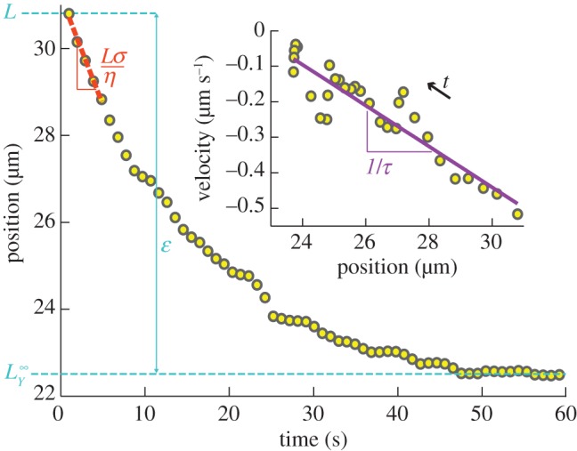
Model-independent measurement of strain , stress-to-viscosity ratio and relaxation time τ. The wound margin position (ellipse semi-axis) is plotted versus time after severing; data from figure 1b–d, see electronic supplementary material, movie S3, along the y-axis. The difference between the initial (L) and final () positions (blue dashed lines) directly yields the value of 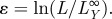The initial velocity (slope of the orange dashed line) yields an estimate of . Inset: velocity, estimated by finite differences of successive positions, versus the position during the first 30 s. An arrow indicates the direction of increasing time t. The slope of a linear fit (purple line) yields the inverse of the relaxation time, (see equation (3.2)).

Our protocol offers several advantages. (i) The experiment directly yields measurements averaged over the severed tissue domain, comprising typically a hundred cells. As discussed below, the domain size is thus an adequate mesoscopic scale, crossing over from detailed cell-level to tissue-level continuous descriptions [6,13]. (ii) The comparison between the initial and final states yields a direct measurement of the strain which existed before severing. (iii) Several cell–cell junctions in various directions are severed at once (rather than step by step) and in the same pupa. Hence one experiment yields a direct measurement of all stress-to-viscosity ratio tensor components. It takes only a few tens of seconds, the typical value of the relaxation time. (iv) Last, but not least, by isolating in time and space an epithelium domain from its neighbouring cells, we can obtain a complete set of well-defined initial, boundary and final conditions for a spatio-temporal model of the retracting domain. We can thus introduce a continuous model, in the spirit of Mayer et al. [30] and taking into account a coupling between space and time dependencies. As explained below, fitting such a model to the displacements in the domain bulk tests the continuous description, suggests an interpretation of the relaxation time and probes the competition between internal viscosity and external friction.

3. Results

3.1. Model-independent measurement of strain, stress-to-viscosity ratio and relaxation time

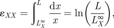
Severing the epithelium reveals the displacement that the epithelium would spontaneously undergo if it were free. We measure the strain using a logarithmic definition [32,37,38], Hencky's ‘true strain’ [39]:

3.1

where L is the initial radius and is the ellipse semi-axis at the end of the relaxation. Similarly 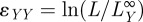. The advantages of this definition are that [32,33]: it is valid at all amplitudes; it is adapted for tensorial measurements; and, finally, it increases the range of validity of the linear elasticity approximation, which applies here even to the highest strain value we measure, 0.45.

Each severing was followed by a relaxation to a final domain strictly smaller than the initial disc (figure 1d), indicating that, before the severing, the tissue had a positive strain in all directions. Since the midline is a symmetry axis, we expected that the strain axes are parallel and perpendicular to it. We checked that this is the case for the fitted ellipse axes, and that, accordingly, the shear strain is indistinguishable from 0. We thus plot and (figure 3a), obtained with absolute precision better than 10⁻². The values are clustered according to the three pupa age groups: is low and isotropic at young age (green cluster), moderate and isotropic at middle age (red), high and anisotropic 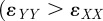) at old age (blue).

Figure 3.

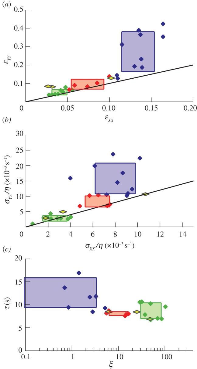
Mechanical state and material properties. Colour code according to pupa development ages: green, young; red, middle-aged; blue, old. The edges of the rectangular regions represent the mean values ± standard deviations for each group. The experiments in the scutum are in yellow. (a) Strain anisotropy: versus . Note the difference in horizontal and vertical scales; the solid line is the first bisectrix y = x, indicating the reference for isotropy. (b) Same for the severed stress-to-viscosity ratio . (c) Relaxation time τ and dimensionless friction-to-viscosity ratio ξ; values are the averages of the measurements along the x- and y-axes (see electronic supplementary material, figure S3). Note the semi-log scale. The blue rectangle takes into account two very small values of ξ, of order 10⁻³ and 10⁻⁴ (below the plotted range).

Similarly, in each experiment, the initial retraction of the wound margins (figure 1c) indicates the sign of the stress: before the severing the tissue was under tensile stress in all directions. This is reminiscent of positive cell junction tensions observed in the wing [25] and in the notum [29]. The initial retraction velocity divided by L yields the stress-to-viscosity ratio (figure 2), in a way which is likely to be independent of any tissue rheological model, as suggested by the following argument. When ablating a single cell–cell junction, force balance shows that the force F exerted by the ablated junction on the neighbouring vertex is proportional to the initial recoil velocity : , where is a friction coefficient [19]. Coarse-graining this relation, and assuming that the main source of dissipation is identical in our experiments which sever many junctions at once, yields , where the factor L is introduced by dimensional analysis. Results for the stress-to-viscosity ratio (figure 3b) are similar to those for : its amplitude and anisotropy are initially small and increase with age; the values are clustered according to the three age groups; no shear stress is detected. Values of span almost two decades, reflecting the sensitivity and precision of the method.

The relaxation time, τ, is obtained from the time evolution of the ellipse axes. Instead of fitting an exponential to the data, we plot the velocity against the position (inset of figure 2). This method is robust and independent of any assumption. A linear regression of the velocity as a function of position yields a slope of , as seen, for example, in the equation

3.2

We find that the relaxation time is approximately isotropic (see electronic supplementary material, figure S3a) and use as an estimate of τ. It is close to 10 s and only slightly varies with the pupa age group (figure 3c, vertical axis).

3.2. Space–time model and measurement of the friction-to-viscosity ratio

To describe the bulk of the retracting domain, we tracked the displacements of around a hundred features in a band of tissue (figure 4 and §5). Spatially averaging their positions by binning them into eight equal-size bins improves the signal-to-noise ratio. We obtain the initial velocity profile versus position (figure 5). For old pupae, it is spatially linear; for middle-aged pupae, it is spatially nonlinear; in the young pupae, immediately after severing only the boundaries move significantly.

Figure 4.

Tracking of feature positions. (a) Positions of features (blue squares), old pupa, data of figure 1c after image denoising. The logarithms of intensity levels are represented in grey scale, and contrast is inverted for clarity. (b) Tracking for the first 30 s (time colour-coded from blue to red), inside a rectangle along the y-axis. (c) Same for the x-axis.

Figure 5.

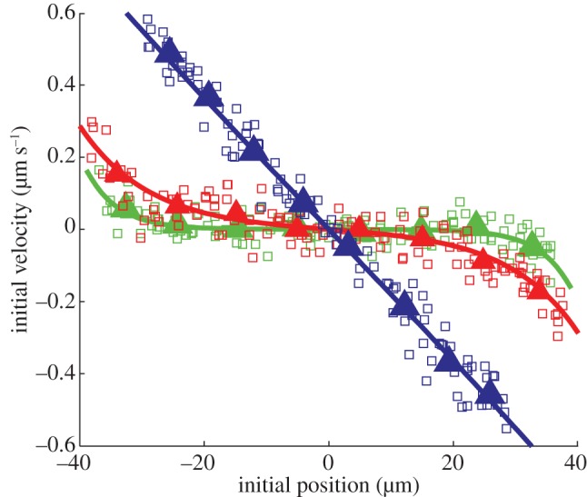
Model-dependent measurement of the friction-to-viscosity ratio ξ. Initial velocity profiles immediately after severing are plotted versus initial position prior to severing, for three typical pupae: young (green), middle-aged (red) and old (blue). Open squares: features, from figure 4b. Closed triangles: same, spatially averaged in eight bins. Lines: fit by a sinh function (equation (3.6)), yielding for ξ a value above, in, or below the measurable range: (green), 5 (red), (blue), respectively.

To account for these observations, we formulate a spatio-temporal, visco-elastic, Kelvin–Voigt model in one dimension of space, where the coordinate z denotes either x or y, and t denotes time after severing (see the electronic supplementary material). Thanks to the definition (3.1), the strain is related without approximation to the velocity v(z, t) through

3.3

We model the effect of friction of the epithelium against the haemolymph and the cuticle as an external fluid friction with coefficient . We find that, when internal viscosity dominates, the strain remains uniform and all parts of the tissue relax exponentially with the same visco-elastic relaxation time , where E is the Young modulus (see electronic supplementary material, figure S4a). When external friction dominates, strain diffuses from the boundaries with a diffusion coefficient and remains thus inhomogeneous at times t smaller than 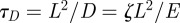(see electronic supplementary material, figure S4b). In the general case, the dynamical equation for the strain field reads

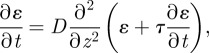3.4

with the conditions 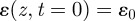initially, at boundaries and at the end. The relative importance of external friction versus internal viscosity is quantified by the dimensionless parameter

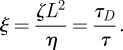3.5

Solving equation (3.4) at short time and integrating over space equation (3.3) at t = 0 yields the initial velocity profile

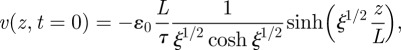3.6

whose curvature is controlled by ξ. We thus estimate ξ by fitting a hyperbolic sine to experimental initial velocity profiles (figure 5). As for the relaxation time, we check that the values and determined in the directions x and y are roughly consistent (see electronic supplementary material, figure S3b): we thus use as an estimate of ξ.

We find that ξ varies more than τ (figure 3c, horizontal axis). The middle-aged group is characterized by intermediate values of ξ (figure 5, red), of the order of 10. According to equation (3.5), this indicates a possible effect of the external friction on the relaxation for scales larger than µm. For both other age groups, the values of ξ should be considered as bounds on the order of magnitude. For old pupae, we find ξ smaller than a few times unity (figure 5, blue). For young pupae, we find ξ larger than a few tens or one hundred (figure 5, green).

This model depends on three parameters measured independently of each other: the initial strain , the visco-elastic time τ and the friction-to-viscosity ratio ξ. To validate the model, we use it to numerically compute the whole space–time map of strains and displacements. We simulate each experiment using the values of τ and ξ measured as described above. Figure 6 shows that we find a good agreement with experimental data. Moreover, we plot the square deviation between experimental and numerical data as a function of the parameter values (see §5). We check that the error landscapes we obtain are broadly consistent with our experimental estimates of ξ and τ (see electronic supplementary material, figure S5).

Figure 6.

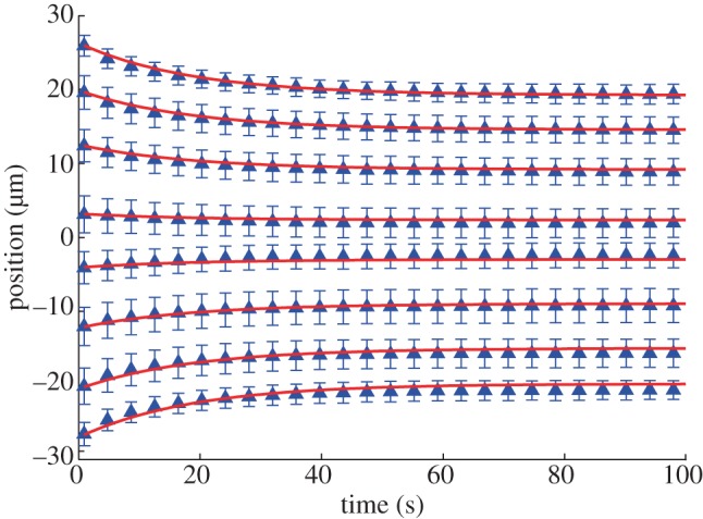
Validation of the model. Blue triangles: positions of features from figure 4b, spatially averaged in bins versus time after severing; bars: standard deviation. Red lines: numerical resolution of equation (3.3), using the measured values , s.

4. Discussion

4.1. Time scale

We report relaxation times τ in the range 5–20 s, and initial velocities in the range 0.1–0.6 µm s⁻¹. This agrees with the values provided by single cell junction ablation: 10–100 s for the relaxation times, 0.1–1 µm s⁻¹ for the initial velocities in other Drosophila tissues [3,25–28]. The model allows τ to be interpreted as a visco-elastic time. Its order of magnitude is typical of the visco-elastic times corresponding to cell internal degrees of freedom [40], also measured in cell aggregates [41,42].

Conversely external degrees of freedom (such as cell–cell rearrangements or cell divisions) would have much larger visco-elastic times: in cell aggregates, they are typically of the order of several hours [11,41,43]. The time scales of morphogenesis in this tissue are also of the order of hours [29], as observed in other tissues as well, such as the Drosophila pupal wing [12]. Indeed continuous models of morphogenetic processes presuppose the existence of such a separation of time scales.

The present experimental data are well described assuming that a single visco-elastic time is relevant. Other experiments display a wide distribution of viscoelastic times [3,28]: the model can easily be modified so as to take this feature into account. Note that, in the presence of friction, the model already predicts that different parts of the severed domain relax at different rates (see electronic supplementary material, figure S4b).

4.2. Length scale

Measurements of , , τ and ξ are performed as averages over the severed disc. The requirements on the averaging scale are that it should be (i) large enough to obtain a sufficient signal-to-noise ratio yielding significant results and (ii) small enough to be able to focus simultaneously on the whole severed ring despite the epithelium surface curvature which is observed in old pupae. The symmetry with respect to the midline observed in figures 1b–d, 5 and 6 acts as a control of the signal-to-noise ratio. The experimentally available range of scales corresponds to 60–100 cell areas; in other words, the semi-axis length L corresponds to 4–5 cell diameters. For old pupae, scales smaller than L are also probed, corresponding to the scale of bins (at least L/2 or L/4, see figures 5 and 6).

4.3. Friction

We experimentally determined the order of magnitude of the dimensionless friction-to-viscosity ratio, ξ (figure 3c, horizontal axis). Obtaining more precise values of ξ would depend on model ingredients, such as depth of ablation along the apico-basal axis, detailed cell geometry, tissue compressibility or type of friction.

For simplicity, we have modelled by a fluid friction [30] the dissipation on either surface of the epithelium, namely the haemolymph at the basal side and the cuticle at the apical side. We do not observe any threshold effect owing to solid friction, and the agreement between model and data justifies a posteriori our assumption.

For young pupae, the initial velocity field is not significantly higher than the noise level (figure 5, green). In this age group, it cannot be used to validate the model, and the estimate of ξ strongly depends on the motion of domain parts located close to the boundary (equation (3.6)).

4.4. Continuous description

In the dorsal thorax, the severed domain fulfills the theoretical requirements for a continuous description: it contains a number of cells much larger than one (large enough to allow for averaging), while being much smaller than the total number of cells in the whole tissue.

One could ask whether averages at scale L are meaningful, owing to variation of cell properties from cell to cell. We speculate that, if heterogeneities within the domain dominated the average, the domain boundary could, in principle, adopt any arbitrary shape compatible with the symmetry. However, in practice, we observed that the domain boundary at the beginning, as well as at the end, of the relaxation also displayed a symmetry (see figure 1b–d and electronic supplementary material, movies S1–S3) and can be fitted by an ellipse: this is consistent with the measurements of and as tensors averaged over scale L.

4.5. Model

Limits of our model lie in its simplifications: one-dimensional treatment, linear elasticity and viscosity, isotropy and homogeneity of material parameters including friction, identical properties of all cells contained in the severed region. However, the agreement between model and experiment is already good and validates these approximations a posteriori. We emphasize that one major goal of this model was to provide an order of magnitude of the friction-to-viscosity ratio ξ. We do not claim that this model is unique, nor that it is general. In the future, we hope to further test the model ingredients and relevance on this epithelium and other quasi-planar ones.

Since its ingredients are general, we expect our model to be of broad relevance when studying the relaxation of quasi-planar epithelia over similar time and length scales. However, the simplifications involved deserve further comments. In fact, completely different hypotheses could also be invoked to explain the spatial nonlinearity in the velocity profile observed for young and middle-aged pupae. For instance, the viscous component of biological tissues could be a nonlinear function of time, strain and strain rate [6]. A strain-dependent viscosity coefficient may lead to a nonlinear velocity profile without the need to invoke any external friction. Alternatively, a spatially heterogeneous friction might also explain the observed velocity profiles. Since a linear velocity profile is observed in older pupae, the amplitude of these additional, more complex ingredients would have to decrease strongly during development.

We believe that our model has the merit of simplicity. It successfully accounts for the description of the velocity profiles at any time. Each of its hypotheses could be tested experimentally and, if experimental results require it, hypotheses could be relaxed to lead to more detailed explorations. We expect that additional ingredients could strongly affect the value of ξ, but that other measurements presented here (namely , and τ) should be robust. The model thus provides a flexible and robust route to a mechanical description of quasi-planar epithelia.

4.6. Perspectives

Building upon classical single-junction laser ablations, our experiments enable measurement of the time evolution of the mechanical state (strain and stress-to-viscosity ratio) and material properties (relaxation time and friction-to-viscosity ratio) during pupa metamorphosis, as well as their anisotropy. This provides relevant ingredients for the modelling of a tissue as a continuous, linear, visco-elastic material.

Moreover, our approach provides a method to explore the biological causality of the observed properties, by analysing mutant phenotypes or by micro-injecting drugs. We conjecture that τ would be affected by low doses of drugs known to modify cytoskeletal rheology such as cytochalasin D [44], CK-666 [45] and Y-27632 [46], which, respectively, inhibit actin polymerization, Arp2/3 complex activity and Rho-kinase activity. We anticipate that modulating cell–cell adhesion by knock-down of E-cadherin or catenins [47] could affect the viscosity. Although we cannot modulate the cell–cuticle adhesion, we could tune cell–matrix adhesion by knock-down of integrin or its linker to the cytoskeleton [47] to affect the friction and thereby modify ξ.

In principle, by establishing a complete map of σ at different positions, one could determine the length scale at which σ varies within the tissue, and check a posteriori whether it is larger than the scale L used to measure σ. However, the present experiments measure the stress up to a dissipative prefactor, the tissue viscosity. Similarly, single cell junction ablation experiments measure force up to a prefactor (a friction coefficient), rarely discussed or measured in the literature. To separate the stress and viscosity variations, alternative methods to directly measure forces and viscosities in live epithelia are thus called for. These include the measurement of cell junction tensions from movie observations [48], where the unknown prefactor, namely the average tension over the whole image, is by definition the same for all junctions. External mechanical manipulation [16–18] yields direct determination of out-of-plane elastic and/or viscous moduli, but the in-plane moduli are only indirectly determined. Another possible strategy could rely on microrheology [49–51]: either passive, by tracking the Brownian diffusion of beads within the cells, or active, by moving (magnetically or optically) a bead back and forth within a cell at a specified frequency. Such measurements could yield a direct access to the value of η, but at the intracellular level. Measuring η at the scale of several cells directly, or indirectly by measuring E and τ and using the relation , could be possible, but we are not aware yet of a published method.

Since is a dimensionless geometrical quantity, its value is insensitive to cell size: the observed approximately sevenfold increase in cannot be related to changes in cell size over time. It should involve other causes, which remain to be determined. Part of the measured increase in values may be due to cell divisions, which decrease the average cell area by a factor of approximately 2 between young and old pupae. The observed increase is a factor of approximately 25, and thus should involve other causes as well. One candidate is a decrease of the tissue viscosity η. However, the near constancy of the visco-elastic time would then imply a corresponding increase in tissue elasticity, a rather unlikely coincidence. We therefore expect that stronger tensile forces are at work in the tissue in older pupae. From 18 h after pupa formation onwards, the lateral part of the scutellum undergoes apical cell contractions that shape the lateral domain of the tissue [29]. This observation led us to divide the ablation experiments into the three age groups. It may also explain the changes in mechanical properties measured in the tissue for middle-aged and old pupae. To precisely analyse the causes of the increases in and would therefore require identification of the genes that specifically affect the lateral contraction of the tissue.

Our experimental method should be applicable to other tissues. Performing experiments in an epithelium which is flat enough to significantly increase L, and with a sufficient signal-to-noise ratio on the estimate of ξ, would enable the scaling of ξ versus L given by equation (3.5) to be checked.

5. Methods

5.1. Experiments

Drosophila melanogaster larvae were collected at the beginning of metamorphosis (pupa formation) [52]. The pupae were kept at 25°C, then dissected and mounted as described in Ségalen et al. [53] (see electronic supplementary material, figure S1). Using the adherens junction protein E-cadherin fused to green fluorescent protein [54], we imaged the apical cell junctions by fluorescent microscopy [53].

The time-lapse laser-scanning microscope LSM710 NLO (Carl Zeiss MicroImaging) collected 512 × 512 pixel images in mono-photon mode at 488 nm excitation (pixel size in the range 0.24–0.29 µm) through a Plan-Apochromat 63 × 1.40 oil objective. Before and after severing, the time interval between two consecutive frames was either 393 or 970 ms according to the scanning mode (bi- or mono-directional), without any apparent effect on the results presented here. We focused on the adherens junctions to be severed; owing to the epithelial surface curvature especially in old pupae, adherens junctions of innermost and outermost regions were slightly out of focus (see figure 1 and electronic supplementary material, movies S1–S3).

We defined a region of interest as an annular region between two concentric circles. We severed it at the 10th frame (figure 1) and defined L as the radius of its inner circle. Laser severing was performed using Ti:sapphire laser (Mai Tai DeepSee, Spectra Physics) in two-photon mode at 890 nm, less than 100 fs pulses, 80 MHz repetition rate, ∼0.2 W at the back focal plane, used at slightly less than full power to avoid cavitation (see electronic supplementary material, figure S2) [21]. Severing itself had a duration ranging from 217 to 1300 ms (according to the size of the region of interest and the scanning mode) during which no image was acquired. We could check that the severing had been effective in removing the adherens junctions, rather than simply bleaching them (see electronic supplementary material, figure S2): after retraction, the cells at the wound margin moved apart more than a cell diameter; moreover, there was no fluorescence recovery (figure 1d).

5.2. Analysis

At the tissue scale, for each frame after the severing, the inner severed tissue boundary was fitted with an ellipse (figure 1c,d) using the ovuscule ImageJ plugin [35]. We have modified it so that each fitting procedure started from the ellipse fitted on the preceding image: such tracking improved the speed and robustness. Data of figure 2 are linearly fitted over a five-frame sliding window in order to improve the signal-to-noise ratio of position and velocity determinations.

Independently, at the cell scale, images were denoised with Safir software [55,56]. We took the logarithm of the grey levels, to obtain comparable intensity gradients in differently contrasted parts of the image (figure 4a). This allowed us to use the Kanade–Lucas–Tomasi (KLT) [57,58] tracking algorithm [59] by selecting approximately 10² ‘features’ of interest, corresponding to most cell vertices (figure 4a). Features were tracked from frame to frame: they followed the cell vertex movement towards the centre, and we have observed no cell neighbour swapping. We checked that the features' centre of mass had only a small displacement, which we subtracted from individual feature displacements without loss of generality. To implement a quasi-one-dimensional analysis, we collected the features in a band along the y-axis and similarly along the x-axis (figure 4b,c), and both axes were analysed separately. The band width (here 1/3 of the initial circle diameter) was chosen to be large enough to perform large statistics on features, and small enough to treat the features' displacement as one-dimensional.

5.3. Comparison of model with experimental data

We numerically solved adimensionalized equations (see the electronic supplementary material) using the Matlab solver pdepde. For a given set of parameter values , we calculated from the strain of the feature of largest initial amplitude, and rescaled the solution of electronic supplementary material, equation 14, so as to satisfy electronic supplementary material, equation 3. Using the experimental initial positions of features and the calculated strain field , we simulated the trajectories , , where was the number of features.

The mismatch ℰ with our computation was evaluated by comparison with the experimental trajectories, ,

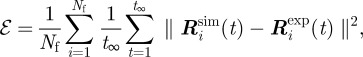5.1

where denoted the Euclidean norm, and the number of movie images.

References

- 1.Lecuit T., Lenne P. F. 2007. Cell surface mechanics and the control of cell shape, tissue patterns and morphogenesis. Nat. Rev. Mol. Cell Biol. 8, 633–644 10.1038/nrm2222 (doi:10.1038/nrm2222) [DOI] [PubMed] [Google Scholar]
- 2.Chen C. S., Tan J., Tien J. 2004. Mechanotransduction at cell-matrix and cell-cell contacts. Annu. Rev. Biomed. Eng. 6, 275–302 10.1146/annurev.bioeng.6.040803.140040 (doi:10.1146/annurev.bioeng.6.040803.140040) [DOI] [PubMed] [Google Scholar]
- 3.Ma X., Lynch H. E., Scully P. C., Hutson M. S. 2009. Probing embryonic tissue mechanics with laser hole drilling. Phys. Biol. 6, 036004 10.1088/1478-3975/6/3/036004 (doi:10.1088/1478-3975/6/3/036004) [DOI] [PubMed] [Google Scholar]
- 4.Lecuit T., Le Goff L. 2007. Orchestrating size and shape during morphogenesis. Nature 450, 189–192 10.1038/nature06304 (doi:10.1038/nature06304) [DOI] [PubMed] [Google Scholar]
- 5.Mammoto T., Ingber D. E. 2010. Mechanical control of tissue and organ development. Development 137, 1407–1420 10.1242/dev.024166 (doi:10.1242/dev.024166) [DOI] [PMC free article] [PubMed] [Google Scholar]
- 6.Fung Y. C. 1993. Biomechanics: mechanical properties of living tissues. Berlin, Germany: Springer [Google Scholar]
- 7.Hufnagel L., Teleman A. A., Rouault H., Cohen S. M., Shraiman B. I. 2007. On the mechanism of wing size determination in fly development. Proc. Natl Acad Sci. USA 104, 3835–3840 10.1073/pnas.0607134104 (doi:10.1073/pnas.0607134104) [DOI] [PMC free article] [PubMed] [Google Scholar]
- 8.Bittig T., Wartlick O., Kicheva A., Gonzalez-Gaitan M., Jülicher F. 2008. Dynamics of anisotropic tissue growth. New J. Phys. 10, 063001 10.1088/1367-2630/10/6/063001 (doi:10.1088/1367-2630/10/6/063001) [DOI] [Google Scholar]
- 9.Blanchard G. B., Kabla A. J., Schultz N. L., Butler L. C., Sanson B., Gorfinkiel N., Mahadevan L., Adams R. J. 2009. Tissue tectonics: morphogenetic strain rates, cell shape change and intercalation. Nat. Method 6, 458–464 10.1038/nmeth.1327 (doi:10.1038/nmeth.1327) [DOI] [PMC free article] [PubMed] [Google Scholar]
- 10.Butler L. C., Blanchard G. B., Kabla A. J., Lawrence N. J., Welchman D. P., Mahadevan L., Adams R. J., Sanson B. 2009. Cell shape changes indicate a role for extrinsic tensile forces in Drosophila germ-band extension. Nat. Cell Biol. 11, 859–864 10.1038/ncb1894 (doi:10.1038/ncb1894) [DOI] [PubMed] [Google Scholar]
- 11.Ranft J., Basan M., Elgeti J., Joanny J.-F., Prost J., Jülicher F. 2010. Fluidization of tissues by cell division and apoptosis. Proc. Natl Acad Sci. USA 107, 20 863–20 868 10.1073/pnas.1011086107 (doi:10.1073/pnas.1011086107) [DOI] [PMC free article] [PubMed] [Google Scholar]
- 12.Aigouy B. et al. 2010. Cell flow reorients the axis of planar polarity in the wing epithelium of Drosophila. Cell 142, 773–786 10.1016/j.cell.2010.07.042 (doi:10.1016/j.cell.2010.07.042) [DOI] [PubMed] [Google Scholar]
- 13.Batchelor G. K. 2000. An introduction to fluid dynamics. Cambridge, UK: Cambridge University Press [Google Scholar]
- 14.Ophir J., Cespedes I., Garra B., Ponnekanti H., Huang Y., Maklad N., 1996. Elastography: ultrasonic imaging of tissue strain and elastic modulus in vivo. Eur. J. Ultrasound 3, 49–70 10.1016/0929-8266(95)00134-4 (doi:10.1016/0929-8266(95)00134-4) [DOI] [Google Scholar]
- 15.Nienhaus U., Aegerter-Wilmsen T., Aegerter C. M. 2009. Determination of mechanical stress distribution in Drosophila wing discs using photoelasticity. Mech. Dev. 126, 942–949 10.1016/j.mod.2009.09.002 (doi:10.1016/j.mod.2009.09.002) [DOI] [PubMed] [Google Scholar]
- 16.Desprat N., Supatto W., Pouille P., Beaurepaire E., Farge E. 2008. Tissue deformation modulates twist expression to determine anterior midgut differentiation in Drosophila embryos. Dev. Cell 15, 470–477 10.1016/j.devcel.2008.07.009 (doi:10.1016/j.devcel.2008.07.009) [DOI] [PubMed] [Google Scholar]
- 17.Fleury V., et al. 2010. Introducing the scanning air puff tonometer for biological studies. Phys. Rev. E 81, 021920. 10.1103/PhysRevE.81.021920 (doi:10.1103/PhysRevE.81.021920) [DOI] [PubMed] [Google Scholar]
- 18.Peaucelle A., Braybrook S., Le Guillou L., Bron E., Kuhlemeier C., Höfte H. 2011. Pectin-induced changes in cell wall mechanics underlie organ initiation in Arabidopsis. Curr. Biol. 21, 1720–1726 10.1016/j.cub.2011.08.057 (doi:10.1016/j.cub.2011.08.057) [DOI] [PubMed] [Google Scholar]
- 19.Rauzi M., Lenne P. F. 2011. Cortical forces in cell shape changes and tissue morphogenesis. Curr. Top. Dev. Biol. 95, 93–144 10.1016/B978-0-12-385065-2.00004-9 (doi:10.1016/B978-0-12-385065-2.00004-9) [DOI] [PubMed] [Google Scholar]
- 20.Hutson M. S., Tokutake Y., Chang M.-S., Bloor J. W., Venakides S., Kiehart D. P., Edwards G. S. 2003. Forces for morphogenesis investigated with laser microsurgery and quantitative modeling. Science 300, 145–149 10.1126/science.1079552 (doi:10.1126/science.1079552) [DOI] [PubMed] [Google Scholar]
- 21.Hutson M. S., Ma X. 2007. Plasma and cavitation dynamics during pulsed laser microsurgery in vivo. Phys. Rev. Lett. 99, 158104. 10.1103/PhysRevLett.99.158104 (doi:10.1103/PhysRevLett.99.158104) [DOI] [PubMed] [Google Scholar]
- 22.Hutson M. S., Veldhuis J., Ma X., Lynch H. E., Cranston P. G., Brodland G. W. 2009. Combining laser microsurgery and finite element modeling to assess cell-level epithelial mechanics. Biophys. J. 97, 3075–3085 10.1016/j.bpj.2009.09.034 (doi:10.1016/j.bpj.2009.09.034) [DOI] [PMC free article] [PubMed] [Google Scholar]
- 23.Kiehart D. P., Galbraith C. G., Edwards K. A., Rickoll W. L., Montague R. A. 2000. Multiple forces contribute to cell sheet morphogenesis for dorsal closure in Drosophila development. J. Cell Biol. 149, 471–490 10.1083/jcb.149.2.471 (doi:10.1083/jcb.149.2.471) [DOI] [PMC free article] [PubMed] [Google Scholar]
- 24.Peralta X. G., Toyama Y., Hutson M. S., Montague R., Venakides S., Kiehart D. P., Edwards G. S. 2007. Upregulation of forces and morphogenic asymmetries in dorsal closure during Drosophila development. Biophys. J. 92, 2583–2596 10.1529/biophysj.106.094110 (doi:10.1529/biophysj.106.094110) [DOI] [PMC free article] [PubMed] [Google Scholar]
- 25.Farhadifar R., Röper J., Aigouy B., Eaton S., Jülicher F. 2007. The influence of cell mechanics, cell-cell interactions, and proliferation on epithelial packing. Curr. Biol. 17, 2095–2104 10.1016/j.cub.2007.11.049 (doi:10.1016/j.cub.2007.11.049) [DOI] [PubMed] [Google Scholar]
- 26.Rauzi M., Verant P., Lecuit T., Lenne P. F. 2008. Nature and anisotropy of cortical forces orienting Drosophila tissue morphogenesis. Nat. Cell. Biol. 10, 1401–1410 10.1038/ncb1798 (doi:10.1038/ncb1798) [DOI] [PubMed] [Google Scholar]
- 27.Landsberg K. P., Farhadifar R., Ranft J., Umetsu D., Widmann T. J., Bittig T., Said A., Jülicher F., Dahmann C. 2009. Increased cell bond tension governs cell sorting at the Drosophila anteroposterior compartment boundary. Curr. Biol. 19, 1950–1955 10.1016/j.cub.2009.10.021 (doi:10.1016/j.cub.2009.10.021) [DOI] [PubMed] [Google Scholar]
- 28.Fernandez-Gonzalez R., Simoes Sd. M., Röper J., Eaton S., Zallen J. A. 2009. Myosin II dynamics are regulated by tension in intercalating cells. Dev. Cell 17, 736–743 10.1016/j.devcel.2009.09.003 (doi:10.1016/j.devcel.2009.09.003) [DOI] [PMC free article] [PubMed] [Google Scholar]
- 29.Bosveld F., et al. 2012. Mechanical control of morphogenesis by Fat/Dachsous/Four-Jointed planar cell polarity pathway. Science 336, 724–727 10.1126/science.1221071 (doi:10.1126/science.1221071) [DOI] [PubMed] [Google Scholar]
- 30.Mayer M., Depken M., Bois J. S., Jülicher F., Grill S. W. 2010. Anisotropies in cortical tension reveal the physical basis of polarizing cortical flows. Nature 467, 617–621 10.1038/nature09376 (doi:10.1038/nature09376) [DOI] [PubMed] [Google Scholar]
- 31.Martin A. C., Gelbart M., Fernandez-Gonzalez R., Kaschube M., Wieschaus E. F. 2010. Integration of contractile forces during tissue invagination. J. Cell Biol. 188, 735–749 10.1083/jcb.200910099 (doi:10.1083/jcb.200910099) [DOI] [PMC free article] [PubMed] [Google Scholar]
- 32.Janiaud E., Graner F. 2005. Foam in a two-dimensional Couette shear: a local measurement of bubble deformation. J. Fluid Mech. 532, 243–267 10.1017/S0022112005004052 (doi:10.1017/S0022112005004052) [DOI] [Google Scholar]
- 33.Graner F., Dollet B., Raufaste C., Marmottant P. 2008. Discrete rearranging disordered patterns, part I: robust statistical tools in two or three dimensions. Eur. Phys. J. E. 25, 349–369 10.1140/epje/i2007-10298-8 (doi:10.1140/epje/i2007-10298-8) [DOI] [PubMed] [Google Scholar]
- 34.Bainbridge S. P., Bownes M. 1981. Staging the metamorphosis of Drosophila melanogaster. J. Embryol. Exp. Morph. 66, 57–80 [PubMed] [Google Scholar]
- 35.Thévenaz P., Delgado-Gonzalo R., Unser M. 2011. The ovuscule. IEEE Trans. Pattern Anal. Mach. Intell. 33, 382–393 10.1109/TPAMI.2010.112 (doi:10.1109/TPAMI.2010.112) [DOI] [PubMed] [Google Scholar]
- 36.Langevin J. et al. 2005. Drosophila exocyst components sec5, sec6, and sec15 regulate DE-Cadherin trafficking from recycling endosomes to the plasma membrane. Dev. Cell 9, 365–376 10.1016/j.devcel.2005.07.013 (doi:10.1016/j.devcel.2005.07.013) [DOI] [PubMed] [Google Scholar]
- 37.Hoger A. 1987. The stress conjugate to logarithmic strain. Int. J. Solids Struct. 23, 1645–1656 10.1016/0020-7683(87)90115-6 (doi:10.1016/0020-7683(87)90115-6) [DOI] [Google Scholar]
- 38.Farahani K., Naghdabadi R. 2000. Conjugate stresses of the Seth-Hill strain tensors. Int. J. Solids Struct. 37, 5247–5255 10.1016/S0020-7683(99)00209-7 (doi:10.1016/S0020-7683(99)00209-7) [DOI] [Google Scholar]
- 39.Tanner R., Tanner E. 2003. Heinrich Hencky: a rheological pioneer. Rheol. Acta 42, 93–101 10.1007/s00397-002-0259-6 (doi:10.1007/s00397-002-0259-6) [DOI] [Google Scholar]
- 40.Wottawah F., Schinkinger S., Lincoln B., Ananthakrishnan R., Romeyke M., Guck J., Käs J. 2005. Optical rheology of biological cells. Phys. Rev. Lett. 94, 098103. 10.1103/PhysRevLett.94.098103 (doi:10.1103/PhysRevLett.94.098103) [DOI] [PubMed] [Google Scholar]
- 41.Marmottant P., et al. 2009. The role of fluctuations and stress on the effective viscosity of cell aggregates. Proc. Natl Acad Sci. USA 106, 17 271–17 275 10.1073/pnas.0902085106 (doi:10.1073/pnas.0902085106) [DOI] [PMC free article] [PubMed] [Google Scholar]
- 42.Guevorkian K., Gonzalez-Rodriguez D., Carlier C., Dufour S., Brochard-Wyart F. 2011. Mechanosensitive shivering of model tissues under controlled aspiration. Proc. Natl Acad Sci. USA 108, 13 387–13 392 10.1073/pnas.1105741108 (doi:10.1073/pnas.1105741108) [DOI] [PMC free article] [PubMed] [Google Scholar]
- 43.Guevorkian K., Colbert M., Durth M., Dufour S., Brochard-Wyart F. 2010. Aspiration of biological viscoelastic drops. Phys. Rev. Lett. 104, 218101. 10.1103/PhysRevLett.104.218101 (doi:10.1103/PhysRevLett.104.218101) [DOI] [PubMed] [Google Scholar]
- 44.Flanagan M. D., Lin S. 1980. Cytochalasins block actin filament elongation by binding to high affinity sites associated with F-actin. J. Biol. Chem. 255, 835–838 [PubMed] [Google Scholar]
- 45.Nolen B. J., Tomasevic N., Russell A., Pierce D. W., Jia Z., McCormick C. D., Hartman J., Sakowicz R., Pollard T. D. 2009. Characterization of two classes of small molecule inhibitors of Arp2/3 complex. Nature 460, 1031–1034 10.1038/nature08231 (doi:10.1038/nature08231) [DOI] [PMC free article] [PubMed] [Google Scholar]
- 46.Uehata M., et al. 1997. Calcium sensitization of smooth muscle mediated by a Rho-associated protein kinase in hypertension. Nature 389, 990–994 10.1038/40187 (doi:10.1038/40187) [DOI] [PubMed] [Google Scholar]
- 47.Papusheva E., Heisenberg C. P. 2010. Spatial organization of adhesion: force-dependent regulation and function in tissue morphogenesis. EMBO J. 29, 2753–2768 10.1038/emboj.2010.182 (doi:10.1038/emboj.2010.182) [DOI] [PMC free article] [PubMed] [Google Scholar]
- 48.Brodland G. W. et al. 2010. Video force microscopy reveals the mechanics of ventral furrow invagination in Drosophila. Proc. Natl Acad Sci. USA 107, 22 111–22 116 10.1073/pnas.1006591107 (doi:10.1073/pnas.1006591107) [DOI] [PMC free article] [PubMed] [Google Scholar]
- 49.MacKintosh F., Schmidt C. 1999. Microrheology. Curr. Opinion Coll. Interface Sci. 4, 300–307 [Google Scholar]
- 50.Panorchan P., Lee J. S. H., Daniels B. R., Kole T. P., Tseng Y., Wirtz D. 2007. Probing cellular mechanical responses to stimuli using ballistic intracellular nanorheology. Methods Cell Biol. 83, 115–140 10.1016/S0091-679X(07)83006-8 (doi:10.1016/S0091-679X(07)83006-8) [DOI] [PubMed] [Google Scholar]
- 51.Crocker J. C., Hoffman B. D. 2007. Multiple-particle tracking and two-point microrheology in cells. Methods Cell Biol. 83, 141–178 10.1016/S0091-679X(07)83007-X (doi:10.1016/S0091-679X(07)83007-X) [DOI] [PubMed] [Google Scholar]
- 52.Roberts D. B. 1998. Drosophila: a practical approach, 2nd edn Oxford, UK: Oxford University Press [Google Scholar]
- 53.Ségalen M., Johnston C. A., Martin C. A., Dumortier J. G., Prehoda K. E., David N. B., Doe C. Q., Bellaïche Y. 2010. The Fz-Dsh planar cell polarity pathway induces oriented cell division via Mud/NuMA in Drosophila and zebrafish. Dev. Cell 19, 740–752 10.1016/j.devcel.2010.10.004 (doi:10.1016/j.devcel.2010.10.004) [DOI] [PMC free article] [PubMed] [Google Scholar]
- 54.Oda H., Tsukita S. 2001. Real-time imaging of cell–cell adherens junctions reveals that Drosophila mesoderm invagination begins with two phases of apical constriction of cells. J. Cell Sci. 114, 493–501 [DOI] [PubMed] [Google Scholar]
- 55.Kervrann C., Boulanger J. 2006. Optimal spatial adaptation for patch-based image denoising. IEEE Trans. Image Process 15, 2866–2878 10.1109/TIP.2006.877529 (doi:10.1109/TIP.2006.877529) [DOI] [PubMed] [Google Scholar]
- 56.Boulanger J., Kervrann C., Bouthemy P., Elbau P., Sibarita J.-B., Salamero J. 2010. Patch-based nonlocal functional for denoising fluorescence microscopy image sequences. IEEE Trans. Med. Imaging 29, 442–454 10.1109/TMI.2009.2033991 (doi:10.1109/TMI.2009.2033991) [DOI] [PubMed] [Google Scholar]
- 57.Lucas B., Kanade T. 1981. An iterative image registration technique with an application to stereo vision. In Proc. 7th Int. Joint Conf. on Artificial Intelligence, Vancouver, BC, 24–28 August 1981, pp. 121–130 [Google Scholar]
- 58.Tomasi C., Kanade T. 1991. Detection and tracking of point features. Technical Report no. CMU-CS-91-132. Carnegie Mellon University, Pittsburgh, PA [Google Scholar]
- 59.KLT Kanade–Lucas–Tomasi feature tracker. See http://www.ces.clemson.edu/∼stb/klt/ [Google Scholar]