The optimal deployment of synergistic antibiotics: a control-theoretic approach

Abstract

Medical and pharmacological communities have long searched for antimicrobial drugs that increase their effect when used in combination, an interaction known as synergism. These drug combinations, however, impose selective pressures in favour of multi-drug resistance and as a result, the benefit of synergy may be lost after only a few bacterial generations. Furthermore, there is experimental evidence that antibiotic treatment can disrupt colonization resistance by shifting the balance between enteropathogenic and commensal bacteria in favour of the pathogens, with the potential to increase the risk of infections. So, we ask, what is the best way of using synergistic drugs? We pose an evolutionary model of commensal and pathogenic bacteria competing in a continuous culture device for a single limiting carbon source under the effect of two bacteriostatic and synergistic antibiotics. This model allows us to evaluate the efficacy of different drug deployment strategies and, using ideas from optimal control theory, to understand whether there are circumstances in which other types of therapy might be favoured over those based on fixed-dose multi-drug combinations. Our main result can be stated thus: the optimal deployment of synergistic antibiotics to remove a pathogen in the presence of commensal bacteria in our model system occurs not in combination, but by deploying them sequentially.

1. Introduction

The evolution and spread of antibiotic resistance in pathogenic bacteria represent a potentially grave public health problem [1,2]. A common approach to dealing with the evolution of antibiotic resistance and to increase the efficacy of antimicrobial treatments is to use multi-drug combination therapies [3–5]. However, the profiles of interaction between different antibiotics and their long-term effect on drug resistance are still poorly understood. It has even been suggested, for example, that synergistic drug combinations, those usually preferred in clinical settings, may serve to promote the evolution of drug resistance [6–8].

The standard pharmacological approach to therapy design focuses on antibiotic combinations that increase drug efficacy [9] without accounting for the effects drugs might have either on the evolution of drug resistance or on the innate resistance provided by the host's microbiota. And yet it has been shown that the disruption of the gut microbiota that occurs when antimicrobials are prescribed may increase the risk of infection [10,11]. So, as a model to better understand these issues, we undertake a theoretical study of an experimental device (an extension of the basic chemostat) in which two bacterial species compete for a single limiting resource. By deploying antimicrobial agents in different combinations into the device, we aim to use the drugs to remove only one of those species.

To achieve this, we first define a growth inhibition coefficient that characterizes the interaction between both antibiotics at different concentrations, using standard enzymatic assumptions of how drugs inhibit their targets. From the resulting growth inhibition surfaces, we construct an evolutionary model that allows us to study the effect that different drug combinations may have on the heterogeneous population of bacteria cultured in media with a single carbon source. Our experimental design also permits dynamic control of the input of both antibiotics into the device. As explained later, the interaction between the two drugs is assumed throughout to be synergistic, whereby each enhances the other's effect, a property we impose on our mathematical models and validated using a standard experimental system described in appendix D.

Our main results are stated in and beyond §2.8, wherein it is shown that we can use optimization techniques to engineer treatment protocols that support commensal bacteria while minimizing the density of pathogens, even in the direst of possible circumstances. The latter alludes to a biological assumption we engineer into the problem that makes existence as difficult as possible for the commensal species: the pathogen population has at least one phenotype that is fitter than the commensal bacterium in all abiotic environments and at all antibiotic concentrations. We call this complete competitive advantage of the pathogen over the commensal.

2. Results

2.1. Drug interactions and the evolution of resistance

The so-called bacteriostatic antibiotics do not necessarily kill bacteria but suppress their growth by inhibiting DNA replication, RNA synthesis or by interfering with other aspects of cellular function. Although the precise mechanism of action of drugs from different functional classes can be difficult to capture mathematically, in some cases, we can model the inhibition of bacterial growth rate through the competitive inhibition of an essential metabolite. For example, the antibiotic rifampicin inhibits RNA polymerase by binding to its β subunit, erythromycin binds to the 50S ribosomal subunit inhibiting protein synthesis and doxycycline binds to the 30S subunit and inhibits binding of aminoacyl-tRNA to the mRNA-ribosome complex. We use these drugs to motivate our approach.

Assuming the molecular dynamics supporting the small antibiotic molecule and protein target is in statistical equilibrium, competitive inhibition processes like those described earlier can be modelled by kinetic equations. Indeed, using basic enzymatics, dimensionless expressions for inhibition of RNA transcription as a function of the antibiotic rifampicin present in the cell may be derived [12]. So, if A is the concentration of antibiotic within the cell, the reduction in the rate of RNA transcription, γ(A) say, is a number between 0 and 1 of the basic form

2.1

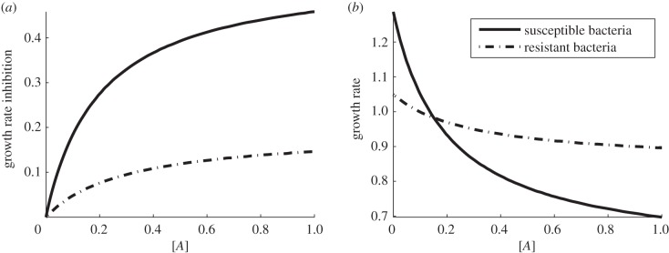
where κ₁ and κ₂ are parameters. They may be considered as evolvable phenotypes of the cell, and the susceptibility of each cell type to the antibiotic can be determined, as illustrated in figure 1a.

Figure 1.

(a) Growth rate inhibition as a function of antibiotic concentration (the dimensionless growth inhibition denoted γ(A) throughout this section). (b) Growth rate (per hour) as a function of antibiotic concentration in the environment with maximum resource available S ≡S₀. Here we see that the antibiotic-resistant phenotype (dashed line) has a higher growth rate than the susceptible strain (solid line) when the antibiotic concentration is high. The fitness cost associated with resistance is expressed by having a lower growth rate when the antibiotic concentration, A, is low.

With rifampicin in mind, let us now assume for simplicity that bacterial growth rate is proportional to the resource uptake rate multiplied by the rate of transcription of RNA; other myriad features of the cell's metabolism are then incorporated into a single parameter, c. We then represent the growth rate, G say, of a cellular phenotype in terms of the concentration of available limiting resource, denoted by S, and the concentration of a bacteriostatic antibiotic present in the environment, A, as follows:

2.2

Throughout, S and A will be functions of time, t, and the constant of proportionality here, c, is a resource conversion or cell efficiency parameter measured in cells per microgram where u(S) is the resource uptake rate. The latter will be a Michaelis–Menten function with affinity for resource, K, and maximum growth rate, V_max, specifically

2.3

Bacterial phenotypes are now defined using growth rates and antibiotic-susceptibility profiles, properties that can be described in terms of the set of phenotypic parameters . For example, if an antibiotic-susceptible bacterial phenotype has growth rate denoted by

then a resistant phenotype would have, by definition, a higher growth rate than antibiotic-susceptible bacteria at high antibiotic concentrations. More formally, this means that if the growth rate of a resistant phenotype is given by the function

then there must exist a critical antibiotic concentration A* > 0 for which for all .

It is well-known [13,14] that antibiotic-resistant phenotypes may encounter a reduction in fitness in an antibiotic-free environment, which is known as fitness cost of resistance. In our modelling framework, this property can be realized by imposing a lower resource uptake rate u^r(S) < u^s(S) and therefore a lower growth rate at low antibiotic concentrations (figure 1b) that results in the property G^r(S,0) < G^s(S,0).

2.2. Antibiotic interactions

Intuitively, antibiotics combinations can be classified as synergistic (if the drugs interact to increase each other's effect), antagonistic (if their combined effect is less than the most effective drug used individually) or additive (if they do not interact). Although this intuitive classification of drug interactions seems straightforward, the difficulty of rigorously defining the null interaction has been a matter of controversy for decades and the subject of a series of misconceptions [15,16].

The most widely accepted test to quantify drug interactions are isobolograms as proposed by Loewe [17] to measure synergy. This experiment measures the in vitro susceptibility of a population of bacteria growing in a bidimensional array of different combinations of antibiotics. Optical densities (ODs) or colony forming units are measured at the end of the experiment and from the dose-response surface so obtained; the interaction can be classified by lines of equal drug effect that are known as isoboles. Here, instead of modelling population-level dose-response surfaces directly, we are going to derive them as an emergent property of a model constructed from single-cell inhibition rates.

In order to describe drug interactions at the cellular level, we are going to assume that at any given moment in time, two antibiotics are present in the environment at concentrations A and B and that the bacterial growth rate can be described by a function, G(S,A,B), that depends on the concentrations of both drugs and upon the concentration of the limiting resource, S, in the environment. Just as in the case of a single drug, this growth function will be modelled as a standard Michaelis–Menten term multiplied by a growth inhibition coefficient γ(A,B) that depends on the concentration of both drugs:

2.4

Again, c denotes a resource conversion rate, and u(S) is the resource uptake function defined in equation (2.3). The function γ(A,B) satisfies γ(A,0) = γ_A(A) and γ(0,B) = γ_B(B), where γ_A(A) and γ_B(B) are growth inhibition functions that characterize the single and separate use of each antibiotic.

We shall represent the density of a population of pathogenic bacteria growing under resource limitation and under the effect of two bacteriostatic antibiotics of concentrations A(t) and B(t) by the time-series P(t). We will then assume that the concentration of bacterium per unit of volume is so high and uniformly distributed in space that it is possible to describe the ecological interactions between different bacterial populations using deterministic models based on the mass action law [18]. The one we use here is stated as follows:

2.5a

2.5b

2.5c

2.5d

with initial conditions x(0) = (S(0),P(0),A(0),B(0)). Constants a and b are phenotypic parameters that denote the rate of binding and the uptake rate of antibiotic molecules to their cellular targets. Throughout, S₀ will represent the maximal concentration of the limiting carbon source.

2.3. Synergistic antibiotics

Let us choose two basal concentrations for each drug, denoting them A₀ and B₀, respectively, and measure them in micrograms per millilitre. We then define the optimal drug ratio θ* where 0 ≤ θ* ≤ 1 to be that proportion, θ, that minimizes the cellular growth inhibition coefficient for θ in [0, 1]:

Any treatment that deploys a fixed combination of drugs at a constant ratio, θ say, will be called a combination treatment in the remainder.

As discussed already, two drugs act synergistically when their combined effect is larger than the effect of each drug when used separately, a property represented formally by θ* being inside the interval (0,1). If the optimal drug combination in the earlier-mentioned sense uses only one of the drugs, that is θ* = 0 or θ* = 1, then we say their interaction is antagonistic. If γ(θA₀, (1 − θ)B₀) is constant as a function of θ and so θ* could be any value between 0 and 1, we then say that either the drugs do not interact with each other, or their interaction is additive; we consider the latter two statements to be synonymous.

We restrict our attention to antibiotic combination therapies that use two bacteriostatic antibiotics from closely related functional classes, namely those that target subunits of the same enzyme complex. We will, however, assume that they bind to non-overlapping sites on that complex. Assuming that we can therefore model their interaction as mutually non-exclusive competitive inhibitors, we provide a rationale in appendix C that allows us to write their combined inhibitory effect in the following functional form:

2.6

where κ_A, κ_B and κ_AB may be constants or rational, bounded functions of (A,B) derived from the kinetics of the drugs and their common target.

When there are multiple types of bacteria present in an evolutionary model, the inhibition of the growth rate of bacterial type i due to the use of a single antibiotic, A say, will be described by the inhibition function

where κ₂ⁱ will be called the antibiotic affinity of the cell and κ₁ⁱ controls the level of maximal growth inhibition. Similarly, the growth inhibition function of antibiotic B in the absence of antibiotic A is given by

We shall also suppose for simplicity that the bacteriostatic effect of combining both antibiotics is determined by the multiplicative effect of the concentrations of each antibiotic by assuming the multi-drug growth inhibition function γ(A,B) to be given by

2.7

We acknowledge that interactions between drugs targeting different enzymes in a pathway do not necessarily lead to such simple functional forms for the drug inhibition surface as that described in (2.7) (see [19], for example). This is why we have restricted our attention to drugs targeting essentially the same enzyme. However, we argue that in some cases, our simple rationale should be able to capture the interaction between two antibiotics that bind to non-overlapping sites of the same target and whose interaction is known to be synergistic, for example the drug pair studied in Hegreness et al. [6].

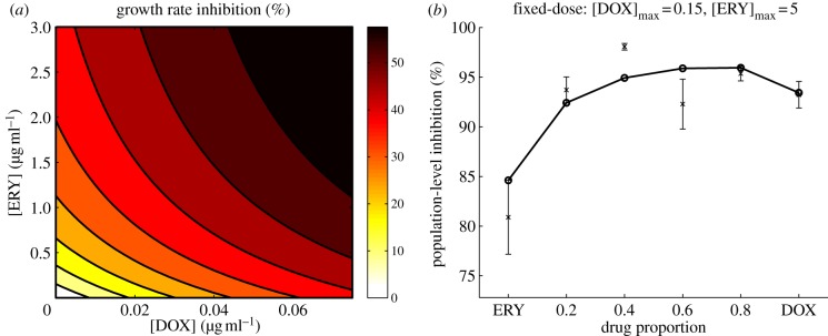
To test this, we measured the inhibitory effect on an isogenic population of bacteria growing under resource limitation and under the effect of two bacteriostatic antibiotics that target different sites in the ribosome, thus inhibiting protein synthesis. These were doxycycline that binds to the 30S subunit and erythromycin that binds to the 50S subunit of the ribosome. Using the simple model described by equations (2.5a–d), we were able to determine the degree of synergism between both antibiotics at subinhibitory concentrations, a feature illustrated by the isoboles of equal inhibitory effect shown in figure 2a.

Figure 2.

(a) The shape of the isoboles of equal effect illustrates that doxycycline and erythromycin have a synergistic interaction, as lower-dose drug combinations have the same effect as high-dose monotherapies. (b) Population-level growth inhibition of Escherichia coli exposed to different antibiotic concentrations. Experimental data (cross symbols) are represented with standard error bars, while solid lines represent predictions of the model (circles) described by equations (2.5a–d) with growth parameters: V_max = 2511.6 h⁻¹, K = 0.62 µg ml⁻¹, c = 1.8 × 10⁴ cells µg⁻¹, and inhibition parameters for eythromycin: κ₁ = 3.46 ml µg⁻¹ and κ₂ = 0.079 ml µg⁻¹ and for doxycycline: κ₁ = 0.068 ml µg⁻¹ and κ₂ = 0.198 ml µg⁻¹. (Online version in colour.)

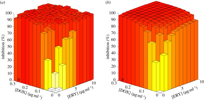
Assuming that the combined effect of both antibiotics can be described by the multiplicative effect of each drug used separately, we were able to capture population-level inhibition of bacteria growing at different drug concentrations, as illustrated in figure 3. Details of the experiment are described in appendix D.

Figure 3.

Population-level inhibition of E. coli growing in a glucose-limited environment and under the effect of different concentrations of doxycycline and erythromycin. (a) Experimental data, (b) model predictions. (Online version in colour.)

Note that the model (2.5a–d) is constructed under the assumption that the population of bacteria is composed of a single bacterial type, although this assumption may hold for short-term experiments, in general the selective pressures imposed by both antibiotics would promote the evolution of multiple antibiotic-resistant phenotypes. For this reason, in the following section, we will extend this model to account for bacteria that can evolve resistance.

2.4. An evolutionary model

As it is clearly difficult to study drug pharmacodynamics and pharmacokinetics in mammalian hosts in the presence of a pathogen and in real time, although perhaps not impossible with advances in imaging techniques [20], the experimental system we study now will use antibiotic deployment strategies in a continuous culture device. Chemostats provide particularly ideal experimental systems to test different profiles of drug use because they can be mechanically adapted to control the supply of different antibiotics dynamically throughout the course of an experiment.

A dense microbial community inhabits the intestine; so in order for invasive pathogens to colonize a niche in the gut, they have to compete with resident commensal bacteria for any available chemical resources. This competition provides an innate protective mechanism termed colonization resistance and although the molecular basis of the interactions between host immune system, invasive pathogens and microbiota remains largely unknown, it is believed that pathogenic bacteria have evolved different strategies for overcoming colonization resistance. For example, by triggering the host's immune response and as a consequence changing the population structure of the gut ecosystem, pathogens may be able to colonize the host [21].

Furthermore, it is known that broad-spectrum antibiotic treatments can decrease the density of the microbial population in the gut considerably [22,23]. As a result, a side effect of chemotherapy may be to disrupt colonization resistance of the host and so increase the risk of infection by an invasive pathogen.

With this in mind, let C = (C₁, … , C_n) and P = (P₁, … , P_m) denote the density of each phenotype of commensal and pathogenic bacteria respectively, where there are n of the former and m of the latter.

Mutation rates representing the changes in commensal phenotypes that occur during cell division are contained in the matrix written as follows: . Here I is the identity matrix representing error-free, clonal reproduction; ε the mutation rate and M a non-negative n-by-n mutation matrix where the ijth entry in M represents the rate at which bacterial phenotype j mutates into bacterial phenotype i when a mutation occurs; the diagonal entries in M are zero as a result. Similarly, the rate of mutation from pathogenic bacterium type j into type i is given by the ijth entry of the non-negative matrix W. As a result, the mutation matrix for the pathogenic population is given by .

If 1 denotes a column vector of those of the appropriate dimension, 1 = (1, 1, … , 1)^T, then

will all be assumed throughout. Both and are assumed to be non-negative and irreducible matrices with 0 < ε < 1.

We shall assume that each bacterial phenotype consumes the limiting resource, at concentration S(t), from the environment with the same affinity for that resource K. So, if μ_i represents the maximal growth rate for bacterial type i, then μ_i = c · V_maxⁱ and the growth rate of that type, Gⁱ(S), will be given by c · uⁱ(S), where uⁱ is a standard Michaelis–Menten term uⁱ(S) = V_maxⁱ S/(K + S). The chemostat's dilution rate will be denoted by d, S₀ will represent the concentration of the limiting resource held in a supply vessel and c is a scalar denoting the conversion rate between resource and biomass.

The state of the evolutionary microbial system under consideration is given by x(t): = (S(t),C(t),P(t)), and the equation governing the evolution of the state in the absence of antibiotics can be written as

2.8a

2.8b

2.8c

with initial conditions x(0) = (S(0),C(0),P(0)). A dot (·) represents the element-by-element or pointwise product between two vectors, parentheses represent inner products in the sense that if u_c(S) = (u_c¹(S), … , u_cⁿ(S)) and u_p(S) = (u_p¹(S), … , u_pⁿ(S)), then

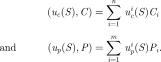Throughout, parentheses will be used in this way to denote inner products.

2.5. Incorporating antibiotics into the chemostat

The basic chemostat device could be readily adapted to have two supply vessels with different antibiotics, as shown in figure 4, whereby each of two supply vessels contains the same concentration of other abiotic resources. This ensures that the deployment of antibiotics does not effect the supply of those resources, including the limiting carbon source.

Figure 4.

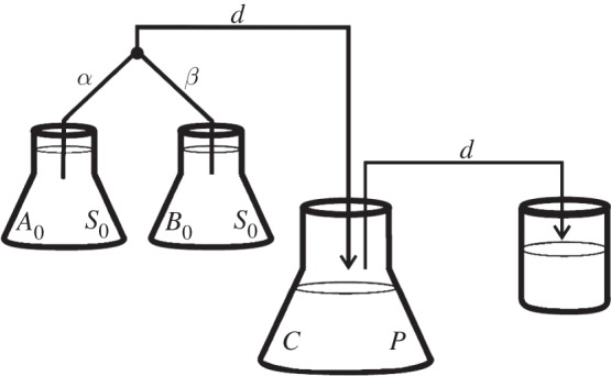
A diagram of a chemostat adapted to supply antibiotic A at a rate α and antibiotic B at a rate β, while maintaining the volume and supply rate of limiting resources (held at concentration S₀) at a constant rate. In this diagram, the constraint α + β = d must apply because fluid and biomass flows from left to right in the diagram along the black lines as indicated by the arrows.

To account for the supply of antibiotics, we extend the state x(t) and write

An evolutionary model for a population of commensal and pathogenic bacteria competing in a single resource-limited environment and subject to the inhibiting effect of two bacteriostatic antibiotics of concentration A and B can now be written as

2.9a

2.9b

2.9c

2.9d

2.9e

with a given initial condition x(0) = (S(0),C(0), P(0), A(0),B(0)). The parameters a and b represent binding rates of each bacterial phenotype to each of the corresponding antibiotic molecules and 1 again denotes a vector of ones, (1, 1, … , 1), of the appropriate dimension.

In the remainder, the system (4a–e) will be written as

for brevity, with the initial condition given by a non-negative vector x(0) = x₀. We want to control the input of both antibiotics into the system throughout an experiment of duration T; so our control variables will be α(t) and β(t), where 0 ≤ t ≤ T, and both control variables are constrained to lie between 0 and d.

2.6. Complete competitive advantage

To mimic a potentially dire situation for the commensal bacteria, we make a number of assumptions. We assume that the wild-type susceptible pathogen (denoted P_s) outcompetes the commensal bacteria (C) in the absence of antibiotics. We then assume a cost of resistance so that, at sufficiently high concentrations of antibiotic, the commensal bacteria are able to outcompete the wild-type pathogen.

However, P_s will be assumed able to evolve resistance, to A say, and the A-resistant pathogenic phenotype (denoted P_a) will then outcompete the commensal. Similarly, if drug B is high in concentration, the B-resistant pathogenic strain (P_b) will also outcompete the commensal. Furthermore, a multi-drug environment imposes strong selective pressures in favour of pathogen mutants resistant to both antibiotics and thus the multi-resistant strain (P_ab) will outcompete C and eventually colonize the host when both A and B are sufficiently high in concentration.

We do not allow the commensal to evolve drug resistance. The rationale for this is that gut commensals form a community composed of many different species and while resistance might evolve in some of these species, we are making a coarse assumption that the commensal microbiota as a whole will behave as if it is mostly composed of susceptible bacteria.

In the situation so-described, there is no value for the concentration vector of the two drugs (A,B) for which the commensals have the highest growth rate, as illustrated in figure 5. In any fixed environment, there exist at least one pathogenic strain that outcompetes the commensal type and we therefore say that pathogens have complete competitive advantage.

Figure 5.

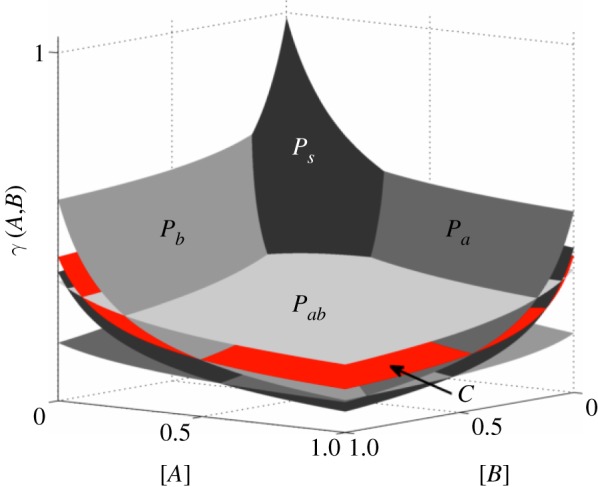
Growth inhibition surfaces for each bacterial phenotype as a function of the concentration of each antibiotic. Note that commensals are not the fittest bacteria in any environment. (Online version in colour.)

In this dire situation, we pose a question that might seem to have an obviously answer in the negative: is there a drug deployment policy that can make the commensals persist as time increases? And if one exists, can we determine an optimal treatment protocol that minimizes the density of pathogens?

2.7. Controlling the chemostat optimally

To minimize the evolution of antibiotic resistance, it is self-evident that the optimal strategy is simply never use antibiotics. This is clearly unreasonable from the perspective of a single host because without treatment the wild-type pathogen will colonize the host. Conversely, drug overdose selects for resistant phenotypes and, as a consequence, decreases the longer-term efficacy of the antibiotic. Then, for a drug deployment policy to be considered long-term optimal, it has to be able to drive the pathogens to extinction while preserving its efficacy.

Taking into consideration the idea that we would like to support the commensal microbiota, we define the healthy state of the system whereby the commensal bacteria are in equilibrium and there are no pathogens present. Ideally, we would steer the system towards the healthy state in such a way that we minimize antibiotic use, but our present question is simpler: do there exist treatment protocols that drive the pathogen density to zero and the commensal to fixation even when the former has complete competitive advantage?

Motivated by techniques from optimal control, we shall use a genetic algorithm to show numerically by example that this is possible by optimizing the treatment protocol with respect to the following objective functional:

2.10

We assume, as shown in figure 4, that the maximum input rate of antibiotic is the same as the dilution rate of the chemostat, so that

We therefore define a set of admissible controls by

and seek an admissible control α* and β* such that the payoff is maximized:

2.11

The existence of the optimal control such that for all is demonstrated in appendix A.

We are interested in the idea of sequential treatments, defined as follows. Two admissible antibiotic deployment protocols, α and β, are said to be sequential if only one of the antibiotics A and B is used at any one time:

2.12

for almost all t between 0 and T. If we define the set of admissible sequential protocols

then Ω_seq is a weak* dense subset of Ω.

To see this, the following construction is useful. Let be a partition of the interval [0,T] so that and let be the space of real-valued, piecewise-constant functions on taking only one of the values either 0 or 1 on each interval of the form (t_k, t_k+1). The set of admissible bang-bang controls

is a subset of, and weak* dense in Ω [24] but Ω_bb ⊂ Ω_seq and so Ω_seq is also weak* dense in Ω.

The outcome of these standard control theoretic ideas is the result that sequential protocols can do as well as any within Ω:

This means that sequential antibiotic deployment protocols that rotate or alternate in turn between two antibiotics can perform as good as any protocol in Ω. In particular, since Ω contains the entire spectrum of combination therapies, from drug A-only to drug-B only, we see that sequential protocols are, in general, at least as good as those that define a fixed proportion of each drug throughout the term of the experiment.

Now the set of sequential protocols is not weak* closed as it contains, for example, the non-sequential 50%-A, 50%-B combination therapy (where α(t) ≡ d/2) in its weak* closure and so the existence of an optimal control within Ω_seq cannot be established in general (one does exist within Ω, though). Notice also that the optimal deployment protocol in Ω is not sequential in general because Ω_seq is a much smaller set than Ω itself.

It follows from the fact that Ω_bb ⊂ Ω is weak* dense that

a property telling us that in order to find near-optimal deployment protocols we need to search only within , possibly for large enough N. This property is exploited in the numerical calculations we perform using a genetic algorithm in §2.8.

2.8. Supporting commensal bacteria with sequential protocols

Seeking a context in which to find highly optimized therapies with two drugs, consider a protocol whereby pathogenic bacteria and commensal bacteria are both introduced into the chemostat at t = 0. In order to colonize the chemostat, the pathogens have to outcompete the commensal bacteria, and to mimic a colonization resistance experiment, we shall assume that the initial population of commensals and wild-type pathogens are at equal densities initially, with no drug-resistant mutants. Recalling our working assumption that pathogens have a greater fitnesses than commensals in an antibiotic-free environment, the pathogens will colonize the host if we fail to use the antibiotics; so, in effect, we are forced into treating with antibiotics in order for the commensal to survive.

Suppose now that pathogens evolve resistance to the antibiotics through two possible point mutations that occur at mutation rate ε where the accumulation of two mutations confers multi-drug resistance. To reflect this, the mutation matrix for the population of pathogenic bacteria is given by the irreducible, stochastic matrix

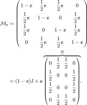As already discussed, the commensal bacteria cannot evolve resistance to antibiotics used and we assume that the pathogen has complete competitive advantage. By controlling the input of antibiotics, we will now attempt to drive the pathogens to extinction while supporting the commensal. The state of the specific model we now use is x = (S, C, P_s, P_a, P_b, P_ab, A,B) and we take advantage of the theoretical results of the previous section by numerically maximizing the objective functional (1) within the space of sequential protocols where w = (0, 1, −1, −1, −1, −1, 0, 0).

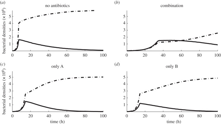
The result of first of the numerical simulations is shown in figure 6, illustrating the dynamics of different drug deployment mechanisms. It is shown that the deployment of just one antibiotic is ineffective and while the best combination strategy is initially effective at suppressing pathogens, it also imposes a severe cost on the commensal population. Indeed, the constant deployment of any two-drug cocktail at any fixed drug ratio will have the consequence that one of the pathogens colonizes the system (figure 6b). It is clear, therefore, that in order to find a drug deployment strategy that can allow the commensals to persist, we have to allow the ratio between drugs to change over time.

Figure 6.

Numerical simulations with the parameter values given in table 1 showing the densities of pathogens (dashed-dotted lines) and commensals (solid lines) throughout an experiment of duration T = 100 h. (a) Bacterial densities (per millilitre) when no antibiotics are used and drug-susceptible pathogens colonize the system. (b) As the two antibiotics are synergistic, a 50–50 combination strategy (equal concentrations of each drug) is most effective at suppressing the density of pathogens. However, commensals are also suppressed, eventually allowing the multi-drug-resistant pathogen to colonize the host. (c,d) Single-drug protocols are ineffective, allowing resistant pathogens to colonize the system.

Although optimal treatments can be obtained for the treatment objective J(α, β) either with an optimization algorithm or by solving the Euler–Lagrange equations associated with this functional, in practice this can be a challenging computational task, particularly when T is large. However, the optimal control for J under the constraint that we must deploy antibiotic at all times is a sequential protocol that can be described as follows. Deploy one antibiotic at the beginning of the experiment until some as yet unknown moment in time when a switch to a different will be needed; a repetition of this process will then define a sequential protocol. While computation of near-optimal controls could be achieved using a variety of different optimization methods, we chose the genetic algorithm described in appendix B.

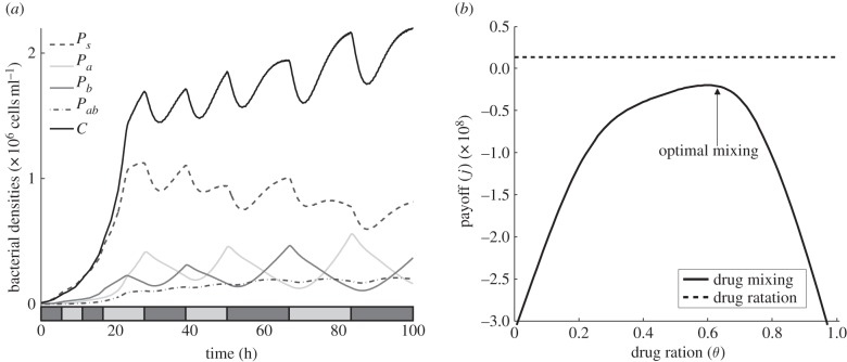
Figure 7 shows the results of applying this algorithm to the model (2.9) where the parameter values are given in appendix E. The result is a sequential protocol whereby the commensals have the highest density at the end of the experiment and this was obtained by numerically maximizing the treatment objective J. The sequential protocol so-obtained is just one from an infinite family of suboptimal controls that outperform all the fixed-ratio combination protocols with respect to the treatment measure J, as shown in figure 7b.

Figure 7.

(a) Bacterial densities under an antibiotic deployment regime determined using a genetic algorithm (see appendix for details). The sequential protocol is represented by the barcode in the bottom of the figure; a light (or dark) box represents the time that drug A (or B) is being deployed at maximal dose during that time interval. Note that commensal bacteria have the highest density of all the types present, despite never being the fittest cell type. (b) The solid line (drug mixing) represents the treatment objective (J) of every possible combination with a fixed ratio between drugs (drug ratio, called θ in the text). The dashed line (drug rotation) shows the payoff of the sequential protocol illustrated in (a). Although it is not the J-optimal treatment, it outperforms even the optimal combination strategy.

3. Discussion

We provided an evolutionary model of a microbial microcosm and used it to evaluate the efficacy of different drug deployment strategies. Our model is derived from kinetic interactions between drugs and their targets, and is consistent with the outcome of an experiment designed to measure the inhibitory effect different concentrations of two antibiotics have on a bacterial population cultured under resource limitation.

We use the model to demonstrate, from well-known optimal control theory, that although commensals may be outcompeted by a rapidly evolving pathogen in any fixed multi-drug environment, we may still be able to design treatment protocols based on the sequential deployment of drugs that exclude the pathogen from the system.

It is noteworthy that in spite of the strong synergistic interaction between the two drugs we considered, the optimal protocol was not to use them in combination. Indeed, even suboptimal but dynamically changing protocols can succeed where fixed-ratio combination therapies fail. Note, however, that although we have focused our study on a drug pair with a synergistic interaction, the analysis supporting the optimality of sequential treatments is independent of the drug interaction profile and therefore also holds when the interaction is antagonistic. We naturally chose to use synergism as a case study because it is the combination preferred in clinical settings.

In order to determine an optimal control, or even a near-optimal controls, we essentially need to have access to complete information about the future dynamics of the system that are not likely to be available in practice. Determining the unfolding dynamics of drug resistance evolution is a difficult task, necessitating vast amounts of genomic data to be processed. An alternative to searching for the optimal protocol could, therefore, be to implement sequential treatment protocols based on partial information of the present state of the system as part of a feedback control.

Depending on the precise goal, we could implement such a feedback as part of a heuristic that allows us to decide upon the best drug usage strategy at each moment in time, based on the information we currently have access to. For instance, a very simple heuristic could be designed based on deploying just one antibiotic into the chemostat, but switching immediately to a different drug if the observed levels of resistance to the current antibiotic are too high. If we denote with τ the sampling time, then we can decide which drug to deploy at time t based on the following rule:

• (i) deploy just one antibiotic into the chemostat (for example, drug A) during the time-interval [t - τ, t);

• (ii) at time t measure the levels of resistance to the current antibiotic used, in this example P_a(t);

• (iii) switch to drug B if P_a(t) > max(P_s(t),P_b(t), P_ab(t)) and deploy this drug for another τ units of time. Otherwise, continue the deployment of drug A and repeat the process.

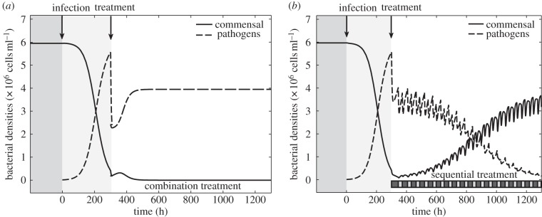
There are many different rules we could write, and we make no claim about the optimality of such rules, but surprisingly this simple feedback heuristic can be sufficient to allow the commensals to persist and drive the pathogens to extinction (figure 8b). This illustrates that even suboptimal sequential protocols can be effective at treating the presence of the pathogen in situations where even the best combination treatment will not work, as shown in figure 8a.

Figure 8.

Numerical simulations of a long-term experiment (T = 1300) of a complete competitive advantage scenario where the numerical values of the parameters used are given in table 1. In both examples, commensals are at equilibrium before susceptible pathogens are introduced into the system (at t = 0). The period when commensals (solid lines) are in equilibrium and there are no pathogens (dashed lines) present has a dark-grey background and the interval of time between initiation of infection and antibiotic deployment (at t = 300) has a light-grey background. The dashed line represents the sum over all pathogenic phenotypes while the solid line represents the density of commensals through the duration of the experiment. (a) All combination treatments select for drug-resistant pathogens, the initial benefit of treatment soon vanishes and pathogens colonize the system, driving the commensal to extinction. (b) In this example, commensals are able to persist with a sequential protocol designed using a feedback control heuristic. (The sequential protocol is illustrated with dark boxes denoting drug B and light boxes denoting drug A at the bottom of the figure.)

The practical implementation of this feedback rule is contingent upon knowing the strain responsible for a bacterial infection and then knowing the relative densities of strains carrying resistance alleles or plasmids. This is biologically detailed information, although the increasing availability of tools to determine such information [25] might make the implementation feedback rules a practical possibility in time.

In summary, these results suggest that in order to remove a fit, adapting pathogen in competition with commensal bacteria, increasing the killing efficacy of the antibiotics is not as important as designing rational deployment strategies that select against drug-resistant pathogens.

Appendix A. Existence of an optimal control

The dependence of equation (2.9a–e) on the control variables is affine in the sense that there is a smooth mapping such that and the objective functional in (2.10) is linear in the state, x, as it can be written in terms of a weight vector, w:

A1

As a result, J : L^∞ × L∞ → is continuous with respect to weak*, L^∞-convergence. Moreover, Ω is a closed, convex subset of L^∞ × L^∞ and so is compact with respect to the weak* topology on L^∞ × L^∞.

Solutions of (2.9a–e) satisfy a control-independent, dissipative bound of the following form: for each initial condition x₀ there is a t′ depending on x₀ such that

A2a

and

A2b

for all t > t′. To see this, define Σ : = S₀ − S − (1/c)× ((1,C(t))+(1,P(t))) and note that the differential inequality (d/dt)Σ ≤ −dΣ follows from (2.9a–e), the bound in (A 2a) now follows. The bounds in (A 2b) are obtained from the inequalities (d/dt)A ≤ d(A₀ − A) and (d/dt) B ≤ d(B₀ − B) satisfied by positive solutions of (2.9a–e).

Theorem A.1. There exists an optimal control such that for all .

Proof. Seeking an optimal control that maximizes the payoff functional defined in (A 1) subject to the system of differential equations given in (2.9a–e), suppose that

for a supremizing sequence of admissible controls , where . This sequence has an associated sequence of state responses that satisfies where for each k.

Because almost everywhere, we can assume without loss of generality that

as k → ∞ because Ω is compact with respect to the weak* topology in .

Owing to the dissipative bound (A 2), there is an M > 0 independent of k such that and so, using , we obtain a k-independent W^1,∞-bound on x_k. We may therefore assume without the loss of generality that in and so, basic compact embedding results allow us to take the latter convergence in . As a result, continuity properties of the nonlinear mapping ℱ can be used to deduce that and . Furthermore,

and so .▪

Appendix B. Genetic algorithm

To compute near-optimal antibiotic deployment protocols, a genetic algorithm searches for near-optimal sequential protocols through the space of bang–bang controls using the following simple strategy. Given a partition of the time-interval [0,T] into n equal sub-intervals, a single drug flows into the chemostat at maximum dose on each sub-interval and a switch of antibiotic may occur at the end of each sub-interval.

The set of all potential switches , can be expressed as a binary string representing ‘yes/no’ switching decisions of length n; this string is called the chromosome, 𝒞, of a given treatment. Each gene, yn_i, can be expressed by allele 0, meaning that the same drug is going to be deployed at the next sub-interval, or by allele 1, meaning that a switch to the other drug is necessary. We therefore associate each chromosome with a bang–bang control strategy α(t; 𝒞) and from this we compute its fitness where and J is computed by solving the differential equation (2.9).

The total number of different sequential protocols to search through is 2ⁿ and the following algorithm was used to determine an optimized control from this set:

• (i) fix a population size N and choose a random initial population of N chromosomes,

  Given define as follows;

• (ii) compute the fitness for each 𝒞_i in the current population;

• (iii) select the fittest chromosomes and reproduce them pair-wise. The chromosome of the resulting offspring is constructed by recombination, inheriting each allele from only one of the parents, where these are chosen randomly for each gene; and

• (iv) mutate a fixed proportion of genes of the population by randomly bit-flipping the alleles of some proportion of chromosome, also randomly chosen.

The population then contains only the fittest N members of the previous generation, their offspring and the mutated chromosomes.

Appendix C. Synergy results from two antibiotics targeting one protein

Motivated by the interaction between rifampicin and closely related drugs such as rifabutin and sorangicin A that reduce transcription rates, consider the following enzymatic model:

C1a

C1b

C1c

C1d

Equation (C 1) describes the concentration of RNA polymerase P, an antibiotic pair A and B that bind to P and the final product mRNA that we denote by M. Messenger RNA is transcribed when P binds to a sigma-factor, here denoted σ and the P_σ complex then binds to the promoter region R of some gene on the bacterial chromosome. With the consumption of ATP, not modelled here, the eventual transcription of M results whereupon the promoter region of the gene, the sigma factor and RNA polymerase unbind from the transcription unit of the gene. The model (C 1) is built on an assumption that both antibiotics, A and B, inhibit the binding of the mature transcription unit, which here is just an RNA polymerase-sigma factor complex, to the promoter region of the gene.

This model does not really describe the details of how these drugs work. To more closely respect the mode of action, we would need to include a cascade of additional terms of the form

Here M₃ and M₅ represent oligomers just a handful of nucleotides long that are the abortive mRNA-like transcripts produced when rifampicin-like drugs are bound to RNA polymerase [26]. However, this more complicated model does not provide any additional theoretical insight into the interaction of drugs targeting the same enzyme; (C 1) is already sufficient to have non-trivial, synergistic drug interactions as we now aim to show.

Assuming mass-action kinetics, from (C 1) we obtain the following model for the time-course of concentrations of each of the agents involved in the transcription of mRNA:

C2a

C2b

C2c

C2d

C2e

C2f

C2g

C2h

C2i

C2j

C2k

where A and B are assumed to be held at constant values during transcription.

Equation (C 2) has constants of integration, namely the total available RNA polymerase

and the totality of gene promoters . Let us now assume that all process have equilibrated so that M is produced at a constant rate in (C 2k), then

C2k

Now, and so with (C 2e) and (C 2f) in equilibrium, we obtain

and

that can be rewritten using the preceding algebraic relationships for and as a function of and :

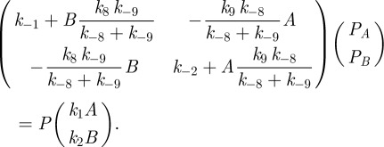C3

The linear equation defined by (C 3) can be solved to give

where κ_A and κ_B are rational functions of the form

where the set of five parameters are various combinations of the rate parameters in (C 1); there is one set of these parameters for each of the two antibiotics.

Continuing with the equilibrium assumptions, follows from (C 2g) but then adding the latter to (C 2h) yields , whence

By defining we can write

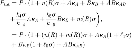and so

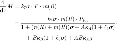a function that we denote by v(A,B).

We finally define γ(A,B) to be the dimensionless reduction in the production rate of mRNA due to A and B, γ (A,B) = v(A,B)/v(0,0), which equals

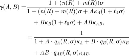C4

We have written in place of for brevity; the functions and are similarly defined as and respectively.

Suppose all the parameters are fixed in (C 4) apart from A and B, so that

where and are constant and strictly positive. To see the function γ(A,B) so-defined defines a synergistic interaction, suppose θ lies strictly between 0 and 1. To ensure a fair comparison in terms of dosage between single-drug and combination environments, we normalize A and B so that , which requires .

We find

and, as a result, whenever and the drugs A and B are therefore said to synergize because they are most effective at reducing the rate of mRNA synthesis when used in combination. The numerical simulations in the paper use the further-restricted inhibition function

which, by the same reasoning, also represents a synergistic interaction.

Appendix D. Experimental methods

The experimental protocol used to obtain the dataset in figures 2 and figure 3 is taken from Hegreness et al. [6] and reproduced here for completeness.

Bacterial Strain

Escherichia coli Strain MC4100 (ordered from the Coli Genetic Stock Center: http://cgsc2.biology.yale.edu/Strain.php?ID=9973) was used. Stocks were made from a single colony picked for an overnight LB-culture and frozen for further use.

M9 Growth Medium

The experiment was then performed in M9 growth medium prepared as follows: part A: 350 , 100 g l⁻¹ ; part B: 29.4 g l⁻¹ trisodium citrate, 50 g l⁻¹ , . Parts A and B were 50 times stock solutions in water, that were sterilzed by autoclaving. For M9 minimal medium, they were diluted in water accordingly. 0.2 per cent glucose and 0.1 per cent casamino acid were added as nutrients for the M9 growth medium.

Antibiotics used

Antibiotics used were erythromycin (from Aldrich, product no. 856193) and doxycycline (Sigma, product no. D9891), two antibiotics known to synergize [6]. Liquid stocks were prepared from powder stocks at 50 mg ml⁻¹. For this purpose, erythromycin hydrate was dissolved in ethanol and doxycycline hyclate in sterile water (afterwards filter sterilized).

Maximal antibiotic concentrations were determined for each antibiotic in preliminary trials as concentrations leading to full inhibition of bacterial growth for 24 h using just one of the antibiotics at a time. The maximum concentration of each drug was 10 µg ml⁻¹ for erythromycin and 0.3 µg ml⁻¹ for doxycycline. For each, 11 dilutions in M9 growth medium ranging from no antibiotic to maximal concentration.

Setup

A grid of all combinations of these concentrations was replicated six times and spread in a systematically randomized way over three 384-well plates at 50 µl per well. Extra wells were filled with growth medium but not inoculated with bacteria for background OD measurements. For inoculation, the wells of a 96-well plate were filled with 100 µl of MC4100 overnight culture, and then a very small subsample was taken by dipping a full 96-rack of 10 µl tips first into the 96-well plate and then into one of the four 96-well subsets of the 384-well plate.

The three plates were sealed with a transparent plastic foil, the liquid was centrifuged down with a short spin and the OD was measured in a Tecan Genios plate reader. They were then grown in a 37°C incubator and shaken at 130 r.p.m. for 24 h. For OD measurements, they were taken out of the incubator every 30 min.

Appendix E. Model parameters

Table 1.

Model parameters.

parameter	description	value
d	chemostat dilution rate	0.6 h−1
ε	rate of point mutations	0.01
c	resource conversion rate	108 cell µg−1
K	bacterial half-saturation constant	0.06 µg ml−1
μi	maximal growth rate of bacterial type i per hour (note c ·Vimax = μi)	μc = 1.16, μs = 1.3, μa = 1, μb = 1, μab = 0.87
S0	resource supply concentration
A0	antibiotic A supply concentration
B0	antibiotic B supply concentration
a	antibiotic A binding rate
b	antibiotic B binding rate
κ1i	maximal growth inhibition of bacterial type i by antibiotic A (dimensionless)
	maximal growth inhibition of bacterial type i by antibiotic B (dimensionless)
κ2i	affinity for antibiotic A of bacterial type i	(all µg ml−1)
	affinity for antibiotic B of bacterial type i	(all µg ml−1)

References

- 1.Nathan C. 2004. Antibiotics at the crossroads. Nature 431, 899–902 10.1038/431899a (doi:10.1038/431899a) [DOI] [PubMed] [Google Scholar]
- 2.Levy A., Marshall B. 2004. Antibacterial resistance worldwide: causes, challenges and responses. Nat. Med. 10, S122–S129 10.1038/nm1145 (doi:10.1038/nm1145) [DOI] [PubMed] [Google Scholar]
- 3.Michea-Hamzehpour M., Pechere J., Marchou B., Auckenthaler R. 1986. Combination therapy: a way to limit emergence of resistance? Am. J. Med. 80, 138–142 10.1016/0002-9343(86)90491-2 (doi:10.1016/0002-9343(86)90491-2) [DOI] [PubMed] [Google Scholar]
- 4.Milatovic D., Braveny I. 1987. Development of resistance during antibiotic therapy. Eur. J. Clin. Microbiol. 6, 234–244 10.1007/BF02017607 (doi:10.1007/BF02017607) [DOI] [PubMed] [Google Scholar]
- 5.Montero A., Ariza J., Corbella X., Domenech A., Cabellos C., Ayats J., Tubau F., Borraz C., Gudiol F. 2004. Antibiotic combinations for serious infections caused by carbapenem-resistant Acinetobacter baumannii in a mouse pneumonia model. J. Antimicrob. Chemother. 54, 1085–1091 10.1093/jac/dkh485 (doi:10.1093/jac/dkh485) [DOI] [PubMed] [Google Scholar]
- 6.Hegreness M., Shoresh N., Damian D., Hartl D., Kishony R. 2008. Accelerated evolution of resistance in multidrug environments. Proc. Natl Acad. Sci. USA 105, 13 977–13 981(doi:10.1073/pnas.0805965105) [DOI] [PMC free article] [PubMed] [Google Scholar]
- 7.Chait R., Craney A., Kishony R. 2007. Antibiotic interactions that select against resistance. Nature 446, 668–671 10.1038/nature05685 (doi:10.1038/nature05685) [DOI] [PubMed] [Google Scholar]
- 8.Yeh P. J., Hegreness M. J., Aiden A. P., Kishony R. 2009. Drug interactions and the evolution of antibiotic resistance. Nat. Rev. Microbiol. 7, 460–466 10.1038/nrmicro2133 (doi:10.1038/nrmicro2133) [DOI] [PMC free article] [PubMed] [Google Scholar]
- 9.Cokol M., et al. 2011. Systematic exploration of synergistic drug pairs. Mol. Syst. Biol. 7, 544. 10.1038/msb.2011.71 (doi:10.1038/msb.2011.71) [DOI] [PMC free article] [PubMed] [Google Scholar]
- 10.Stecher B., et al. 2007. Salmonella enterica serovar Typhimurium exploits inflammation to compete with the intestinal microbiota. PLoS Biol. 5, 2177–2189 10.1371/journal.pbio.0050244 (doi:10.1371/journal.pbio.0050244) [DOI] [PMC free article] [PubMed] [Google Scholar]
- 11.Dethlefsen L., Relman D. A. 2010. Microbes and health sackler colloquium: incomplete recovery and individualized responses of the human distal gut microbiota to repeated antibiotic perturbation. Proc. Natl Acad. Sci. USA 108, 4516–4522 10.1073/pnas.1000087107 (doi:10.1073/pnas.1000087107) [DOI] [PMC free article] [PubMed] [Google Scholar]
- 12.Peña-Miller R., Lähnemann D., Schulenburg H., Ackermann M., Beardmore R. 2011. Selecting against antibiotic-resistant pathogens: optimal treatments in the presence of commensal bacteria. Bull. Math. Biol. 74, 908–934 [DOI] [PubMed] [Google Scholar]
- 13.Andersson D. I., Levin B. R. 1999. The biological cost of antibiotic resistance. Curr. Opin. Microbiol. 2, 489–493 10.1016/S1369-5274(99)00005-3 (doi:10.1016/S1369-5274(99)00005-3) [DOI] [PubMed] [Google Scholar]
- 14.Gagneux S., Long C. D., Small P. M., Van T., Schoolnik G. K., Bohannan B. J. M. 2006. The competitive cost of antibiotic resistance in Mycobacterium tuberculosis. Science 312, 1944–1946 10.1126/science.1124410 (doi:10.1126/science.1124410) [DOI] [PubMed] [Google Scholar]
- 15.Berenbaum M. 1989. What is synergy? Pharmacol. Rev. 41, 93–141 [PubMed] [Google Scholar]
- 16.Greco W., Bravo G., Parsons J. 1995. The search for synergy: a critical review from a response surface perspective. Pharmacol. Rev. 47, 331–385 [PubMed] [Google Scholar]
- 17.Loewe S. 1953. The problem of synergism and antagonism of combined drugs. Arzneimittelforschung 3, 285–290 [PubMed] [Google Scholar]
- 18.Smith H. L., Waltman P. E. 1995. The theory of the chemostat: dynamics of microbial competition. Cambridge Studies in Mathematical Biology Cambridge, UK: Cambridge University Press [Google Scholar]
- 19.Lehar J., et al. 2009. Synergistic drug combinations tend to improve therapeutically relevant selectivity. Nat. Biotech. 27, 659–666 10.1038/nbt.1549 (doi:10.1038/nbt.1549) [DOI] [PMC free article] [PubMed] [Google Scholar]
- 20.Zhao M., Yang M., Baranov E., Wang X., Penman S., Moossa A. R., Hoffman R. M. 2001. Spatial-temporal imaging of bacterial infection and antibiotic response in intact animals. Proc. Natl Acad. Sci. USA 98, 9814–9818 10.1073/pnas.161275798 (doi:10.1073/pnas.161275798) [DOI] [PMC free article] [PubMed] [Google Scholar]
- 21.Stecher B., Hardt W.-D. 2008. The role of microbiota in infectious disease. Trends Microbiol. 16, 107–114 10.1016/j.tim.2007.12.008 (doi:10.1016/j.tim.2007.12.008) [DOI] [PubMed] [Google Scholar]
- 22.Stecher B., Macpherson A. J., Hapfelmeier S., Kremer M., Stallmach T., Hardt W. 2005. Comparison of Salmonella enterica serovar Typhimurium colitis in germfree mice and mice pretreated with streptomycin. Infect Immun. 73, 3228–3241 10.1128/IAI.73.6.3228-3241.2005 (doi:10.1128/IAI.73.6.3228-3241.2005) [DOI] [PMC free article] [PubMed] [Google Scholar]
- 23.Sullivan A., Edlund C., Nord C. 2001. Effect of antimicrobial agents on the ecological balance of human microflora. Lancet Infect. Dis. 1, 101–114 10.1016/S1473-3099(01)00066-4 (doi:10.1016/S1473-3099(01)00066-4) [DOI] [PubMed] [Google Scholar]
- 24.Sussmann H. T. 1972. The bang-bang problem for certain control systems in GL(n,r). SIAM J. Control 10, 470–476 10.1137/0310036 (doi:10.1137/0310036) [DOI] [Google Scholar]
- 25.Bergeron M., Ouellette M. 1998. Preventing antibiotic resistance through rapid genotypic identification of bacteria and of their antibiotic resistance genes in the clinical microbiology laboratory. Clin. Microbiol. 36, 2169–2172 [DOI] [PMC free article] [PubMed] [Google Scholar]
- 26.Xu M., Zhou Y. N., Goldstein B. P., Jin D. J. 2005. Cross-resistance of Escherichia coli RNA polymerases conferring rifampin resistance to different antibiotics. J. Bacteriol. 187, 2783–2792 10.1128/JB.187.8.2783-2792.2005 (doi:10.1128/JB.187.8.2783-2792.2005) [DOI] [PMC free article] [PubMed] [Google Scholar]