Wind selectivity and partial compensation for wind drift among nocturnally migrating passerines

Abstract

A migrating bird’s response to wind can impact its timing, energy expenditure, and path taken. The extent to which nocturnal migrants select departure nights based on wind (wind selectivity) and compensate for wind drift remains unclear. In this paper, we determine the effect of wind selectivity and partial drift compensation on the probability of successfully arriving at a destination area and on overall migration speed. To do so, we developed an individual-based model (IBM) to simulate full drift and partial compensation migration of juvenile Willow Warblers (Phylloscopus trochilus) along the southwesterly (SW) European migration corridor to the Iberian coast. Various degrees of wind selectivity were tested according to how large a drift angle and transport cost (mechanical energy per unit distance) individuals were willing to tolerate on departure after dusk. In order to assess model results, we used radar measurements of nocturnal migration to estimate the wind selectivity and proportional drift among passerines flying in SW directions. Migration speeds in the IBM were highest for partial compensation populations tolerating at least 25% extra transport cost compared to windless conditions, which allowed more frequent departure opportunities. Drift tolerance affected migration speeds only weakly, whereas arrival probabilities were highest with drift tolerances below 20°. The radar measurements were indicative of low drift tolerance, 25% extra transport cost tolerance and partial compensation. We conclude that along migration corridors with generally nonsupportive winds, juvenile passerines should not strictly select supportive winds but partially compensate for drift to increase their chances for timely and accurate arrival.

INTRODUCTION

Wind is known to play a significant role in the timing, intensity, and resultant direction of migratory bird movements (Liechti 2006). Given the ephemeral nature of incident winds, it is reasonable to conceive that migrants would benefit from flexible responses to wind. Such responses should facilitate timely and spatially accurate migration consistently over the years because the consistency of routes and migratory timing apparently impacts population fitness (Newton 2006; Calvert et al. 2009; Shamoun-Baranes et al. 2010).

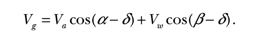
Migration typically involves directed movement, that is, a preferred direction along which the bird wants to travel (Newton 2007). Wind drift can result when crosswinds occur, that is, when winds are not parallel with the preferred direction. The bird can at least partially compensate for wind drift by adjusting its body orientation relative to the ground (hereafter: heading) and possibly its own flight speed relative to the moving air (hereafter: airspeed) (Shamoun-Baranes et al. 2007; Chapman et al. 2011). The resultant speed relative to the ground (ground speed) and direction of travel relative to the preferred direction (drift angle) are determined by computing the vector sum of the wind and the bird’s own velocity (see Methods and Figure 1).

Figure 1.

The classic triangle of velocities (viewed from above) equates the resultant velocity vector relative to the ground to the sum of the air velocity and wind velocity vectors. These vectors are represented by scalar groundspeed Vg, airspeed Va and wind speed Vw, and by angles of drift δ, heading α, and wind incidence β. All angles are measured clockwise from the preferred direction (dashed line). The length of the dotted line perpendicular to the ground speed vector represents the minimum airspeed required to maintain a course with drift angle δ given the wind conditions Vw and β (Equation 2).

Preferred directions can depend on both endogenous properties and various environmental cues. Nocturnal migrants apparently maintain preferred directions through the night using celestial, magnetic, and/or olfactory cues (Holland et al. 2009; Wiltschko and Wiltschko 2009). Because adult passerine migrants have been shown to account for artificial displacements, they can presumably access preferred directions using a navigational map (e.g. Perdeck 1958; Thorup et al. 2007a). Preferred directions of juvenile passerine migrants are often presumed to follow a sequence of endogenous headings in what is termed vector orientation (also known as vector navigation or clock and compass migration; see Berthold and Terrill 1991; Åkesson 2003; Mouritsen 2003). Although there is some evidence that juveniles can compensate for previously experienced drift (Evans 1968; Fitzgerald and Taylor 2008; Thorup et al. 2011), most evidence points to endogenous control being paramount to orientation among juvenile migrants (Perdeck 1958; Thorup et al. 2007a; Wiltschko and Wiltschko 2009).

How nocturnal migrants negotiate spatiotemporal variability in environmental cues and incident winds over numerous flights is less well understood. One possibility is that migrants account for variability in the earth’s magnetic field by re-calibrating their magnetic compass to endogenous or navigational-map-based preferences at dusk and dawn using polarized light cues (Cochran et al. 2004; Muheim et al. 2007, 2009; but see e.g. Chernetsov et al. 2011). To facilitate accurate arrival in variable winds, nocturnal migrants could either select nights and altitudes with winds directly supportive of travel toward destination areas, partially or fully compensate for wind, or both.

That departure and flight decisions are often made on the basis of wind is evident from the number of migrants aloft (e.g. Gauthreaux 1991; van Belle et al. 2007; Schmaljohann et al. 2009). This implies an ability to gauge wind speed, direction or displacement by the wind (Richardson 1990; Liechti 2006; Chapman et al. 2011). However, the minimal wind support migrants should tolerate on departure will depend on wind variability and constraints within the annual routine (Alerstam et al. 2011). Although selecting only supportive winds clearly promotes both accurate travel and fast ground speeds, it also restricts departure opportunities and potentially total migration speed (i.e. including stopovers; hereafter: migration speed). Indeed, the scarcity of favorable winds along major migration routes (Gauthreaux et al. 2005; Kemp et al. 2010) apparently necessitates selection of nonsupportive winds (Alerstam et al. 2011; Alerstam 2011)

Similarly, compensation for incident or previous wind drift may or may not be necessary or advantageous. Full or partial compensation reduces drift instantaneously but may potentially reduce migration speed: because the bird no longer dedicates its entire airspeed to travel along the preferred direction, its transport cost (mechanical flight energy per unit distance) will be higher. If winds are unpredictable, migrants which are able to both navigate and assess the distance remaining to their goal can minimize the transport cost through partial compensation involving adjustment of both heading and airspeed (Alerstam 1979a; Liechti 1995). However, in the special case where crosswinds are precisely balanced over the migratory route, the fastest and most energy-efficient way to arrive at the destination area is to fully drift to maximize the ground speed component along the preferred direction (Alerstam 2011). When spatial variability in winds is predictable, other adaptive behaviors are feasible. Populations could, for example, adopt full drift (FD) behavior with endogenous headings adapted to prevalent large-scale wind patterns. Note that population-mean endogenous headings can therefore differ significantly from the mean travel direction (see e.g. Stoddard et al. 1983 for FD neotropic migration over the Atlantic Ocean). For migrants capable of compensating for previous displacements, it may be adaptive to fully drift at certain altitudes (Alerstam 1979b) or regions (Klaassen et al. 2011) and compensate for the displacement later on.

Although diagnosis of compensation for wind drift presents many pitfalls (Green and Alerstam 2002; Shamoun-Baranes et al. 2007), experimental studies suggest that birds adjust their heading to compensate for wind principally on departure (e.g. Bingman et al. 1982; Liechti 1993). Yet estimates of mean proportional drift throughout the night (sensu Green and Alerstam 2002) among nocturnal radar tracks of passerine migrants are variously suggestive of full or nearly FD (Zehnder et al. 2001; Bäckman and Alerstam 2003) or partial compensation (Karlsson et al. 2010). One radio-tracking study analyzing reaction to wind among individual Catharus thrushes (Cochran and Kjos 1985) concluded that headings were virtually constant through the night and found little evidence of compensation for drift on departure. Due to the difficulty of tracking passerines accurately over entire migratory stages, experimental studies have not been able to reveal the consequences of maintaining constant headings through the night.

This motivates the need to model compensation for wind drift among vector-orienting migrants in a spatially explicit context. Furthermore, the relative effects on migration accuracy of orientation precision, that is, calibration error (Mouritsen 1998; Thorup and Rabøl 2001; Chapman et al. 2011) and of wind drift have not been compared. Spatially explicit, concept-driven migration models (i.e. those based on behavioral rules) can aid us in understanding the cumulative effect of variable winds under various behavioral strategies and vice-versa (Shamoun-Baranes et al. 2010). Spatially explicit models of passerine migration reported in the literature have simulated FD migration among vector-orienting migrants (Stoddard et al. 1983; Erni et al. 2005; Reilly and Reilly 2009) and partial compensation among truly navigating migrants (Vrugt et al. 2007). The aforementioned studies focus on optimal (inheritability of) endogenous heading in nonuniform winds, whereas the latter study focuses primarily on multiobjective optimization among migrants.

In this study, we evaluate the consequences of and relation between wind selectivity and compensation for wind drift among vector-orienting, nocturnally migrating passerines. Wind selectivity is modeled according to how much drift and transport cost a migrant is willing to tolerate on departure. Three airborne behaviors are considered: a FD behavior and two sorts of partial compensation behaviors, one where heading is adjusted to wind and the other where both heading and airspeed are adjusted. We simulated fall migration along the southwesterly (SW) Europeanmigration corridor using a spatially explicit individual-based model (IBM) and 12 years of wind data. Using the IBM, we determined for all three airborne behaviors the effect of maximal tolerances for drift angle (hereafter: drift tolerance) and transport cost (hereafter: transport cost tolerance) on the probability of successfully arriving at the Iberian coast (hereafter: arrival probability) and on migration speed (km d^-1 including stopovers). We test the following hypotheses with the IBM: 1) the probability of successfully arriving at the Iberian coast is highest with low drift tolerance and with partial compensation involving adjustment of both heading and airspeed; 2) migration speeds are highest with behavior which results in fast ground speeds along preferred directions, that is, with low transport cost tolerance and with FD or partial compensation in conjunction with high drift tolerance; 3) populations with mean endogenous headings westward from the migration axis exhibit higher arrival probabilities, reflecting the advantage of adapting to prevalent westerly winds (see e.g. Figure 1 of Liechti 2006), and (4) given the stochastic nature of incident winds, below a given threshold orientation error, the effect of variable winds on arrival probability will outweigh that due to calibration error. To assess the compatibility of the predicted behavior optimizing arrival accuracy (hypotheses 1, 3) and migration speed (hypothesis 2), we estimated the mean wind selectivity, airborne behavior, and endogenous heading among nocturnally migrating passerines along this corridor using radar measurements.

METHODS

Wind selectivity

Here we describe wind selectivity, that is, the wind conditions under which a nocturnal migrant chooses to depart after dusk. It is convenient to describe a migrant’s motion in a framework relative to the preferred direction (Figure 1). Given the airspeed Va, heading α, wind speed VW, and incident wind angle β, the resultant ground speed Vg and drift relative to the preferred direction δ are

(1a)

(1b)

When fully compensating δ = 0°, when fully drifting α = 0° so that , and when partially compensating the resultant drift will lie between 0° and δ0. Depending on wind conditions, the choice of travel direction is often limited: as pointed out by Alerstam (1978), a given course can only be maintained for airspeeds faster than the wind component perpendicular to the direction of travel (the dotted line in Figure 1):

(2)

In our model, wind selectivity is based on the maximum drift angle and transport cost a vector-orienting migrant will tolerate on departure. These tolerances effectively constrain departure and can be viewed as proximate rules, adapted to provide suitable migration schedules given prevalent wind conditions along the migration route. Under given wind conditions, a migrant can adjust its heading α, airspeed Va, or both, to meet these constraints. The drift tolerance Δ is simply the maximum tolerated drift angle:

(3)

For vector-orienting migrants, the transport cost is the mechanical energy expenditure per unit distance travelled along the preferred direction:

where P(Va) represents the required power to fly at that airspeed (Pennycuick 2008). The transport cost tolerance ε is then defined to be the maximum tolerated extra transport cost relative to that in windless conditions

(4)

where represents the most efficient transport cost in windless conditions, that is, when flying at the maximum range airspeed (Pennycuick 2008). Note that the transport cost tolerance ε is dimensionless. With negative values for ε, supportive winds are required for departure. With positive values, selection of some nonsupportive as well as all supportive winds is allowed. For migrants not adjusting airspeed to wind conditions, ε is inversely related to the component of the ground speed along the preferred direction:

(5)

that is, the maximum tolerated extra transport cost is equivalent to a minimum tolerated ground speed component along the preferred direction. In the model, it was assumed that migrants could gauge both drift and transport cost perfectly.

Airborne behaviors

An FD behavior was tested where migrants did not adjust their flight to the wind and thus headed in their preferred direction (α = 0°), flying at maximum range airspeeds. Computationally, this amounted to determining the resultant drift for α = 0° using Equation 1b, and then testing whether the departure constraints were satisfied (Equations 2–4).

We also tested two partial compensation behaviors: migrants exhibiting the first behavior (PC1) flew at maximum range airspeeds and adjusted only their headings, whereas those exhibiting the second behavior (PC2) adjusted both airspeed and heading according to wind conditions. For both behaviors, migrants headed in their preferred direction if the drift was tolerable (Equation 3). Otherwise, migrants partially compensated to minimize drift while still satisfying the transport cost constraint (if this was not possible, they would not depart). This behavior allowed migrants to preferentially minimize transport cost along the preferred direction to potentially enhance migration speed and save energy. The limiting case of zero drift tolerance (Δ = 0°) of course represents full compensation. For partially compensating migrants adjusting both heading and airspeed (PC2 migrants), the combination of airspeed and heading yielding the lowest relative transport cost (Equation 4) was chosen. In the IBM, choices of airspeed and heading were determined using a local golden-section search algorithm (Forsythe et al. 1976).

Individual-based model

We have developed a spatially explicit IBM for passerine migration from the natal area up to a specified arrival region. This model is based on those previously described in Erni et al. (2005) and Vrugt et al. (2007) and is implemented in Matlab. With this model, we can examine reaction to wind in a spatiotemporal context at the individual and population levels and also account for variability in metabolic costs and fuel deposition, that is, mass gain during stopover. Individual migrants were defined by dynamic state variables (Table 1), which were updated in one-hourly steps according to behavioral rules. At each hour, the behavioral rules determined whether a migrant’s current state and local environment (land cover, time of day, incident wind) dictated searching, feeding/resting, or initiation/continuation of flight. Simulation of each migrant continued until the maximum time was reached or until the migrant 1) arrived successfully, 2) died when fuel reserves fell below 0% lean body mass (LBM), or 3) flew outside of the simulated spatial domain.

Table 1.

Principal dynamic state variables used in the IBM

State variable	Units
LBM	kg
Fuel load	kg
Mechanical energy loss (in flight)	J/s
Fuel deposition rate	%/d
Metabolic energy loss	J/s
Activity (1 = flying, 0 = landed, −1 = hindereda)	—
Preferred direction (clockwise from north)	Degrees
Airspeed	m/s
Heading (relative to wind)	Degrees
Ground speed	m/s
Track direction (relative to ground)	Degrees
Drift angle (relative to preferred direction)	Degrees
Current SST	d
Currently refueling	Logical
Arrived	Logical
Current latitude	Degrees
Current longitude	Degrees
distance to coast	km

aHindered individuals are those which could not meet the departure constraints (Equations 2–4) to depart at the previous civil dusk.

Behavioral rules were chosen to incorporate wind selectivity and airborne behavior, as outlined above. The other dynamic processes most relevant to the present study are the calibration of the preferred direction and the departure decision after dusk. These are outlined below. More details of these processes, and those governing flight duration, flight mechanics and stopover behavior, are provided in the Appendix.

Preferred directions were calibrated at the second hour following civil dusk, and departure initiated if the departure constraints were met (Equations 2–4, and see Appendix). Because departure can also depend on fuel load and fuel deposition rate (see e.g. Weber et al. 1998; Schaub et al. 2008), we also implemented a minimum departure fuel load of 15% LBM at each stopover. Calibrated preferred directions relative to geographic North were sampled from a normal distribution centered on the endogenous heading, with a standard calibration error of ~10° (vector length of 0.985; see Batschelet 1981) as a proxy for inherent and environmentally induced variability (Thorup et al. 2007b).

In this study, we simulated first-fall migration of the most numerous trans-Saharan avian migrant, the Willow Warbler (P. trochilus), along the SW European migration corridor(Hedenström and Pettersson 1987; Hahn et al. 2009). Migration was simulated down to the Mediterranean coast, potentially a major ecological barrier (Erni et al. 2003). This facilitated implementation and interpretation of the model in several ways, for example, by avoiding the more complicated behavior needed to cross the Mediterranean Sea (Fransson et al. 2008; Schaub et al. 2008) and the Sahara Desert (e.g. Biebach et al. 1986; Liechti et al. 2003; Schmaljohann et al. 2009).

The modeled spatial domain, arrival area, and temporal domain were chosen to match Willow Warbler migration in Western Europe. The spatial domain included all of Western Europe (22°W–38°E, 35°N–66°N; see Figure 2). The temporal domain was 1 August – 1 November, after which migration was deemed unsuccessful (Hedenström and Pettersson 1987; Asensio and Cantos 1989; Salewski et al. 2002). In the context of vector-oriented migration, and considering fall ring-recovery, orientation and moon-watching data, migrants were considered to have successfully arrived upon reaching the Iberian coast, between 10°W and 3°E and the Atlantic coast of Portugal south of 39°N (Zink 1970; Hilgerloh 1988, 1989; Bruderer and Liechti 1999). This corresponds to assuming a population-mean migration axis between 210° and 220° (Figure 2).Migrants were presumed to identify the Mediterranean coast and stop when within 0.4° (ca. 45 km) using relevant visual and geophysical cues (e.g. Bruderer and Liechti 1998; Fransson et al. 2008; Henshaw et al. 2009). Arrival along the Mediterranean coast further to the east (hereafter: arrival to the east) was considered unsuccessful, given the longer sea and desert crossing, and impossibility of reaching West Africa on endogenous headings.

Figure 2.

Simulation region and endogenous routes for fall migration, with mean fuel deposition rate (rate of mass gain, %/LBM^/h^-1) including metabolic loss, for a Willow Warbler with 30% fuel load (see Appendix). The box represents the natal area, the dark borders along the Iberian coast represent the arrival area and the curved lines represent trajectories without wind influence for endogenous headings of 210°, 215°, and 220°. The radar tracks were measured in an area above northeast Belgium, marked with an O.

Environmental data, consisting of horizontal winds and land cover, were interpolated over the modeled domain. Twelve years of horizontal wind components (1998–2009) at a pressure level of 850 mb were obtained from NOAA NCEP reanalysis data (Kalnay et al. 1996). Wind data were linearly interpolated in space and time from a 2.5° and 6-hourly to 0.5° and hourly resolutions. Land cover classes from the CORINE land cover data set for Europe (Nunes de Lima 2005) were used to estimate fuel deposition rate values at a 0.2° resolution (see Appendix and Figure 2).

Initial conditions, consisting of date of migratory commencement, endogenous heading, initial fuel load (fractional fat mass) and biometric properties, are listed in Table 2. These were based on field data of juvenile Willow Warblers migrating along this corridor (Hedenström and Pettersson 1987; Cramp and Simmons 1992; Schaub et al. 2008). Initial conditions were varied between individuals, but not between years.

Table 2.

Initial conditions, constants, and parameters from IBM simulations

Description	Units	Values
Initial date	d	13 August ± 8a
Initial latitude	Degrees	56.5°N–58°Nb
Initial longitude	Degrees	13.5°E–16.5°Eb
Initial fuel load	—	0.2–0.4b
Lean body mass (LBM)	G	7.6
Wing span	M	0.181
Wing surface area	m2	0.007
Pressure level of flight	mb	850
Minimum departure fuel load	–	0.15
Mean endogenous heading, clockwise from N	Degrees	210°, 215°, 220°, 225°
Drift tolerance	Degrees	0°, 5°, …, 50°
Transport cost tolerance	—	−0.5, −0.25, …, 1.5
SD calibration of endogenous heading	Degrees	0°, 10°, 20°, 30°

Data were derived for juvenile Willow Warbler migration from Cramp and Simmons (1992), Hedenström and Pettersson (1987), Hedenström and Alerstam (1998) and Schaub et al. (2008).

aMean ± SD (normally distributed).

bRange (uniformly distributed).

IBM simulations

We ran simulations for populations exhibiting each airborne behavior and various configurations of wind selectivity, mean endogenous heading, and standard calibration error (see Table 2). Each population consisted of 10 000 individuals. To test the two hypotheses on arrival accuracies, we determined arrival probabilities and migration speeds for all three airborne behaviors and for drift tolerances (Δ, Equation 3)of 0° to 50° in 5° intervals, and transport cost tolerances (ε, Equation 4) of –0.5 to 1.5 in intervals of 0.25. For these simulations, a default mean endogenous heading of 215° and standard calibration error of 10° (vector length of 0.96; Batschelet 1981) were assumed. To test the hypothesis on migration speed, the mean endogenous heading was varied to 210°, 220°, and 225°, and migration simulated for all three airborne behaviors and tolerances. Similarly, to test the fourth hypothesis, simulations with standard calibration errors of 0°, 20°, and 30° (vector lengths of r =1, r = 0.94, and r = 0.86) were run (assuming a mean endogenous heading of 215°). Finally, to ensure that mean arrival probabilities and migration speeds did not significantly differ with simulations greater than 10 000 individuals, we also simulated populations of 30 000 individuals.

Individuals were considered successful if they arrived at the Iberian coast before 1 November. Model results were evaluated according to the fraction of the population arriving on time at the Iberian coast (hereafter: arrival probability) and the median migration speed among successful migrants. To determine the fate of those individuals not arriving at the Iberian coast, we also examined the probabilities of arriving to the east, of perishing over the Atlantic Ocean (hereafter: perishing at sea), and of remaining on land and failing to arrive anywhere along the Mediterranean coast by 1 November (hereafter: failing to arrive by November).

Radar analysis

For comparison with model results, we analyzed radar measurements of nocturnally migrating passerines from a long-term migration monitoring program in Belgium. Radar tracks, consisting of ground speeds and flight directions (hereafter: track directions), were identified using a Thomson CSF long-range medium-power stacked-beam radar (MPR) operated by the Belgian Air Force and located at Glons, Belgium (50°45’N, 5°32’E, see Figure 2). Tracks were identified every half hour using 10 sequential rotations of 10 s each, similarly to the MPR system used operationally for migration research in the Netherlands (Buurma 1995; van Belle et al. 2007; Shamoun-Baranes et al. 2008). Estimated airspeeds and headings were derived by subtracting horizontal wind vectors from the tracks (see Figure 1). Winds were derived using NOAA NCEP reanalysis data at the nearest grid point (50°N, 5°E) and a pressure level of 925 mb (Kalnay et al. 1996); these 6-hourly data were linearly interpolated in time.

To reduce measurement uncertainties in the radar data, several restrictions were imposed before selecting data for analysis. To minimize the influence of ground clutter, analysis was spatially restricted to a northwesterly (NW) subwindow centered at 51°04’N, 4°51’E and covering an area of 850 km² (analogous to van Belle et al. 2007). To reduce uncertainty in flight altitude and hence incident wind, we only considered tracks measured in the lowest beam, which coveredaltitudes between 400 and 1400 m above the ground at the NW subwindow.

To focus on long-distance nocturnal migration of passerines, we restricted analysis according to season, time of day, and estimated airspeed. We therefore analyzed tracks on evenings from 1 August to 30 September in 2006–2009. To match the IBM and to enhance the possibility that tracks pertained to departing migrants, only tracks from the second hour following civil dusk were analyzed. Lastly, only tracks indicative of airspeeds between 8 and 13 m/s were included in the analysis (Bruderer and Boldt 2001; Alerstam et al. 2007). This airspeed restriction also eliminated the possibility that spurious tracks would occur due to rain.

Given the season and location, we expected to find evidence of predominantly but not exclusively SW migration. We therefore examined circular statistics of SW tracks (those with track directions between 215° ± 45°), specifically their circular mean, vector length r and (assuming normally distributed data) equivalent angular deviation (Batschelet 1981). Excluding southeasterly (SE) tracks (i.e. those with track directions between 125° ± 45°) would not bevalid if these migrants represented fully or partially drifting migrants with SW headings. We therefore tested whether meanestimated headings of SW and of SE tracks were significantly different using Fisher’s nonparametric P-test (Fisher 1993; Jones 2010).

Selectivity for wind among SW tracks was examined, as were the estimated distributions of incident drift and relative transport cost. Selectivity was examined according to the distribution of wind speeds and directions relative to the number of tracks during the second hour following civil dusk each night. Drift angles were calculated as the absolute deviation of the track direction from 215°. The relative transport cost of each SW track was estimated using the estimated airspeed and measured groundspeed and drift angle relative to 215°, that is, assuming a preferred direction of 215° and maximum range airspeeds (see Equation 5).

Finally, we estimated the mean endogenous heading and extent of compensation among SW tracks. We used the estimated mean preferred direction as an indicator of mean endogenous heading because early fall passerine migration along this corridor is dominated by juveniles (van der Jeugd et al. 2007; Hahn et al. 2009), which are proposed to vector orient. Mean preferred directions and proportional drift, that is, the ratio of the measured drift angle to that under an FD behavior, were estimated using Method 1 and Equation 3 of Green and Alerstam (2002). As they noted, the estimated proportional drift can be biased by heterogeneity in preferred directions, that is, pseudo-drift. We therefore measured proportional drift for SW and SE tracks separately as well as for all tracks. To the extent that SW and SE tracks represented distinct preferred directions, the separate analysis is valid. In all cases, analysis was done by performing a linear regression of the mean track direction from eight separate wind directional categories (0°–22.5°, 22.5°–45°, etc.) versus the mean track direction minus heading (“wind effect”) for each wind category. Performing regression on mean values rather than individual tracks suppresses spurious correlations between track and wind directions, at the cost of ignoring variability within each category. The y-intercept is an estimate of the mean preferred direction, and the slope btrack an estimate of the proportional extent of drift. A slope of btrack = 0 indicates full compensation and of btrack = 1 FD.

RESULTS

IBM simulations

For all of the simulations (Table 2), arrival probabilities among populations with 10 000 and 30 000 individuals differed by 0.004 or less, and migration speeds by at most 6%. Model results for a specific airborne behavior or endogenous direction are illustrated as a function of wind selectivity, that is, the drift and transport cost tolerances Δ and ε.

The probability of arriving on time at the Iberian coast was highest for drift tolerances below 20°, with maximal probabilities of for all three airborne behaviors (0.51 for FD and 0.53 for PC populations; see Figure 3a). However, whereas arrival probabilities among FD populations decreased rapidly to zero as the drift tolerance approached zero, arrival probabilities among PC1 and PC2 populations were highest for zero drift tolerance, that is, full compensation. Furthermore, PC populations exhibited close to maximal arrival probabilities for a broader range of drift tolerances than FD populations (e.g. >0.45 for Δ~0°–20° vs. 10°–15° with FD). With drift tolerances exceeding 30°, arrival probabilities were similar for all three airborne behaviors (Figure 3a).

Figure 3.

For modeled populations which 1) fully drift, FD, and 2–3) partially compensate (PC1 and PC2), contour plots of (a) probability of arriving at the Iberian coast, (b) probability of failing to arrive by November, that is, remaining on land but not reaching any Mediterranean coast, and (c) migration speed up to the Iberian coast (km d^-1), as a function of wind selectivity, that is, drift tolerance Δ (horizontal axes) and transport cost tolerance ε (vertical axes). See text for details.

The disadvantageous effect of high drift tolerance on arrival probability can also be seen in trajectories of modeled individual migrants. These are shown in Figure 4 for PC1 migrants with transport cost tolerances of ε=1. Individuals with drift tolerances of Δ = 45° clearly exhibit deviations within and between years beyond those observed for this migratory population (Hedenström and Pettersson 1987). Trajectories of individual FD and PC2 migrants varied similarly with drift tolerances, except that FD migrants with zero drift tolerance never arrived.

Figure 4.

Trajectories in (a) 2007 (b) 2008, of a randomly selected group of modeled PC1 migrants maintaining moderate transport cost tolerances (ε = 0.5), and drift tolerances of: 1) Δ = 0°, 2) Δ = 15°, and 3) Δ = 45°. Icons represent the fate of migrants at simulation end: white represents survived, red deceased. Trajectories were plotted in Google Earth using the Google Earth Toolbox for Matlab; latest code available at http://code.google.com/p/googleearthtoolbox/.

Although arrival probabilities were high for populations with low drift tolerances, they were relatively low with negative transport cost tolerance (ε<0) for all three airborne behaviors (Figure 3a). Indeed, most individuals from modeled populations with ε≤–0.25 failed to arrive by November (Figure 3b). For partial compensation populations, very high transport cost tolerance (ε>0.5) resulted in increased mortality over land following initial mass loss during stopover (not illustrated; see Appendix).

Among successfully arriving modeled populations, migration speeds were unlike arrival probabilities enhanced by tolerance of strong drift, but only markedly so among FD populations (Figure 3c). The low migration speeds exhibited by FD populations with low drift tolerance (Δ<10°) were consistent with the high probability of their failing to arrive by November (Figure 3b). Migration speeds were, similarly to arrival probabilities, enhanced by tolerating high transport costs, but less so for ε>0.25. This was true for all three airborne behaviors. Finally, partial compensation was beneficial to migration speed: among simulations with standard calibration error and endogenous heading, PC1 and PC2 populations migrated on average 11% and 17% faster than FD populations. For example, median migration speeds of FD, PC1 and PC2 populations with low drift tolerance (Δ = 10°) and moderate transport cost tolerances ε=0.5 were 68, 117, and 128 km/d, respectively (Figure 3c).

For all three airborne behaviors, populations with mean endogenous headings of 215° exhibited the highest probabilities of successful arrival. Arrival probabilities among modeled populations with mean endogenous headings of 225° were much lower than the rest (maximally 0.31). This is illustrated in Figure 5a for PC1 populations with mean endogenous headings of 210°, 215°, and 225°. As endogenous headings became more easterly, the probability of arrival to the east of the Iberian coast increased and as endogenous headings become more westerly, the probability of perishing at sea (over the Atlantic Ocean) sharply increased (Figure 5b–c).

Figure 5.

For PC1 modeled populations, contour plots of the probability of (a) arriving at the Iberian coast, (b) arriving east of the Iberian coast, and (c) perishing at sea, as a function of wind selectivity, that is, drift tolerance Δ (horizontal axes) and transport cost tolerance ε (vertical axes). In columns (i)–(iii) population mean endogenous heading is varied, and standard calibration error fixed at 10°. In columns (iv)–(v), population mean endogenous heading is 215° while standard calibration error is varied. See text for details.

In terms of orientation accuracy, populations arrived consistently on the Iberian Peninsula only when their standard calibration errors were less than 30°. For example, maximal arrival probabilities among PC1 populations with 30° standard calibration errors were only 0.25 (Figure 5, column v), and the probability of arriving to the east always exceeded that of arriving at the Iberian coast (not shown). Populations with perfect orientation (0° calibration error) exhibited similar arrival probabilities to those with 10° calibration errors but slightly higher when tolerating low drift (maximum 0.58 vs. 0.53; Figure 5, column ii). This ‘‘improvement’’ was smaller than the probability of being drifted away from the Iberian Peninsula (0.30 with perfect orientation; see Figure 5b–c).

Radar analysis

A total of 59 799 tracks on 222 nights were identified to have airspeeds between 8 and 13 m/s during the second hour following civil dusk over the four-year period. More than 85% of the tracks exhibited a southerly component, with track directions exhibiting a circular mean ± angular deviation of 189° ± 56° and a vector-length of r = 0.53 (Figure 6a). The distribution of estimated headings was slightly more westerly but similarly broad (mean 209° ± 49° and r = 0.63; Figure 6b). These distributions were distinctly bi-modal, with discernible SW and SE peaks. Distributions of heading among SW tracks were 230° ± 34° (r = 0.82) as opposed to 156° ± 47° (r = 0.66) among SE tracks (Figure 6c–d). These distributions were significantly distinct (Fisher’s P-test statistic 3.13·10⁸,P < 0.001).

Figure 6.

Circular histograms of radar measurements at Glons, Belgium, of (a) track directions (b) headings (c) headings among SW tracks (track directions between 170° and 260°) (d) headings among SE tracks (80°–170°). The inset to the right represents the relative frequency of wind directions (directions towards which the wind is blowing) during the sampling period. Colors indicate wind direction in 45° intervals (see inset), and the length of each segment is proportional to frequency of occurrence. Directions are clockwise from geographic North.

Winds during the measurement period were predominantly westerly, that is, blowing from the west (0°–180°; see inset Figure 6). A comparison of wind conditions corresponding to the measured tracks and wind conditions during the entire study period indicates that birds avoided flying into the wind: most SW tracks occurred in winds with a strong easterly component (Figures 6a,c), whereas most SE tracks occurred in westerly, although not north westerly, winds (Figure 6d). High wind speeds were also avoided: the average number of SW tracks was 2.9 times higher on nights with wind speeds less than 10.8 m/s^-1 (the four-year mean airspeed) than on nights with stronger winds.

The estimated distributions of drift angle and relative transport cost among SW tracks were indicative of a strong preference for low drift and transport costs, with tolerances ofΔ ~ 20°–30° and ε < 0.5. This can be seen from Figure 7, which depicts the estimated probability distribution and cumulative probability distributions of drift angle and relative transport cost. There was a sharp decline in the number of tracks with drift angles greater than 20° (Figure 7a). Most tracks exhibited negative relative transport costs, and 90% of all tracks had estimated relative transport costs less than 0.25 (Figure 7b).

Figure 7.

Estimated probability densities (left y axes) and cumulative probability densities (right y axes) of (a) absolute drift from 215° (in degrees) and (b) relative transport cost, among SW radar tracks (track directions between 170° and 260°). Probability densities are depicted by solid lines and cumulative probability densities by dashed lines. Relative transport costs were estimated assuming a preferred direction of 215° and (as in Equation 5) maximum-range airspeeds. Positive values of relative transport cost represent nonsupportive winds, and negative values supportive winds.

Based on regression of track direction against “wind effect” (track direction minus heading), both SW and SE tracks were strongly indicative of distinct mean preferred directions and of partial compensation (Table 3). The 95% confidence intervals of the estimated mean preferred direction and proportional drift among SW tracks these were = 216° ± 7°and btrack = 0.51±0.25. For SE tracks, the estimated mean preferred direction was significantly different ( = 136° ± 9°), but not the estimated proportional drift (btrack = 0.42±0.28). Using the entire data set, the estimated proportional drift was suggestive of FD or “overdrift” (heading partly downwind), but both preferred directions and proportional drift exhibited large uncertainties: = 205 ± 55° and btrack = 2.0±2.1.

Table 3.

Regression analysis among radar tracks at Glons, Belgium

	SW tracks	SE tracks	All tracks
Preferred direction (mean ± 95% CI)	216° ± 7°	136° ± 9°	205 ± 55°
Proportional drift btrack(mean ± 95% CI)	0.51±0.25	0.42±0.28	2.0±2.1
Correlation coefficient R	0.80	0.69	0.47
Number of tracks per directional category (range)	277–11.117	19–6238	2246–13.541

Regression of track direction vs. “wind effect” (track direction minus heading) was performed following Green and Alerstam (2002), using eight directional wind categories (0°–22.5°, 22.5°–45°, etc.). SW tracks are for track directions 215° ± 45°, and SE tracks 170° ± 45°. See text for details.

DISCUSSION AND CONCLUSION

The predicted optimal wind selectivity and airborne behavior maximizing arrival probability was largely supported by the IBM. As expected, arrival probabilities were highest with low drift tolerances (Δ < 20°). Therefore, to the extent that higher arrival probability at the Iberian coast is beneficial to population fitness among long-distance migrants along this corridor, for example, through reduced mortality over ecological barriers (Moreau 1972; Strandberg et al. 2009) or enhanced migratory connectivity (Webster and Marra 2005; Stutchbury et al. 2009; Bächler et al. 2010), vector-orienting migrants are predicted to select winds which result in drift angles smaller than 20° on departure. The hypothesized favorability of partial compensation to arrival probability was only partly supported. Arrival probabilities among partial compensation populations were indeed higher than among FD populations for drift tolerance below 30°, but adjustment of both airspeed and heading did not benefit arrival probability compared to adjusting heading alone. The radar analysis was consistent with both partial compensation and a drift tolerance of approximately 20° (Figure 7a). The variability among SW radar track directions (23°) was slightly higher than this estimated tolerance. This is attributable to variability in endogenous heading and calibration error (which we incorporated in the IBM using standard errors of 5° and 10°), and possibly due to reaction to environmental factors such as topography or rain (Cochran and Kjos 1985; Bruderer and Liechti 1998).

The second hypothesis, that migration speed would be maximized by low transport cost tolerance and by fully drifting, was largely refuted. As predicted, modeled migration speeds were highest with high drift tolerances, but not with FD behavior: both PC1 and PC2 populations exhibited higher migration speeds than FD populations, regardless of wind selectivity. Moreover, migration speeds were highest when tolerating moderately high transport cost (ε≥0.5, i.e. tolerating at least 50% higher transport cost than in windless conditions). This was caused by the predominance of unsupportive winds: waiting for supportive winds effected delays which negated the benefit of lower transport costs (higher ground speeds and/or lower energy costs). Therefore, modeled migration speeds were more strongly influenced by the frequency of low-drift departure opportunities than by transport cost per se. This is also evidenced by migration speeds among modeled PC2 populations, which adjusted airspeed to wind conditions to minimize transport cost, being on average only 5% higher than those among PC1 populations. The radar analysis further supports the necessity of selecting some nonsupportive winds ().

Given that arrival probabilities were highest among populations with mean endogenous headings of 215°, we found no support in the IBM for the third hypothesis that adaptation of more westerly endogenous headings facilitates arrival in the prevalently westerly winds. This was related to heightened mortality at sea in the IBM for mean endogenous headings of 225° (Figure 5c) and attributable to the lack of a consistent change in wind direction to redirect migrants consistently landwards (cf. the Atlantic trade winds in neotropical migration, Stoddard et al. 1983). Among real migrants, adoption of contingency plans beyond vector orientation when blown offshore (Mouritsen 2003; Thorup et al. 2011) could possibly facilitate more westerly headings. However, the estimated mean preferred direction among SW tracks = 216° ± 7° implied by the regression analysis is consistent with the IBM results in suggesting that the extent of such adaptation is limited at most. This reinforces the notion that orienting over open water along this corridor is risky (cf. Alerstam and Pettersson 1976; Newton 1998).

The IBM results support the fourth hypothesis that for vector-oriented migration, precision beyond a certain point has a limited effect on migration accuracy (Figure 4a) relative to wind effects. Although model results indicated that standard calibration error should not exceed 20° (r > 0.94), perfectly orienting populations exhibited only slightly higher maximal arrival probabilities than those with standard (10°) orientation errors (0.58 vs. 0.53). Even among perfectly orienting migrants, the bulk of the nonarriving migrants were still drifted away from the Iberian Peninsula (Figure 5a–c). This limited additional benefit of near-perfect orientation could partly account for the observed variability in orientation precision among caged migrants (Thorup et al. 2007b).

It should be stressed that acceptance of nonsupportive winds does not necessarily imply that migrants are not selecting nights for migratory departure on the basis of wind (cf. Schaub et al. 2004; Alerstam et al. 2011) or contradict the fact that the wind selectivity is generally paramount in determining the number of migrants aloft (Erni et al. 2002; van Belle et al. 2007). Indeed, the radar measurements were indicative of a preference for supportive winds (Figures 6c and b), emphasizing how time constraints within the annual routine can necessitate tolerance of nonsupportive winds. Our analysis illustrates that wind selectivity is best considered in the context of the distribution of incident winds (Figure 6) and the resulting transport cost along preferred directions (Figure 7b). It is also important to be aware that preferred directions can deviate significantly from mean headings due to the effect of reaction to prevalent winds (e.g. 216° vs. 230° at Glons). Assuming a preferred direction of 230° at Glons would seriously bias estimates of proportional drift and would result in very different (unsuccessful) migration trajectories according to the IBM (Figure 5a).

Potential sources of uncertainty in analyzing radar measurements also merit consideration. In our analysis, the estimated headings were conceivably affected by the temporal coarseness (6h) in the NCEP wind data, and by the altitudinal uncertainty in the radar data (±500m). However, given the large number of tracks, such inaccuracies would have presumably led to an unbiased but less concentrated distribution of headings, which would not have strongly affected the estimated proportional drift or endogenous heading. The regression analysis illustrates how pseudo-drift can influence analysis of broad front migration tracks, since analyzing all tracks would have implied FD rather than partial compensation. Our analysis is only valid if SW and SE tracks represented distinct groups of migrants or behavioral reactions to wind, which is clearly supported by their almost nonoverlapping distributions.

This study represents the first direct comparison of radar data with IBMs. Given the predominance of juveniles among fall migrants along this corridor, both the IBM and radar data lend support to the proposal of Mouritsen (1998) and Liechti (2006) that juvenile nocturnally migrating passerines partially compensate for drift on departure. The partial compensation behaviors tested here were based on a migrant tolerating drift up to a predetermined angle. Many other behaviors are also plausible (e.g. proportional drift, Liechti 1995; Chapman et al. 2011; Kemp et al 2012). The degree of adaptive partial compensation among species may also vary with morphology or route (cf. Cochran and Kjos 1985), or conceivably within migration corridors (cf. Klaassen et al. 2011). For example, given the higher prevalence of favorable winds along the SW European migration corridor in spring than fall (Kemp et al. 2010), transport cost tolerance along this corridor may be lower in spring. We did not attempt to assess the feasibility of vector-orientated migration per se, and as such did not try to maximize arrival probabilities through, for example, coastal behavior or selection of optimal altitudes (cf. Erni et al. 2003, 2005) or assess population stability (cf. Reilly and Reilly 2009). Finally, the relative influence of wind selectivity, fuel load, and habitat quality on migration speeds among contrasting species, stopover behaviors, and migration routes (cf. Weber et al. 1998; Weber and Hedenström 2000) deserves further investigation.

Long-distance migration involves many inter-related biological processes in a spatially and temporally dynamic environment. In order to make predictions of or interpret observed migration behavior, it is advantageous to integrate locally based behavioral decisions among individuals over larger spatiotemporal and population scales (Guttal and Couzin 2010; Shamoun-Baranes et al. 2010). Predictions from spatial IBMs can be tested in future field experiments, for example by comparing modeled drift angles in incident winds with orientation of radio-tagged passerines. In this study, we have demonstrated that spatially explicit individual-based modeling provides a powerful tool to assess the cumulative effect of reaction to wind conditions en route and the relative merit of different behaviors at the individual and population level.

REFERENCES

- Åkesson S. 2003. Avian long-distance navigation: experiments with migratory birds. In: Berthold P, Gwinner E, Sonnenschein E, editors. Avian migration Berlin (Germany): Springer; p. 471 492 [Google Scholar]
- Alerstam T. 1978. Analysis and a theory of visible bird migration Oikos 30:273 349 [Google Scholar]
- Alerstam T. 1979a. Optimal use of wind by migrating birds: combined drift and overcompensation J Theor Biol 79:341 353 [DOI] [PubMed] [Google Scholar]
- Alerstam T. 1979b. Wind as selective agent in bird migration Ornis Scand 10:76 93 [Google Scholar]
- Alerstam T. 2011. Optimal bird migration revisited J Ornithol 152 (Suppl 1):S5 S23 [Google Scholar]
- Alerstam T, Chapman JW, Båckman J, Smith AD, Karlsson H, Nilsson C, Reynolds DR, Klaassen RHG, Hill JK. 2011. Convergent patterns of long-distance nocturnal migration in noctuid moths and passerine birds Proc R Soc B: Biol Sci 278:3074 3080 [DOI] [PMC free article] [PubMed] [Google Scholar]
- Alerstam T, Rosén M, Båckman J, Ericson E, Hellgren O. 2007. Flight speeds among bird species: allometric and phylogenetic effects PLoS Biol 5:e197 [DOI] [PMC free article] [PubMed] [Google Scholar]
- Alerstam T, Pettersson C-G. 1976. Do birds use waves for orientation when migrating across the sea? Nature 259:205 207 [Google Scholar]
- Asensio B, Cantos FJ. 1989. La migracion postnupcial de Phylloscopus trochilus en el mediterraneo occidental Ardea 36:61 71 [Google Scholar]
- Askew GN, Ellerby DJ. 2007. The mechanical power requirements of avian flight Biol Lett 3:445 448 [DOI] [PMC free article] [PubMed] [Google Scholar]
- Bächler E, Hahn S, Schaub M, Arlettaz R, Jenni L, Fox JW, Afanasyev V, Liechti F. 2010. Year-round tracking of small trans-Saharan migrants using light-level geolocators PLoS ONE 5:e9566 [DOI] [PMC free article] [PubMed] [Google Scholar]
- Bäckman J, Alerstam T. 2003. Orientation scatter of free-flying nocturnal passerine migrants: components and causes Anim Behav 65:987-996 [Google Scholar]
- Batschelet E. 1981. Circular statistics in biology London: Academic Press; [Google Scholar]
- Berthold P, Terrill SB. 1991. Recent advances in studies of bird migration Annu Rev Ecol Sys 22:357 378 [Google Scholar]
- Biebach H, Friedrich W, Heine G. 1986. Interaction of bodymass, fat, foraging and stopover period in trans-Sahara migrating passerine birds Oecologia 69:370 379 [DOI] [PubMed] [Google Scholar]
- Bingman VP, Able KP, Kerlinger P. 1982. Wind drift, compensation, and the use of landmarks by nocturnal bird migrants Anim Behav 30:49 53 [Google Scholar]
- Bruderer B, Boldt A. 2001. Flight characteristics of birds: 1. radar measurements of speeds Ibis 143:178 204 [Google Scholar]
- Bruderer B, Liechti F. 1998. Flight behaviour of nocturnally migrating birds in coastal areas: crossing or coasting J Avian Biol 29:499 507 [Google Scholar]
- Bruderer B, Liechti F. 1999. Bird migration across the Mediterranean. In: Adams N, Slotow R, editors. Proc Intl Ornithol Cong, Durban Johannesburg: BirdLife South Africa; p. 1983 1999 [Google Scholar]
- Buler JJ, Moore FR, Woltmann S. 2007. A multi-scale examination of stopover habitat use by birds Ecology 88:1789 1802 [DOI] [PubMed] [Google Scholar]
- Bulyuk V. 2010. Autumn departure of adult nocturnally migrating passerines from their breeding sites Avian Ecol Behav 17:1 10 [Google Scholar]
- Buurma LS. 1995. Longe-range surveillance radars as indicators of bird numbers aloft Isr J Zool 41:221 236 [Google Scholar]
- Calvert AM, Walde SJ, Taylor PD. 2009. Nonbreeding-season drivers of population dynamics in seasonal migrants: conservation parallels across taxa Avian Conserv Ecol 4:5 [Google Scholar]
- Chapman JW, Klaasen HGK, Drake VA, Fossette S, Hays GC, Metcalfe JD, Reynolds AM, Reynolds DRR, Alerstam T. 2011. Animal orientation strategies for movement in flows Curr Biol 21:R861 870 [DOI] [PubMed] [Google Scholar]
- Chernetsov N. 2006. Habitat selection by nocturnal passerine migrants en route: mechanisms and results J Ornithol 147:185 191 [Google Scholar]
- Chernetsov N, Kishkinev D, Kosarev V, Bolshakov CV. 2011. Not all songbirds calibrate their magnetic compass from twilight cues: a telemetry study J Exp Biol 214:2540 2543 [DOI] [PubMed] [Google Scholar]
- Cochran WW, Kjos CG. 1985. Wind drift and migration of thrushes: a telemetry study Ill Nat Hist Surv Bull 33:297 330 [Google Scholar]
- Cochran WW, Mouritsen H, Wikelski M. 2004. Migrating songbirds recalibrate their magnetic compass daily from twilight cues Science 304:405 408 [DOI] [PubMed] [Google Scholar]
- Cramp S, Simmons KEL. 1992. The birds of the western palearctic Oxford: Oxford University Press; [Google Scholar]
- Ellegren H. 1991. Stopover ecology of autumn migrating bluethroats Luscinia s. svecica in relation to age and sex Ornis Scand 22:340 348 [Google Scholar]
- Erni B, Liechti F, Underhill LG, Bruderer B. 2002. Wind and rain govern the intensity of nocturnal bird migration in central Europe: a log-linear regression analysis Ardea 90:155 166 [Google Scholar]
- Erni B, Liechti F, Bruderer B. 2003. How does a first year passerine migrant find its way? Simulating migration mechanisms and behavioural adaptations Oikos 103:333 340 [Google Scholar]
- Erni B, Liechti F, Bruderer B. 2005. The role of wind in passerine autumn migration between Europe and Africa Behav Ecol 16:732 740 [Google Scholar]
- Evans PR. 1968. Reorientation of passerine night migrants after displacement by the wind Br Birds 61:281 303 [Google Scholar]
- Fisher NI. 1993. Statistical analysis using circular statistics New York: Cambridge University Press; [Google Scholar]
- Fitzgerald T, Taylor P. 2008. Migratory orientation of juvenile yellow-rumped warblers (Dendroica coronata) following stopover: sources of variation and the importance of geographic origins Behav Ecol Sociobiol 62:1499 1508 [Google Scholar]
- Forsythe GE, Malcolm MA, Moler CB. 1976. Computer methods for mathematical computations Englewood (NJ): Prentice-Hall; [Google Scholar]
- Fransson T, Barboutis C, Mellroth R, Akriotis T. 2008. When and where to fuel before crossing the Sahara desert - extended stopover and migratory fuelling in first-year garden warblers Sylvia borin J Avian Biol 39:133 138 [Google Scholar]
- Gauthreaux SA., Jr 1991. The flight behavior of migrating birds in changing wind fields: radar and visual analyses Am Zool 31:187 204 [Google Scholar]
- Gauthreaux SA, Jr, Michi JE, Belser C. 2005. The temporal and spatial structure of the atmosphere and its influence on bird migration strategies. In: Greenberg R, Marra P, editors. Birds of two worlds: the ecology and evolution of migration Baltimore: The John Hopkins University Press; p. 182 194 [Google Scholar]
- Green M, Alerstam T. 2002. The problem of estimating wind drift in migrating birds J Theor Biol 218:485 496 [PubMed] [Google Scholar]
- Gudmundsson GA, Alerstam T. 1998. Optimal map projections for analysing long-distance migration routes J Avian Biol 29:597 605 [Google Scholar]
- Guttal V, Couzin ID. 2010. Social interactions, information use, and the evolution of collective migration Proc Nat Acad Sci 107:16172 16177 [DOI] [PMC free article] [PubMed] [Google Scholar]
- Hahn S, Bauer S, Liechti F. 2009. The natural link between Europe and Africa -2.1 billion birds on migration Oikos 118:624 626 [Google Scholar]
- Hedenström A, Pettersson J. 1987. Migration routes and wintering areas of Willow Warblers Phylloscopus trochilus (L.) ringed in Fennoscandia Ornis Fenn 64:137 143 [Google Scholar]
- Hedenström A, Alerstam T. 1997. Optimum fuel loads in migratory birds: distinguishing between time and energy minimization J Theor Biol 189:227 234 [DOI] [PubMed] [Google Scholar]
- Hedenström A, Rosén M. 2003. Body frontal area in passerine birds J Avian Biol 34:159 162 [Google Scholar]
- Henshaw I, Fransson T, Jakobsson S, Jenni-Eiermann S, Kullberg C. 2009. Information from the geomagnetic field triggers a reduced adrenocortical response in a migratory bird J Exp Biol 212:2902 2907 [DOI] [PubMed] [Google Scholar]
- Hilgerloh G. 1988. Radar observations of passerine trans-Saharan migrants in southern Portugal Ardeola 35:221 232 [Google Scholar]
- Hilgerloh G. 1989. Orientation of trans-Saharan passerine migrants in southwestern Spain Auk 106:501 502 [Google Scholar]
- Holland RA, Thorup K, Gagliardo A, Bisson IA, Knecht E, Mizrahi D, Wikelski M. 2009. Testing the role of sensory systems in the migratory heading of a songbird J Exp Biol 212:4065 4071 [DOI] [PubMed] [Google Scholar]
- Jones TA. 2010. MATLAB functions to analyze directional (azimuthal) data-III: q-Sample inference Comput Geosci 36:520 525 [Google Scholar]
- Kalnay E, Kanamitsu M, Kistler R, Collins W, Deaven D, Gandin L, Iredell M, Saha S, White G, Woollen J, et al. 1996. The NCEP/NCAR 40-year reanalysis project Bull Ameri Meteor Soc 77:437 471 [Google Scholar]
- Karlsson H, Bäckman J, Nilsson C, Alerstam T. 2010. Exaggerated orientation scatter of nocturnal passerine migrants close to breeding grounds: comparisons between seasons and latitudes Behav Ecol Sociobiol 64:2021 2031 [Google Scholar]
- Kemp MU, Shamoun-Baranes J, Van Gasteren H, Bouten W, van Loon EE. 2010. Can wind help explain seasonal differences in avian migration speed? J Avian Biol 41:672 677 [Google Scholar]
- Kemp MU, Shamoun-Baranes J, van Loon EE, McLaren JD, Dokter AM, Bouten W. Quantifying flow-assistance and implications for movement research. J Theor Biol. doi: 10.1016/j.jtbi.2012.05.026. In Press doi: 10.1016/j.jtbi.2012.05.026. [DOI] [PubMed] [Google Scholar]
- Keşapli-Didrickson Ö, Didrickson J, Busse P. 2007. Autumn migration dynamics, body mass, fat load and stopover behaviour of the Willow Warbler (Phylloscopus trochilus) at Manyas Kuscenneti National Park (NW Turkey) Ring 1:67 89 [Google Scholar]
- Klaassen RHGK, Hake M, Strandberg R, Alerstam T. 2011. Geographical and temporal flexibility in the response to crosswinds by migrating raptors. Proc R Soc B: Biol Sci 278(1710):1339 1346 [DOI] [PMC free article] [PubMed] [Google Scholar]
- Ktitorov P, Bairlein F, Dubinin M. 2008. The importance of landscape context for songbirds on migration: body mass gain is related to habitat cover Landsc Ecol 23:16 179 [Google Scholar]
- Liechti F. 1993. Nächtlicher vogelzug im herbst über süddeutschland: winddrift und kompensation J Ornithol 134:373 404 [Google Scholar]
- Liechti F. 1995. Modelling optimal heading and airspeed of migrating birds in relation to energy expenditure and wind influence J Avian Biol 26:330 336 [Google Scholar]
- Liechti F. 2006. Birds: blowin' by the wind? J Ornithol 147:202 211 [Google Scholar]
- Liechti F, Peter D, Komenda-Zehnder S. 2003. Nocturnal bird migration in Mauritania - first records J Ornithol 144:445 450 [Google Scholar]
- Lindström Å, Kvist A. 1995. Maximum energy intake rate is proportional to basal metabolic rate in passerine birds Proc R Soc B: Biol Sci 261:337 343 [Google Scholar]
- Moreau RE. The Palaearctic-African bird migration systems. London: Academic Press; 1972. [Google Scholar]
- Mouritsen H. 1998. Modelling migration: the clock-and-compass model can explain the distribution of ringing recoveries Anim Behav 56:899 907 [DOI] [PubMed] [Google Scholar]
- Mouritsen H. 2003. Spatiotemporal orientation strategies of long-distance migrants. In: Berthold P, Gwinner E, Sonnenschein E, editors. Avian migration Berlin: Springer; p. 493 513 [Google Scholar]
- Muheim R, Åkesson S, Phillips J. 2007. Magnetic compass of migratory Savannah sparrows is calibrated by skylight polarization at sunrise and sunset J Ornithol 148:485 494 [Google Scholar]
- Muheim R, Philips JB, Deutschlander ME. 2009. White-throated sparrows calibrate their magnetic compass by polarized light cues during both autumn and spring migration J Exp Biol 212:3466 3472 [DOI] [PubMed] [Google Scholar]
- Newton I. 1998. Population limitation in birds: London: Academic Press; p. 287 317 [Google Scholar]
- Newton I. 2006. Can conditions experienced during migration limit the population levels of birds? J Ornithol 147:146 166 [Google Scholar]
- Newton I. 2007. The migration ecology of birds London: Academic Press; [Google Scholar]
- Nunes de Lima MV. Land cover updating for the year 2000. Ispra (VA), Italy: Joint Research Centre (DG JRC) & Institute for Environment and Sustainability (IES); 2005. [Google Scholar]
- Pennycuick CJ. 2008. Modelling the flying bird London: Academic Press; [Google Scholar]
- Perdeck AC. 1958. Two types of orientation in migrating Sturnus vulgaris and Fringilla coelebs as revealed by displacement experiments Ardea 46:1 37 [Google Scholar]
- Rayner JMV. 2001. Mathematical modelling of the avian flight power curve Math Method Appl Sci 24:1485 1514 [Google Scholar]
- Reilly RR, Reilly JR. 2009. Bet-hedging and the orientation of juvenile passerines in fall migration J Anim Ecol 78:990 1001 [DOI] [PubMed] [Google Scholar]
- Richardson WJ. 1990. Wind and orientation of migrating birds: a review Cell Mol Life Sci 46:416 425 [DOI] [PubMed] [Google Scholar]
- Salewski V, Bairlein F, Leisler B. 2002. Different wintering strategies of two Palearctic migrants in West Africa a consequence of foraging strategies? Ibis 144:85 93 [Google Scholar]
- Schaub M, Jenni L, Bairlein F. 2008. Fuel stores, fuel accumulation, and the decision to depart from a migration stopover site Behav Ecol 19:657 666 [Google Scholar]
- Schaub M, Liechti F, Jenni L. 2004. Departure of migrating European robins, Erithacus rubecula, from a stopover site in relation to wind and rain Anim Behav 67:229 237 [Google Scholar]
- Schmaljohann H, Liechti F, Bruderer B. 2009. Trans-Sahara migrants select flight altitudes to minimize energy costs rather than water loss Behav Ecol Sociobiol 63:1609 1619 [Google Scholar]
- Shamoun-Baranes J, Bouten W, Buurma L, DeFusco R, Dekker A, Sierdsema H, Sluiter F, Belle JV, Gasteren HV, Loon EV. 2008. Avian information systems: developing web-based bird avoidance models Ecol Soc 13:38 [Google Scholar]
- Shamoun-Baranes J, Bouten W, van Loon EE. 2010. Integrating meteorology into research on migration Integr Comp Biol 50(3):280 292 [DOI] [PMC free article] [PubMed] [Google Scholar]
- Shamoun-Baranes J, van Loon E, Liechti F, Bouten W. 2007. Analyzing the effect of wind on flight: pitfalls and solutions J Exp Biol 210:82 90 [DOI] [PubMed] [Google Scholar]
- Stoddard PK, Marsden JE, Williams TC. 1983. Computer simulation of autumnal bird migration over the western North Atlantic Anim Behav 31:173 180 [Google Scholar]
- Strandberg R, Klaassen RHG, Hake M, Alerstam T. 2009. How hazardous is the Sahara Desert crossing for migratory birds? Indications from satellite tracking of raptors Biol Lett 6:297 300 [DOI] [PMC free article] [PubMed] [Google Scholar]
- Stutchbury BJM, Tarof SA, Done T, Gow E, Kramer PM, Tautin J, Fox JW, Afanasyev V. 2009. Tracking long-distance songbird migration by using geolocators Science 323:896 [DOI] [PubMed] [Google Scholar]
- Thorup K, Rabøl J. 2001. The orientation system and migration pattern of long-distance migrants: conflict between model predictions and observed patterns J Avian Biol 32:111 119 [Google Scholar]
- Thorup K, Bisson I-A, Bowlin MS, Holland RA, Wingfield JC, Ramenofsky M, Wikelski M. 2007a. Evidence for a navigational map stretching across the continental U.S. in a migratory songbird Proc Nat Acad Sci 104:18115 18119 [DOI] [PMC free article] [PubMed] [Google Scholar]
- Thorup K, Rabøl J, Erni B. 2007b. Estimating variation among individuals in migration direction J Avian Biol 38:182 189 [Google Scholar]
- Thorup K, Ortvad T, Rabøl J, Holland R, Tøttrup A, Wikelski M. 2011. Juvenile songbirds compensate for displacement to oceanic islands during autumn migration PLoS ONE 6(3):e17903 [DOI] [PMC free article] [PubMed] [Google Scholar]
- van Belle J, Shamoun-Baranes J, van Loon EE, Bouten W. 2007. An operational model predicting autumn bird migration intensities for flight safety J Appl Ecol 44:864 874 [Google Scholar]
- van der Jeugd H, Schekkerman H, Majoor F. 2007. Het Constant Effort Site project: een vinger aan de pols van populaties van zangvogels Limosa 80:79 84 [Google Scholar]
- Vrugt JA, van Belle J, Bouten W. 2007. Pareto front analysis of flight time and energy use in long-distance bird migration J Avian Biol 38:432 442 [Google Scholar]
- Weber TP, Alerstam T, Hedenström A. 1998. Stopover decisions under wind influence J Avian Biol 29:552 560 [Google Scholar]
- Weber TP, Hedenström A. 2000. Optimal stopover decisions under wind influence: the effects of correlated winds J Theor Biol 205:95 104 [DOI] [PubMed] [Google Scholar]
- Webster MS, Marra PP. 2005. The importance of understanding migratoryconnectivity and seasonal interactions. In: Greenberg R, Marra PP,editors. Birds of two worlds Baltimore: John Hopkins University Press; [Google Scholar]
- Williams TC Williams JMeditors, 1990. The orientation of transoceanic migrants Berlin: Springer; [Google Scholar]
- Wiltschko R, Wiltschko W. 2009. Avian navigation Auk 126(4): 717 743 [Google Scholar]
- Zehnder S, Åkesson S, Liechti F, Bruderer B. 2001. Nocturnal autumn bird migration at Falsterbo, South Sweden J Avian Biol 32:239 [Google Scholar]
- Zink G. 1970. Der Zug europäischer Singvögel. Ein Atlas der Wiederfunde beringter Vögel. Radolfzell: Vogelwarte Radolfzell; [Google Scholar]
Associated Data
This section collects any data citations, data availability statements, or supplementary materials included in this article.