Ozone Uptake During Inspiratory Flow in a Model of the Larynx, Trachea and Primary Bronchial Bifurcation

Abstract

Three-dimensional simulations of the transport and uptake of a reactive gas such as O₃ were compared between an idealized model of the larynx, trachea, and first bifurcation and a second “control” model in which the larynx was replaced by an equivalent, cylindrical, tube segment. The Navier-Stokes equations, Spalart-Allmaras turbulence equation, and convection-diffusion equation were implemented at conditions reflecting inhalation into an adult human lung. Simulation results were used to analyze axial velocity, turbulent viscosity, local fractional uptake, and regional uptake. Axial velocity data revealed a strong laryngeal jet with a reattachment point in the proximal trachea. Turbulent viscosity data indicated that jet turbulence occurred only at high Reynolds numbers and was attenuated by the first bifurcation. Local fractional uptake data affirmed hotspots previously reported at the first carina, and suggested additional hotspots at the glottal constriction and jet reattachment point in the proximal trachea. These laryngeal effects strongly depended on inlet Reynolds number, with maximal effects (approaching 15%) occurring at maximal inlet flow rates. While the increase in the regional uptake caused by the larynx subsided by the end of the model, the effect of the larynx on cumulative uptake persisted further downstream. These results suggest that with prolonged exposure to a reactive gas, entire regions of the larynx and proximal trachea could show signs of tissue injury.

INTRODUCTION

Ozone (O₃), a ubiquitous air pollutant, is responsible for numerous adverse health effects on the respiratory tract including airway hyperresponsiveness^15,27, tissue lesions^13,30, pulmonary edema^8,26, arterial vasoconstriction⁶, myocardial infarction³², and reduced overall lung function^3,20,22. Ozone exposure can also lead to the inhibition of lung development in children^11,19. Epidemiological studies have even suggested an influence of ambient ozone exposure on mortality rates in metropolitan areas^5,11,17.

The exposure-response relationship for inhaled O₃ has been examined by Mudway and Kelly²⁵ who concluded that there is a linear correlation between O₃ exposure and the inflammation of human airway tissue. Hazucha¹⁴ developed quadratic correlations between O₃ exposure and decrements of pulmonary mechanics. Aris et al.⁴ found that ozone exposure at near-ambient and ambient levels induced tissue inflammation in the proximal airways. Postlethwait³¹ et al. further noted that O₃-induced airway damage to the lower airways occurred in a spatially heterogeneous manner that was reproducible from subject to subject. Together, these studies indicate that the health effects of O₃ are directly related to pulmonary exposure, and suggest that the localization of tissue damage derives from the distribution of O₃ uptake.

We hypothesize that the O₃ dose distribution is influenced by flow disturbances created by the laryngeal constriction. Located proximal to the trachea, the larynx is an oddly-shaped organ including multiple constrictions and irregular luminal cross-sections. Several studies have reported the effect of the larynx on pulmonary airflow. Dekker¹⁰ observed that physical models fabricated from laryngeal-tracheal casts experienced laminar-to-turbulent flow transitions at significantly lower flow rates than their straight tube counterparts. Longest and Vinchurkar²³ made similar observations in numerical simulations of particle deposition in the upper airways, while Lin et al.²¹ demonstrated that the turbulence simulated in airway models including a laryngeal segment was absent in models without a laryngeal geometry. Simulations by Martonen et al.²⁴ further revealed that the presence of the larynx affected the flow pattern through several airway generations distal to the upper airways.

To date, few three-dimensional simulations of the uptake of reactive gases such as O₃ have been reported. Kimbell and Subramaniam¹⁸ studied reactive gas uptake patterns in the nasal passages, showing a correlation between simulated uptake rates of formaldehyde and measurements of epithelial cell damage made in vivo. Taylor et al.³⁵ simulated reactive gas uptake in idealized bifurcation geometries, demonstrating the presence of a region of high uptake at the carina of a model bifurcation. The purpose of the current study was to perform computational fluid dynamics (CFD) simulations to evaluate the effect of the human larynx on reactive gas transport and spatial uptake patterns in the large airways during inspiration.

METHODS

Airway Geometry

CFD computations of ozone transport and uptake were performed on a three-dimensional laryngeal model created by joining three distinct regions. The first region, an ellipse-based larynx, was adapted from the work of de Oliveira Rosa and Pereira⁹. This laryngeal region was 4.5 cm in length and included segments representative of the laryngeal entrance, vestibular folds, glottis, and cricoid cartilage. The second region, a cylindrical tube, was assigned a length of 10 cm and a diameter of 2 cm, representative of an adult human trachea. The final region, a 45-degree downstream bifurcation was adopted from the work of Taylor et al.³⁵. Each daughter branch was modeled as a right circular cylinder of length 3.0 cm and diameter 0.7 cm. In total, we shall refer to this composite model as the idealized larynx model (Fig. 1).

Figure 1.

Coronal (upper panel) and sagittal (lower panel) views of idealized larynx model mesh.

For purposes of comparison, CFD simulations were repeated in a second model that incorporated the tracheal and bifurcation regions, but replaced the laryngeal region with a 4.5 cm long proximal extension of the trachea. As such, differences in flow behavior between the two sets of CFD simulations could be attributed to the effects of the laryngeal geometry. We shall refer to this second model as the tubular control (Fig. 2). Table 1 provides a full description for each of these model geometries.

Figure 2.

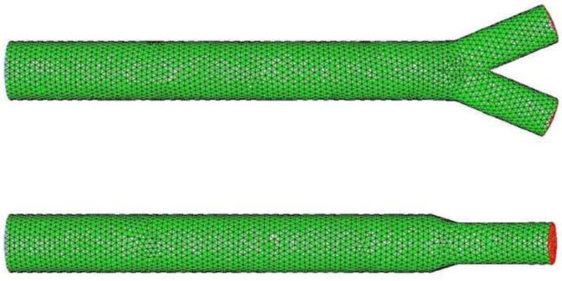
Coronal (upper panel) and sagittal (lower panel) views of tubular control model mesh.

Table 1.

Dimensions of Model Geometries (all units in cm)

	Idealized Larynx		Tubular Control
Axial Position	Coronal Axis	Sagittal Axis	Radius
0.00	1.00	1.00	1.00
1.40	1.00	1.00	1.00
1.52	0.86	1.00	1.00
1.65	0.66	1.00	1.00
1.77	0.64	1.00	1.00
1.90	0.74	1.00	1.00
1.93	0.71	1.00	1.00
1.97	0.50	1.00	1.00
2.00	0.16	1.00	1.00
2.40	0.16	1.00	1.00
2.47	0.36	1.00	1.00
2.61	0.86	1.00	1.00
2.80	1.00	1.00	1.00
4.00	1.00	1.00	1.00
4.25	1.00	1.05	1.00
4.50	1.00	1.00	1.00

Each model was constructed using standard operations in the commercial meshing software GAMBIT, (Ansys Inc., Canonsburg, PA). Tetrahedral mesh elements whose size was equivalent to one-fifth the radius at the flow inlet were used to create a coarse initial grid. Subsequently, a 25-element boundary layer was attached to the walls of the geometry to improve near-wall resolution. The meshes were then exported to Fluent 6.2 (Ansys Inc., Canonsburg, PA) for use in the simulations. Figures 1 and 2 show the final meshes for the idealized larynx model and the tubular control model, respectively.

Governing Equations

Steady incompressible flow of a binary gas mixture of density ρ and viscosity μ is governed by the continuity and Navier-Stokes equations, shown below using index notation.

$$\frac{\partial u_i}{\partial x_i}=0$$ (1)

$$\rho \left(\frac{\partial u_i}{\partial t}+u_j\frac{\partial u_i}{\partial x_j}\right)=-\frac{\partial P}{\partial x_i}+\mu \frac{\partial }{\partial x_j}\frac{\partial u_i}{\partial x_j}$$ (2)

In these equations, u_i and x_i represent the velocity and position vectors, respectively, P denotes the dynamic pressure, and t is time. These equations are supplemented by the following boundary conditions:

1. Model walls: No-slip condition, u_i = 0.

2. Inflow boundary: Uniform axial velocity, u_i = u₀δ_i3, whereu₀ corresponds to physiologically-realistic volumetric flow rates.

3. Outflow boundaries: Zero viscous normal stress

   $$\left(\frac{\partial u_j}{\partial x_i}+\frac{\partial u_i}{\partial x_j}\right)n_i{n}_j=0$$
   (where n is the outward unit normal), and partitioning of volumetric outflows between sibling airway branches in proportion to their cross-sectional areas A₁ and A₂, i.e.

   $$\frac{1}{A_1}\underset{A_1}{\int }{u}_i{n}_{i}dA=\frac{1}{A_2}\underset{A_2}{\int }{u}_i{n}_{i}dA$$

   Since the two sibling airways downstream of the first bifurcation are considered to have the same diameter in this study, the latter condition requires equal flow rates through these two airways.

Because numerous studies have shown that the larynx is capable of generating local turbulence even at sub-turbulent tube Reynolds numbers, the Navier-Stokes and continuity equations were further augmented by the use of the Spalart-Allmaras turbulence model.³³ The Spalart-Allmaras (S-A) model is an empirically derived one-equation turbulence model which relates the Reynolds stress to the mean strain rate through turbulent viscosity²⁹, ν, which is a flow variable whose distribution is given by¹

$$\rho \left(\frac{\partial \nu }{\partial t}+u_i\frac{\partial \nu }{\partial x_i}\right)=\frac{1}{{\sigma }_{\nu }}\left\{\frac{\partial }{\partial x_i}\left[(\mu +\rho \nu )\frac{\partial \nu }{\partial x_i}\right]+C_{b2}\rho {(\frac{\partial \nu }{\partial x_i})}^2\right\}+G_{\nu }-Y_{\nu },$$ (3)

where G_v and Y_v denote the rates of generation and destruction of turbulent viscosity, respectively, and C_b2 and and δ_v are model constants. These quantities are determined as described in the Appendix. The S-A model requires specification of the turbulence intensity¹ I at the flow inlet, a quantity that is expressed as a function of inlet Reynolds number, Re = 2ρu₀r₀/μ, according to

$$I=0.16R{e}^{-\frac{1}{8}}$$ (4)

where r₀ represents the inlet radius.

Finally, for any dilute gas mixture, the concentration distribution of the solute gas is governed by the convection-diffusion equation

$$\frac{\partial C}{\partial t}+u_i\frac{\partial C}{\partial x_i}=D\frac{\partial }{\partial x_i}\frac{\partial C}{\partial x_i}$$ (5)

where D is the binary diffusion coefficient of the solute gas in air, and C is the solute concentration at a given spatial location and time. The following boundary conditions are used in conjunction with the convection-diffusion equation:

1. Model Walls: Zero concentration, C = 0, corresponding to an infinitely fast chemical reaction of a reactive gas (O₃ in this case) with endogenous substrates in the epithelial lining fluid (ELF).

2. Inflow boundary: Uniform inlet concentration profile, C = C₀.

3. Outflow boundaries: Zero diffusive flux, $N=-D{n}_i\frac{\partial C}{\partial x_i}=0$

Numerical Solution

Following importation of the geometric models from GAMBIT into Fluent, the three-dimensional forms of the governing equations were solved using Fluent’s segregated implicit solver. This routine uses the finite volume method with the SIMPLE¹ algorithm for pressure-velocity coupling, and simultaneously solves the Navier-Stokes and continuity equations before solving the convection-diffusion equation. This approach neglects changes in ρ, μ and D due to variations in composition of the gas mixture. Such effects are negligible at the low concentrations of O₃ found in the environment. The solver also implements a second-order accurate flux-limiting upwind scheme to reduce numerical diffusion while avoiding numerical instabilities.

Separate simulations were performed in each model for four physiologically realistic entrance velocities (u₀ = 0.1, 0.3, 1.0, and 3.0 m/s), using the parameter values ρ = 1.225 kg/m³, μ = 1.72×10⁻⁵ kg/m.s, and D = 2.88×10⁻⁵ m²/s. These parameter values correspond to a Schmidt number (Sc = μ/ρD) of 0.49, and the prescribed inlet velocities produce inlet Reynolds numbers of 142, 427, 1,424, and 4,273. A description of the corresponding physiological states is provided in Table 2.

Table 2.

Physiological States Corresponding to Inlet Reynolds Numbers (approximated for an adult human male of normal anatomical dimensions)

Inlet Re	Minute Volume (L)	Physiological State
140	1	Acute Respiratory Distress
430	3	Shallow Breathing/Rest
1400	10	Rest/Light Activity
4300	30	Light/Moderate Exertion

The flow and concentration fields in each simulation were initialized to their values at the inlet. The flow and species conservation equations were then solved iteratively until a maximum convergence error of 10⁻⁶ was achieved by each variable. For the largest inlet Reynolds number considered in this study, the smallest value of the maximum convergence error that could be attained was 10⁻⁵, which is still reasonable.

Resolution

Recommended cell wall distance values for the S-A model fall into two categories: 1 > (wall Y⁺) > 0 and (wall Y⁺) > 30. To assure that the GAMBIT mesh size fell within one of these limits, a series of trial simulations were conducted with different numbers of cells within the wall boundary layer. The results indicated that only the smaller recommended wall distances allowed for fine resolution of boundary flow patterns. In particular, a 25-cell boundary layer mesh at all walls of both model geometries, corresponding to 1 > (wall Y⁺) > 0, was used in all remaining simulations.

Accuracy

The accuracy of the overall numerical method was tested by comparison to existing results for entry flow into a straight tube. In particular, expressions for the dimensionless mass transfer coefficient (the Sherwood number, Sh) in a straight tube of radius r₀ and length L are given by

$${Sh}_{\mathit{laminar}}=0.479{Re}^{\frac{1}{2}}{Sc}^{\frac{1}{3}}{\left(\frac{2r_0}{L}\right)}^{\frac{1}{2}}$$ (6)

for laminar flow, and

$$S{h}_{\mathit{turbulent}}=0.158R{e}^{0.6}S{c}^{-\frac{2}{3}}{\left(\frac{2r_0}{L}\right)}^{0.3}$$ (7)

for turbulent flow, where

$$Sh=\underset{0}{\overset{1}{\int }}\overline{N}d\overline{z}$$ (8)

N̄ is the local wall flux made dimensionless with DC₀/r_0, and z is the dimensionless axial coordinate. The values of Sh obtained from these expressions were compared to the values computed based on the simulations in the tubular control.

The first four rows of Table 3 compare the simulation results for Sh to the predicted values based on Eqs. (6) and (7) for a section of the tube whose outflow boundary was just proximal to the bronchial bifurcation (with L/r₀ = 29). At all but the lowest value of Re, the simulation results lie between the values predicted for the two flow regimes. This is reasonable considering that the S-A turbulent flow model is capable of simulating transitional flows, whereas Eqs. (6) and (7) are only applicable to fully-laminar and fully-turbulent flows, respectively.

Table 3.

Sherwood Numbers for Entry Flow into a Straight Tube

Re	L/r0	Simulated	Predicted (Laminar)	Predicted (Turbulent)
142	29.0	1.13	1.42	1.44
427	29.0	2.70	2.46	2.80
1,424	29.0	5.51	4.50	5.76
4,273	29.0	9.26	7.80	11.13
142	4.5	2.44	2.55	2.05

The simulation result for Re = 142 requires additional explanation. Assuming complete uptake of all inflowing ozone, the calculated Sherwood number would have been 1.19, which is lower than both of the predicted values. This physical impossibility arises because the aspect ratio L/r₀ = 29, for which mass transfer coefficients were predicted, is beyond the range of applicability of Eqs. (6) and (7) at this low Reynolds number. A more reasonable approach is the comparison of predicted and simulated values at L/r₀ = 4.5, shown in the last row of Table 3. For this case, the simulated value is consistent with the predicted value for laminar flow.

Post-Processing

After completion of each CFD simulation, a Fluent user-defined function (UDF) was used to calculate the local dimensionless flux N̄ from the concentration gradients according to Eq. (9). In addition, the individual flux values were scaled by the molar inflow of reactive gas to obtain the local fractional uptake (LFU), as shown in Eq. (10). The expression for LFU is also given in terms of the Peclet number, Pe = Re Sc.

$$\overline{N}=-n_i\frac{\partial \overline{C}}{\partial {\overline{x}}_i}=-\frac{r_0}{C_0}{n}_i\frac{\partial C}{\partial x_i}$$ (9)

$$\mathit{LFU}=\left(\frac{N}{2u_0{C}_0}\right)=\left(\frac{D}{2u_0{r}_0}\right)\overline{N}=\frac{1}{Pe}\overline{N}$$ (10)

A second post-processing algorithm was used to calculate viscosity ratio as a measure of turbulence. Viscosity ratio is defined as the ratio of turbulent viscosity ν (a parameter of the S-A model) to laminar viscosity. Values of viscosity ratio higher than unity indicate a predominantly turbulent flow, while those less than unity correspond to predominantly laminar flow. It should be noted, however, that viscosity ratio does not correlate with turbulence intensity.

Finally, to better visualize the three-dimensional simulations, the results were post-processed to provide surface contour plots as well as plots of cross-sectionally-averaged axial velocity (taken as the component parallel to the direction of the tracheal axis), reactive gas concentration, viscosity ratio, and LFU.

RESULTS

Flow Structure

Figures 3 and 4 are contour maps of dimensionless axial velocity (i.e., local axial velocity normalized by inlet axial velocity) in the coronal cross-section of each model. Inlet Reynolds numbers are shown in an increasing order, with the uppermost color map representing Re = 142 and the lowermost color map representing Re = 4,273. It should be noted that the dimensionless velocities are scaled from 0.0–1.3 in the tubular control and 0.0–7.0 in the idealized larynx.

Figure 3.

Contours of dimensionless axial velocity in the coronal cross-sectional of the tubular control.

Figure 4.

Contours of dimensionless axial velocity in the coronal cross-sectional of the idealized larynx.

In the tubular control (Fig. 3), flow appears stable and symmetric, with a sensitivity to inlet Reynolds number that is apparent in the degree of flow development indicated by the centerline velocity. Namely, the results for Re = 142 show substantial development of flow, whereas progressively higher inlet Reynolds numbers exhibit decreasing degrees of flow development. In the idealized larynx model (Fig. 4), flow appears to be chaotic and relatively insensitive to inlet Reynolds number. In the vicinity of the larynx, flow is dominated by the presence of a laryngeal jet whose velocity approaches seven times the inlet velocity. The bending of this jet causes marked asymmetry in flow and boundary layer disruption throughout the proximal trachea, though differences in flow behavior are significantly attenuated before the first bifurcation.

Figure 5 provides cross-sectional averages for the data seen in the contour maps. As expected, flow in the tubular control is stable and comparable at different axial positions, whereas flow in the idealized larynx model exhibits a sharp peak due to fluid acceleration through the laryngeal jet. Beyond the midpoint of the trachea (10 inlet radii downstream of the inlet), macroscopic flow patterns appear comparable for the two models. Both models also indicate the same small flow disturbance near the first bifurcation.

Figure 5.

Cross-sectional averages of dimensionless axial velocity for the idealized larynx and tubular control models, and the numerical difference between them.

Figure 6 shows the cross-sectional average of the viscosity ratio in each model. In the tubular control, viscosity ratio only exceeds unity in the case of Re = 4,273, where inlet viscosity ratio has a value close to six. At a lower Reynolds number of Re = 1,424, some turbulence is still present near the inlet, whereas for still lower values of Re = 427 and 142, the viscosity ratio is negligible throughout the tubular control.

Figure 6.

Cross-sectional averages of turbulent viscosity ratio for the idealized larynx and tubular control models, and the numerical difference between them.

The behavior of viscosity ratio in the idealized larynx is significantly different. Viscosity ratio values do not decay from an inlet maximum; instead, for the two largest Reynolds numbers, values of viscosity ratio initially decay and then peak in the proximal trachea. The location of peak turbulence corresponds to the site of jet expansion and turbulence generation. This jet turbulence is seen to propagate into the distal trachea in the Re = 1,424 case, and into the first bifurcation in the Re = 4,273 case. In both cases, turbulence subsides by the model exit.

Local Fractional Uptake and Regional Uptake

Coronal surface contours of LFU are shown in Figs. 7 and 8. All LFU contour maps have been scaled to a maximum LFU of 0.02, and portions of the regions colored in red actually exceed this maximum. In both figures, the simulations are shown in a vertical order of increasing Reynolds number. The uppermost contour corresponds to Re = 142 and the lowermost contour corresponds to Re = 4,273. Analysis of Figs. 7 and 8 reveals several trends regarding gas transport.

Figure 7.

Color map of local fractional uptake in the tubular control.

Figure 8.

Color map of local fractional uptake in the idealized larynx.

First, regions of high LFU appear near the inlet of all models. This results from the uniform inlet profiles for both velocity and O₃ concentration. In essence, this imposes a zero boundary layer thickness at the flow entrance, allowing LFU to become infinite. With the development of boundary layers further into the model, LFU begins to decrease. The results of Taylor et al.³⁵ indicate that these inlet regions have little influence upon the remainder of the model.

Second, the mainstem carina is a focal point of high LFU values at all flow rates, whether or not the larynx is present. At the carina, LFU is highest at intermediate flow rates (Re = 427, Re = 1,424). Lower LFU values at the two extremes of the Reynolds number range arise because of different reasons. Low flow rates at Re = 142 allow for depletion of ozone upstream, leaving little ozone to diffuse to the walls of the first bifurcation. The high flow rate at Re = 4,273, on the other hand, leads to a low residence time in which uptake has limited opportunity to occur. It should be noted that, because it is a scaled parameter, LFU behaves differently from the actual surface flux (for which data are not shown). While LFU at the carina peaks at intermediate values of Re, surface flux monotonically increases with Reynolds number, as one would expect.

Third, the inclusion of a larynx somewhat attenuates LFU at the first carina. For fixed Reynolds number, simulations through the idealized larynx geometry showed lower LFU values than simulations through the tubular control geometry. This is most likely due to higher rates of upstream ozone depletion by the larynx, which reduces the concentration driving force for uptake at the carina.

Fourth, simulations through the idealized larynx geometry show sites of high LFU in the larynx and proximal trachea that are not seen in the tubular control. The location of high LFU within the larynx corresponds to an abrupt geometry change at the glottal constriction. On the other hand, the site of high LFU in the proximal trachea occurs within a smooth cylinder, and thus cannot be attributed to a geometric effect. Instead, this hot spot of reactive gas uptake probably corresponds to the reattachment point of the laryngeal jet.

Finally, simulations that include the larynx show a marked asymmetry in LFU until the distal trachea is reached. This results from the asymmetry of internal flow patterns characteristic of the single simulation in Figure 4. Because of the inherent unsteadiness associated with turbulent flow, repeated simulations through the larynx at a fixed Reynolds number resulted in different sites of jet reattachment. Although not completed in this study, we expect that averaging a large number of such simulations would show a ring of elevated LFU on the tracheal wall rather than a single point at which LFU is elevated. This is most likely the case when a person is continuously exposed to ozone for a prolonged period of time. Downstream of the jet reattachment point, where laryngeal flow disturbances subside, the distribution of LFU is symmetric, even in the single simulations shown in Fig. 4.

Figure 9 provides cross-sectional averages of LFU in each model. In the idealized larynx model, peaks are seen at the inlet, vestibular folds, glottis, jet reattachment point, and first carina. In the tubular control, peaks are only seen at the inlet. The difference in LFU between the two models indicates that laryngeal effects predominantly occur in the vicinity of the vestibular folds, glottis, and jet reattachment site. It should also be noted that laryngeal effects depress uptake between the glottis and jet reattachment site—indicating the “insulating” effect of the recirculation regions.

Figure 9.

Cross-sectional averages of local fractional uptake for the idealized larynx and tubular control models, and the numerical difference between them.

Table 4 summarizes the percent cumulative uptake for the idealized larynx, the tubular control, and specific laryngeal effects. Ozone depletion, calculated as the difference in molar flow entering the model inlet versus molar flow passing through a particular downstream cross-section, was normalized by the inlet ozone molar flow to provide cumulative uptake on a percentage basis. The numerical difference between percentage cumulative uptake in the idealized larynx and the tubular control indicates the effect of the larynx. Analysis of Table 4 reveals several trends. First, inclusion of a larynx increases cumulative uptake at all longitudinal distances and at all Reynolds numbers. Second, this increased cumulative uptake monotonically escalates with higher Reynolds numbers. Third, effects of the larynx on cumulative uptake reach maxima within the larynx or trachea in all cases, and begin to subside further downstream within the model.

Table 4.

Cumulative Uptake as a Percent of the Inlet Flow Rate

	Re	Distal Larynx (4.5 cm)	Tracheal Midpoint (9.5 cm)	Distal Trachea (14.5 cm)	Model Exit
Idealized Larynx	142	70.61	88.86	95.89	99.02
	427	47.84	68.80	80.43	89.84
	1,424	30.68	46.71	56.37	67.50
	4,273	21.60	34.60	41.66	50.53
Tubular Control	142	66.37	86.71	94.82	98.74
	427	42.29	62.62	75.78	87.35
	1,424	21.93	35.45	46.35	59.80
	4,273	12.35	19.71	25.97	36.58
Laryngeal Effect on Cumulative Uptake	142	4.23	2.15	1.07	0.29
(% of Inlet Molar Flow)	427	5.54	6.19	4.65	2.49
	1,424	8.74	11.26	10.02	7.70
	4,273	9.25	14.89	15.69	13.95

Table 5 presents regional uptakes normalized by the molar flow entering each region, rather than that entering the model as a whole. This removes the effects of O₃ depletion by upstream airways. Thus, these data represent regional uptake efficiency. The laryngeal effect shown in Table 5 may be attributed to changes in the local flow structure within the model. Several trends are exhibited by the uptake efficiency. First, inclusion of a larynx consistently enhances regional uptake efficiency (enhancements greater than 1%, deemed important, have been highlighted in Table 5). Second, inlet Reynolds number has a strong influence on enhancement in the overall model, as well as within the laryngeal region and proximal trachea. Enhancement is greatest at the highest Reynolds numbers in the overall model, the larynx, and the proximal trachea. Third, the larynx causes little enhancement of regional uptake in the distal trachea, and essentially no enhancement in the bifurcation region at any Reynolds number.

Table 5.

Regional Uptake as a Percentage of the Regional Inlet Molar Flow Rate

	Re	Overall	Larynx	Proximal Trachea	Distal Trachea	Bifurcation
Idealized Larynx	142	99.02	70.61	62.10	63.09	76.22
	427	89.84	47.84	40.19	37.27	48.08
	1,424	67.50	30.68	23.13	18.13	25.51
	4,273	50.53	21.60	16.58	10.80	15.20
Tubular Control	142	98.74	66.37	60.48	61.01	75.63
	427	87.35	42.29	35.22	35.22	47.77
	1,424	59.80	21.93	17.32	16.89	25.07
	4,273	36.58	12.35	8.40	7.80	14.33
Laryngeal Enhancement of Uptake Efficiency	142	0.29	4.23	1.63	2.08	0.59
	427	2.49	5.54	4.97	2.06	0.30
	1,424	7.70	8.74	5.82	1.24	0.44
	4,273	13.95	9.25	8.18	3.00	0.87

^*Proximal trachea refers to the first 5 cm of trachea and distal trachea refers to the final 5 cm.

DISCUSSION

Model Assumptions

The S-A turbulence model was designed primarily for use in aerospace applications, particularly for unbounded flows. As a nascent system of governing equations, the efficacy of the S-A model has yet to be systematically checked in other possible flow conditions. However, the suitability of the S-A model in simulating respiration has been verified in previous studies by Nithiarasu et al.²⁸. Additionally, the S-A system has shown the capability of accurately recreating jet flow, of simulating adverse pressure gradient effects, of exhibiting laminar-to-turbulent transitions—all necessary components for laryngeal simulation. Although work by Suh and Frankel found the S-A turbulence model incapable of simulating the Coanda effect in two-dimensions³⁴, our work shows that such an assertion does not apply when simulations are conducted for three-dimensional flow. Furthermore, the use of the S-A turbulence model in the current study reduced computational costs relative to the k-ω or other, more conventional, two-equation systems.

The selection of flat inlet velocity and concentration profiles in the present simulations results from consideration of the upstream airway anatomies. Irregularities in the configuration of the more proximal airways suggest that flow entering the larynx will not be fully-developed. Furthermore, the results of Taylor et al.³⁵ indicate that entrance profiles actually have little impact upon behavior within the remainder of the model.

In contrast to the tidal flow that is actually present during normal breathing, these simulations examined O₃ uptake during inspiration alone. This approach was necessitated by the lack of realistic boundary conditions at the distal end of the model during expiration. Because of its extreme reactivity, however, the majority of O₃ is absorbed into respiratory tissue during inspiration, so little information regarding O₃ dose distribution is lost by disregarding expiration. To avoid the difficulty and uncertainties associated with the simulation of unsteady turbulence generation, the present work was also restricted to steady flow conditions. Nevertheless, the steady-state snapshots of O₃ distribution that have been obtained at various inspiratory flow rates do provide an adequate approximation of the range of uptakes possible during a more realistic inspiratory flow waveform.

The selection of a zero-concentration boundary condition at the model walls is equivalent to assuming that the rate of chemical reaction at the airway wall is “infinitely fast” compared to the rate of diffusion of ozone to the airway wall. This assumption is only valid for highly reactive gases. Although O₃ is quite reactive with antioxidants and other substrates in the mucous lining layer of the airways, great disparities exist in published estimates of its rate constants. While the use of an infinitely fast wall reaction probably overestimates the heterogeneity of uptake patterns, it nevertheless provides an indication of where hot spots of reactive gas dose may occur.

The use of an idealized laryngeal geometry also merits additional discussion. Work by Brouns et al⁷. suggests that simulations using realistic glottal apertures may reveal features of flow entirely absent in simulations using idealized models. Intrasubject variation in laryngeal anatomy and cyclic changes in larynx geometry during tidal breathing would also influence the characteristics of the downstream air flow. The exact pattern of O₃ uptake in the real respiratory tract would therefore be different from the pattern predicted by simulations in the idealized larynx model. Nevertheless, the presence and approximate location of key features, such as hot spots of O₃ uptake, would likely remain the same in both cases.

Uptake Patterns

The pattern of local fractional uptake at the primary bronchial bifurcation found in this study is in good agreement with those reported by Taylor et al.³⁵ for isolated single airway bifurcations. We observed carinal hotspots at all inlet Reynolds numbers, whether or not the larynx was present. However, when the larynx was present, the magnitude of the hot spot was diminished because of the increased upstream depletion of O₃.

Two new hot spots were observed in the course of the simulations. The first of these occurred at the glottal constriction, where abrupt geometry changes caused a disruption of the velocity field. The consequent thinning of the concentration boundary layer at the airway wall decreased the mass transfer resistance, thereby increasing the local uptake rate. The second new hot spot was found in the proximal trachea at the reattachment region of the laryngeal jet. Because the boundary layer is very thin in this region, we expect a high local uptake rate. A third potential hot spot was observed at the vestibular folds, though non-uniformities in local uptake were decidedly less pronounced there.

Laryngeal effects on reactive gas uptake closely mirror laryngeal effects previously reported for particle deposition. Based on computer simulations, Xi and Longest³⁶ reported that the degree of realism incorporated into a computational model notably affected the accuracy of calculations of flow structure, turbulence, and particle deposition. These investigators found that realistic models aligned more closely with experimental data.

Cumulative uptakes of O₃ tended to decrease with increasing Reynolds number, suggesting a deeper penetration of inhaled ozone into the distal lung at higher inspiratory flows. This is in agreement with the experimental observations of Hu et al.¹⁶ on human subjects.

Conclusion

The results of this study suggest that the larynx may be particularly susceptible to injuries caused by the inhalation of reactive gases such as O₃. Local fractional uptake values are extremely high in the vicinity of the glottal constriction, and are also significantly elevated near the vestibular folds. Additionally, due to the presence of the laryngeal jet, additional sites of injury may appear throughout the proximal trachea.

NOMENCLATURE LIST.

Nomenclature
A	=	wall surface area	m2
C	=	concentration	mol/L
C0	=	inlet concentration	mol/L
D	=	diffusion coefficient	2.88 ×10−5 m2/s
d0	=	inlet diameter	m
I	=	turbulence intensity
L	=	axial position/distance	m
Ni	=	surface flux	mol/m2-s
ṅ	=	molar flow rate	mol/s
$\overline{\stackrel{.}{n}}$	=	dimensionless local wall flux	Equation 9
P	=	hydrodynamic pressure	Pa
Q	=	volumetric flow rate	m3/s
r	=	radius	m
r0	=	inlet radius	m
t	=	time	s
ui	=	velocity vector	m/s
u0	=	inlet velocity	m/s
xi	=	position vector	m
z̄	=	dimensionless axial coordinate	--
Pe	=	Peclet Number	u0d0/D
Re	=	Reynolds Number	u0d0/υ
Sc	=	Schmidt Number	υ/D
Sh	=	Sherwood Number	Equations 6–8
	=
Greek Letters
ρ	=	density	1.225 kg/m3
μ	=	viscosity	1.72 × 10−5 kg/m-s
υ	=	kinematic viscosity	1.4 × 10−5 m2/s
	=	eddy viscosity [S-A]	m2/s
S-A Constants
Gυ	=	eddy viscosity generation term	kg/m-s2
Yυ	=	eddy viscosity destruction term	kg/m-s2
Sv	=	eddy viscosity source term	0 kg/m-s2
δυ	=	model constant	0.667
κ	=	model constant	0.4187
Cb1	=	model constant	0.1355
Cb2	=	model constant	0.622
Cv1	=	model constant	7.1
Cw2	=	model constant	0.3
Cw3	=	model constant	2

APPENDIX 1: THE SPALART-ALLMARAS TURBULENCE MODEL

The Spalart-Allmaras turbulence model may be fully defined by the following series of equations¹,²:

$$\rho \left(\frac{\partial \nu }{\partial t}+u_i\frac{\partial \nu }{\partial x_i}\right)=\frac{1}{{\sigma }_{\nu }}\left\{\frac{\partial }{\partial x_i}\left[(\mu +\rho \nu )\frac{\partial \nu }{\partial x_i}\right]+C_{b2}\rho {(\frac{\partial \nu }{\partial x_i})}^2\right\}+G_{\nu }-Y_{\nu }$$

$${\mu }_t=\rho \nu f_{v1}({\mu }_t=\text{turbulent}\text{viscosity})$$

$$f_{v1}=\frac{{\chi }^3}{{\chi }^3+C_{v1}^3}$$

$$\chi \equiv \nu /(\mu /\rho )$$

Generation

$$G_v=C_{b1}\rho \stackrel{\sim }{S}\upsilon$$

$$\stackrel{\sim }{S}\equiv S+\frac{\nu }{{\kappa }^2{d}^2}{f}_{v2}(d=\text{wall}\text{distance})$$

$$f_{v2}=1-\frac{\chi }{1+\chi f_{v1}}$$

$$S\equiv \sqrt{2{\mathrm{\Omega }}_{ij}{\mathrm{\Omega }}_{ij}}+2.0min(0,\sqrt{2S_{ij}{S}_{ij}}-\sqrt{2{\mathrm{\Omega }}_{ij}{\mathrm{\Omega }}_{ij}})$$

$${\mathrm{\Omega }}_{ij}=\frac{1}{2}(\frac{\partial u_j}{\partial x_i}-\frac{\partial u_i}{\partial x_j})$$

$$S_{ij}=\frac{1}{2}(\frac{\partial u_j}{\partial x_i}+\frac{\partial u_i}{\partial x_j})$$

Destruction

$$Y_v=C_{w1}\rho f_w{(\frac{v}{d})}^2$$

$$C_{w1}=\frac{C_{b1}}{{\kappa }^2}+\frac{1+C_{b2}}{{\sigma }_{\nu }}$$

$$f_w=g{[\frac{1+C_{w3}^6}{g^6+C_{w3}^6}]}^{\frac{1}{6}}$$

$$g=r+C_{w2}(r^6-r)$$

$$r\equiv \frac{\nu }{\stackrel{\sim }{S}{\kappa }^2{d}^2}$$

Model Constants

$${\sigma }_{\nu }=0.667$$

$$\kappa =0.4187$$

$$C_{b1}=0.1355$$

$$C_{b2}=0.622$$

$$C_{v1}=7.1$$

$$C_{w2}=0.3$$

$$C_{w3}=2$$

References

- 1.Fluent 6.3 Users Guide. Lebanon, NH: Fluent Inc; 2006. [Google Scholar]
- 2.FLUENT CFD. Lebanon, NH: Ansys Inc; 2007. [Google Scholar]
- 3.Adams WC, Schelegle ES. Ozone and high ventilation effects on pulmonary function and endurance performance. Journal of Applied Physiology. 1983;55(3):805–812. doi: 10.1152/jappl.1983.55.3.805. [DOI] [PubMed] [Google Scholar]
- 4.Aris RM, Christian D, et al. Ozone-induced airway inflammation in human subjects as determined by airway lavage and biopsy. American Review of Respiratory Disease. 1993;148(5):1363–1372. doi: 10.1164/ajrccm/148.5.1363. [DOI] [PubMed] [Google Scholar]
- 5.Bell ML, McDermott A, et al. Ozone and Short-term Mortality in 95 US Urban Communities, 1987–2000. Journal of the American Medical Association. 2004;292(19):2372–2378. doi: 10.1001/jama.292.19.2372. [DOI] [PMC free article] [PubMed] [Google Scholar]
- 6.Brook RD, Brook JR, et al. Inhalation of Fine Particulate Air Pollution and Ozone Causes Acute Arterial Vasoconstriction in Healthy Adults. Circulation. 2002;105(13):1534–1536. doi: 10.1161/01.cir.0000013838.94747.64. [DOI] [PubMed] [Google Scholar]
- 7.Brouns M, Verbanck S, et al. Influence of glottal aperture on the tracheal flow. Journal of Biomechanics. 2007;40(1):165–172. doi: 10.1016/j.jbiomech.2005.10.033. [DOI] [PubMed] [Google Scholar]
- 8.Cheng P, Boat T, et al. Differential effects of ozone on lung epithelial lining fluid volume and protein content. Experimental Lung Research. 1995;21(3):351–365. doi: 10.3109/01902149509023713. [DOI] [PubMed] [Google Scholar]
- 9.de Oliviera Rosa M, Pereira JC. Towards full-scale three-dimensional larynx simulation. International Conference on Voice Physiology and Biomechanics 2004 [Google Scholar]
- 10.Dekker E. Transition between laminar and turbulent flow in human trachea. Journal of Applied Physiology. 1961;16(6):1060–1064. doi: 10.1152/jappl.1961.16.6.1060. [DOI] [PubMed] [Google Scholar]
- 11.Frischer T, Studnicka M, et al. Lung Function Growth and Ambient Ozone. A Three-Year Population Study in School Children. American Journal of Respiratory and Critical Care Medicine. 1999;160(2):390–396. doi: 10.1164/ajrccm.160.2.9809075. [DOI] [PubMed] [Google Scholar]
- 12.Goldberg MS, Burnett RT, et al. Associations between Daily Cause-specific Mortality and Concentrations of Ground-level Ozone in Montreal, Quebec. American Journal of Epidemiology. 2001;154(9):817–826. doi: 10.1093/aje/154.9.817. [DOI] [PubMed] [Google Scholar]
- 13.Harkema J, Hotchkiss J. Ozone-induced proliferative and metaplastic lesions in nasal transitional and respiratory epithelium: Comparative pathology. Inhalation Toxicology. 1994:6. [Google Scholar]
- 14.Hazucha MJ. Relationship between ozone exposure and pulmonary function changes. Journal of Applied Physiology. 1987;62(4):1671–1680. doi: 10.1152/jappl.1987.62.4.1671. [DOI] [PubMed] [Google Scholar]
- 15.Holtzman MJ, Fabbri LM, et al. Time course of airway hyperresponsiveness induced by ozone in dogs. Journal of Applied Physiology. 1983;55(4):1232–1236. doi: 10.1152/jappl.1983.55.4.1232. [DOI] [PubMed] [Google Scholar]
- 16.Hu SC, Ben-Jebria A, et al. Longitudinal distribution of ozone absorption in the lung: effects of respiratory flow. Journal of Applied Physiology. 1994;77(2):574–583. doi: 10.1152/jappl.1994.77.2.574. [DOI] [PubMed] [Google Scholar]
- 17.Jerrett M, Burnett RT, et al. Long-Term Ozone Exposure and Mortality. New England Journal of Medicine. 2009;360:1085–1095. doi: 10.1056/NEJMoa0803894. [DOI] [PMC free article] [PubMed] [Google Scholar]
- 18.Kimbell JS, Subramaniam RP. Use of Computational Fluid Dynamics Models for Dosimetry of Inhaled Gases in the Nasal Passages. Inhalation Toxicology. 2001;13(5):325 – 334. doi: 10.1080/08958370151126185. [DOI] [PubMed] [Google Scholar]
- 19.Kopp MV, Bohnet W, et al. Effects of ambient ozone on lung function in children over a two-summer period. European Respiratory Journal. 2000;16(5):893–900. doi: 10.1183/09031936.00.16589300. [DOI] [PubMed] [Google Scholar]
- 20.Korrick SA, Neas LM, et al. Effects of ozone and other pollutants on the pulmonary function of adult hikers. Environmental Health Perspectives. 1998;106(2):93–99. doi: 10.1289/ehp.9810693. [DOI] [PMC free article] [PubMed] [Google Scholar]
- 21.Lin C, Tawhai M, et al. Characteristics of the turbulent laryngeal jet and its effect on airflow in the human intrathoracic airways. Respiratory Physiology and Neurology. 2007;157(2–3):295–309. doi: 10.1016/j.resp.2007.02.006. [DOI] [PMC free article] [PubMed] [Google Scholar]
- 22.Lippmann M. Effects of Ozone on Respiratory Function and Structure. Annual Review of Public Health. 1989;10(1):49–67. doi: 10.1146/annurev.pu.10.050189.000405. [DOI] [PubMed] [Google Scholar]
- 23.Longest PW, Vinchurkar S. Validating CFD predictions of respiratory aerosol deposition: Effects of upstream transition and turbulence. Journal of Biomechanics. 2006;40(2):305–316. doi: 10.1016/j.jbiomech.2006.01.006. [DOI] [PubMed] [Google Scholar]
- 24.Martonen TB, Zhang Z, et al. Fluid dynamics of the human larynx and upper tracheobronchial airways. Aerosol Science and Technology. 1993;19(2):133–156. [Google Scholar]
- 25.Mudway IS, Kelly FJ. An Investigation of Inhaled Ozone Dose and the Magnitude of Airway Inflammation in Healthy Adults. Am J Respir Crit Care Med. 2004;169(10):1089–1095. doi: 10.1164/rccm.200309-1325PP. [DOI] [PubMed] [Google Scholar]
- 26.Nambu Z, Yokoyama E. The effect of age on the ozone-induced pulmonary edema and tolerance in rats. Japanese Journal of Industrial Health. 1981;23(2):146–50. doi: 10.1539/joh1959.23.146. [DOI] [PubMed] [Google Scholar]
- 27.Neuhaus-Steinmetz U, Uffhausen F, et al. Priming of Allergic Immune Responses by Repeated Ozone Exposure in Mice. American Journal of Respiratory Cell and Molecular Biology. 2000;23(2):228–233. doi: 10.1165/ajrcmb.23.2.3898. [DOI] [PubMed] [Google Scholar]
- 28.Nithiarasu P, Liu CB, et al. Laminar and turbulent flow calculations through a model human upper airway using unstructured meshes. Communications in Numerical Methods in Engineering. 2006;23(12):1057–1069. [Google Scholar]
- 29.Paciorri R, Dieudonne W, et al. Exploring the Validity of the Spalart-Allmaras Turbulence Model for Hypersonic Flows. Journal of Spacecraft and Rockets. 1998;35(2):121–126. [Google Scholar]
- 30.Plopper CG, Dungworth DL, et al. Pulmonary Lesions in Rats Exposed to Ozone. American Journal of Pathology. 1973;71(3):375–394. [PMC free article] [PubMed] [Google Scholar]
- 31.Postlethwait EM, Joad JP, et al. Three-Dimensional Mapping of Ozone-Induced Acute Cytotoxicity in Tracheobronchial Airways of Isolated Perfused Rat Lung. American Journal of Respiratory Cell and Molecular Biology. 2000;22(2):191–199. doi: 10.1165/ajrcmb.22.2.3674. [DOI] [PubMed] [Google Scholar]
- 32.Ruidavets JB, Cournot M, et al. Ozone Air Pollution Is Associated With Acute Myocardial Infarction. Circulation. 2005;111(5):563–569. doi: 10.1161/01.CIR.0000154546.32135.6E. [DOI] [PubMed] [Google Scholar]
- 33.Spalart PR, Allmaras SR. A one-equation turbulence model for aerodynamic flows Aerospace Sciences Meeting and Exhibit. Reno, NV: AIAA; 1992. [Google Scholar]
- 34.Suh J, Frankel SH. Comparing turbulence models for flow through a rigid glottal model. Journal of the Acoustical Society of America. 2008;123(3):1237–1240. doi: 10.1121/1.2836783. [DOI] [PubMed] [Google Scholar]
- 35.Taylor A, Borhan A, et al. Three-Dimensional Simulations of Reactive Gas Uptake in Single Airway Bifurcations. Annals of Biomedical Engineering. 2007;35:235–249. doi: 10.1007/s10439-006-9195-4. [DOI] [PubMed] [Google Scholar]
- 36.Xi J, Longest P. Transport and Deposition of Micro-Aerosols in Realistic and Simplified Models of the Oral Airway. Annals of Biomedical Engineering. 2007;35:560–581. doi: 10.1007/s10439-006-9245-y. [DOI] [PubMed] [Google Scholar]