Abstract
Due to high noise levels in the voxel kinetics, development of reliable parametric imaging algorithms remains as one of most active areas in dynamic brain PET imaging, which in the vast majority of cases involves receptor/transporter studies with reversibly binding tracers. As such, the focus of this work has been to develop a novel direct 4D parametric image reconstruction scheme for such tracers. Based on a relative equilibrium (RE) graphical analysis formulation (Zhou et al., 2009b), we developed a closed-form 4D EM algorithm to directly reconstruct distribution volume (DV) parametric images within a plasma input model, as well as DV ratio (DVR) images within a reference tissue model scheme (wherein an initial reconstruction was used to estimate the reference tissue time-activity-curves). A particular challenge with the direct 4D EM formulation is that the intercept parameters in graphical (linearized) analysis of reversible tracers (e.g. Logan or RE analysis) are commonly negative (unlike for irreversible tracers; e.g. using Patlak analysis). Subsequently, we focused our attention on the AB-EM algorithm, derived by Byrne (1998) to allow inclusion of prior information about the lower (A) and upper (B) bounds for image values. We then generalized this algorithm to the 4D EM framework thus allowing negative intercept parameters. Furthermore, our 4D AB-EM algorithm incorporated, and emphasized the use of spatially varying lower bounds to achieve enhanced performance. As validation, the means of parameters estimated from 55 human 11C-raclopride dynamic PET studies were used for extensive simulations using a mathematical brain phantom. Images were reconstructed using conventional indirect as well as proposed direct parametric imaging methods. Noise vs. bias quantitative measurements were performed in various regions of the brain. Direct 4D EM reconstruction resulted in notable qualitative and quantitative accuracy improvements (over 35% noise reduction, with matched bias, in both plasma and reference-tissue input models). Similar improvements were also observed in the coefficient of variation (COV) of the estimated DV and DVR values even for relatively low uptake cortical regions, suggesting the enhanced ability for robust parameter estimation. The method was also tested on a 90-minute 11C- raclopride patient study performed on the high resolution research tomograph (HRRT) wherein the proposed method was shown across a variety of regions to outperform the conventional method in the sense that for a given DVR value improved noise levels were observed.
1. Introduction
Dynamic PET imaging offers the very notable capability to measure changes in the biodistribution of radiopharmaceuticals within the organs(s) of interest over time. This, in turn, offers very useful information about underlying physiological and biochemical processes, as commonly extracted using various kinetic modeling techniques (Bentourkia and Zaidi, 2007). The conventional approach to dynamic PET imaging involves independent reconstruction of individual dynamic frames followed by kinetic parameter estimation as applied to the reconstructed images (Rahmim and Zaidi, 2008). This approach, however, can result in the generation of very noisy images as the reconstruction of a given dynamic frame does not utilize information from any other frame.
The emerging field of spatiotemporal four-dimensional (4D) PET image reconstruction seeks to move beyond the conventional scheme, and as a result obtains improved noise levels for a given temporal sampling scheme (thus achieving enhanced noise vs. temporal resolution trade-off performance). As reviewed in (Rahmim et al., 2009a), various 4D PET reconstruction approaches have been described in the literature. These include techniques that utilize (a) iterative temporal smoothing (Walledge et al., 2004; Lee et al., 2005; Kadrmas and Gullberg, 2001; Reader et al., 2006a), (b) smooth temporal basis functions (Meikle et al., 1998; Nichols et al., 2002; Li et al., 2007; Verhaeghe et al., 2007; Matthews et al., 1997; Reader et al., 2006c; Reader et al., 2006b), (c) principal components transformation of the dynamic data (Wernick et al., 1999; Narayanan et al., 1999b), (d) wavelet-based techniques (Verhaeghe et al., 2008), and (e) direct kinetic parameter estimation methods; e.g. (Snyder, 1984; Carson and Lange, 1985; Zeng et al., 1995; Chiao et al., 1994; Kamasak et al., 2005; Yan et al., 2008; Wang and Qi, 2008).
The methods in the last category (direct parameter estimation), also reviewed by Tsoumpas et al. (2008b), have the additional advantage that they are able to directly model the Poisson noise distribution in the projection space (avoiding the difficult task of estimating image-space noise correlations: in fact, a common shortcut continues to be to merely neglect or oversimplify space-dependent noise variance and inter-voxel correlations in the reconstructed images). In the context of graphical (linearized) modeling methods, the Patlak model has been employed to develop direct parametric imaging algorithms (Wang et al., 2008; Tsoumpas et al., 2008a; Tang et al., 2010). These approaches however have been applicable to tracers modeled as effectively irreversibly bound (e.g. 18F-FDG, 18F-FDOPA).
Nonetheless, the most active area in brain PET ligand development and imaging continues to involve receptor/transporter studies involving reversible binding. The focus of the present work is therefore to develop a direct 4D parametric image estimation scheme applicable to reversibly bound tracers. Furthermore, while previous works in the area of 4D imaging have been primarily limited to plasma input models (Tsoumpas et al., 2008b; Rahmim et al., 2009a), we seek to additionally develop a reference tissue model scheme within 4D image reconstruction. Our approach, as elaborated in section 2, consisted of utilizing the relative equilibrium (RE) graphical analysis formulation (Zhou et al., 2009b), coupled with a proposed generalization of the AB-EM algorithm (Byrne, 1998) within the 4D reconstruction context, allowing the modeling of negative intercept parameters in graphical (linearized) analysis of reversible tracers. Section 3 describes the experimental design used to validate our methodology, with results presented in section 4, followed by discussion and conclusion in sections 5 and 6.
2. Reversible-binding 4D parametric imaging
The standard Logan graphical formulation (Logan et al., 1990) to estimate the tissue distribution volume (DV) for reversibly bound tracers can be written as:
| (1) |
where DVj and are the slope and intercept parameters at a voxel j, and Cp and Cj are the plasma and target tissue tracer concentrations, respectively, which are sampled at a discrete number of times t, in accordance with the imaging protocol. However, the Logan method is known to result in a noise-induced negative bias in the estimates of DV (Abi-Dargham et al., 2000; Slifstein and Laruelle, 2000; Logan et al., 2001; Wallius et al., 2007; Gunn et al., 2002; Fujimura et al., 2006). This is related to the fact that this formulation involves a complex dependence on the concentration term Cj(t), which for our purposes would also much complicate the 4D reconstruction formulation. Instead, we have based our work on a graphical formulation by Zhou et al. (2009b) that does not exhibit the aforementioned noise-induced bias due to very favorable linear properties. The authors have shown that for a system reaching relative equilibrium (RE) with respect to the plasma input at times t≥t*, the following expression, referred to as the RE model, is valid (also see discussion in Sec. 5.3):
| (2) |
This new formulation has the advantage of being linear in , which we exploit in our direct 4D reconstruction formulation.
2.1. The direct 4D framework
A general potential approach to direct 4D parametric image reconstruction is to utilize numerical methods to optimize a 4D objective function that relates the slope and intercept parametric images to the dynamic datasets: this approach was for instance pursued by Wang et al. (2008) in the context of irreversible binding imaging using the Patlak model, and it may also be extended to formulation (2). Using the method of optimization transfer (see Lange et al. (2000) for an overall review), Wang and Qi attempted to further ease and enhance the numerical optimization problem (via use of alternative surrogate functions to be optimized) in the context of direct parametric imaging for linear (2010) and non-linear (2009) problems. In the past, we have also used numerical optimization methods for direct parametric imaging, particularly in the context of myocardial perfusion PET imaging (Tang et al., 2011; Rahmim et al., 2011). At the same time, our priority has been to seek closed-form iterative algorithms (where possible), similar to the commonly used OSEM algorithm, in order to enable more feasible and robust implementations in routine clinical/research imaging applications. An example of this was the closed-form 4D EM algorithm as applied to irreversible binding imaging (Tang et al., 2010).
2.1.1. A notable challenge
For our purposes, an important complication is present: while in irreversible Patlak modeling the intercept term is positive, in both the Logan and RE formulations, the intercept term is commonly negative (Logan, 2000; Zhou et al., 2009b). This poses a problem because in deriving the abovementioned closed-form 4D EM solution, one utilizes the contributions of each slope and intercept element to the data elements as the unobservable complete-data space (Tang et al., 2010), inherently assuming non-negative slope and intercept values: this is analogous to the scheme for the standard 2D/3D EM algorithm wherein the derivation assumes that the contributions of each voxel element are non-negative.
As a solution to this problem (see also discussion in section 5.1), we developed a generalized formulation of the AB-MLEM algorithm in the 4D context, as outlined next. Originally, developed by Byrne (1998), the AB-MLEM is an extension of the standard MLEM (maximum likelihood expectation maximization) scheme, hereby referred to as EM only, allowing the inclusion of prior information about the lower and upper bounds for image values (A and B in AB-EM stand for these bounds). Erlandsson et al. (2000) used the AB-EM algorithm with A<0 in order to allow for negative image values in low-statistic dynamic SPECT images. Interestingly, this algorithm (A<0) was used by Narayanan et al. (1999a) in the 4D reconstruction of cardiac gated SPECT images, though in an entirely different context after application of the Karhunen–Loeve (KL) transform to the dynamic images, resulting in decorrelated KL-domain vectors/images which were then individually reconstructed (i.e. in the 3D sense) using AB-EM accounting for negative values in the KL space. Recently, Verhaeghe and Reader (2010) elaborately studied application of the AB-EM algorithm to image reconstruction, including for the task of parameter estimation, though again the algorithm itself was applied at the stage of individual 3D image reconstruction. The authors also compared the performance of the AB-EM algorithm with an alternative algorithm allowing negative values in reconstructed images, namely the NEG-ML algorithm, as developed by Nuyts et al. (2002) (this algorithm uses a modified EM update step by introducing an alternative preconditioner which allows negative image values). It was demonstrated that the AB-EM algorithm outperformed the NEG-ML approach.
In the present work we generalized the AB-EM algorithm by incorporating it within a 4D EM framework. Our formulation also allowed, and emphasized the importance of including spatially varying bounds (as also predicted in the original derivation by Byrne (1998)).
First, denoting fk as the estimated image vector at the kth update, y as the measured projection vector, P as the system matrix, and using lower and higher bound vectors a and b (that may vary from voxel to voxel), the standard AB-EM can be written as follows:
| (3) |
where
| (4) |
| (5) |
We make the observation (Rahmim et al., 2005) that by considering a negative lower bound only, i.e. taking the limit b→+∞, then: (i) Bk → b in (5), and (ii) Ak becomes negligible compared to Bk; and therefore, (3) can be considerably simplified to:
| (6) |
2.1.2. Direct 4D reconstruction using the plasma input model
Using (2), we see that the cumulated image intensity at a voxel j and a frame n with end time tn (n=1…N) can be written as:
| (7) |
where and . Then, based on the 3D system matrix relation gn = Pxn relating the cumulated activity xn in each frame n to the measured cumulated data gn using the system matrix P, we propose to build the 4D relation G = P̄D where we have defined:
| (8) |
We emphasize that to construct the cumulated data G, frame-dependent decay and deadtime corrections must be applied to each frame data yn prior to summation to generate each cumulated vector gn.
Then, making use of an alternative hidden complete-data EM formulation based on the parametric images, as elaborated in (Tang et al., 2010), but this time including a spatially-variant negative lower bound vector a for the intercept parameter only (while setting a standard lower bound of zero for the slope parameter), one arrives at the iterative update algorithm:
| (9) |
| (10) |
where
| (11) |
Additional modeling of normalization, attenuation, scatter and randoms contributions are discussed in Sec. 2.2.
2.1.3. Direct 4D reconstruction using the reference tissue model
The above iterative scheme allows direct estimation of the parametric DV image from the data. For a standard two-tissue compartment model (figure 1), the DV is given by , where is the binding potential related to the ratio at equilibrium of specifically bound radio ligand to that of nondisplaceable (ND) radio ligand in tissue (Innis et al., 2007). Asuming the existence of a reference region with no specific tracer binding (i.e. k3 ~ 0), and also assuming that it has a similar ratio as the K1/k2 value for the target region, it follows that the distribution volume ratio (DVR) calculated as DVtarget/DVref produces 1+BPND, thus allowing estimation of BPND.
Figure 1.
Depiction of the commonly utilized two-tissue compartment model. The nondisplaceable (ND) compartment includes the free and non-specifically-bound contributions.
Such an approach, however, still requires the invasive approach of plasma input sampling. An alternative non-invasive approach is to merge the dual application of the kinetic model involving the target and reference tissues into a single graphical model: it has been shown (Zhou et al., 2009b; Topping et al., 2010) that for a reference tissue Cref that is also in relative equilibrium with respect to the plasma input after a time t≥t*, one arrives at:
| (12) |
where we note that the slope parameter is now the DVR. We emphasize that the relation DVR=1+BPND is only correct if the reference region has no specific binding, the non-specific binding in the reference and target region are the same, and the target region can be described by a two-tissue compartmental model. Based on (12), we are then able to derive an iterative 4D algorithm very similar to (9–11), by replacing and with and where tn represents the time at the end of a given frame n.
An approach we implemented in this work was to estimate (the accumulated reference tissue activity up to the end of frame n; time tn) from conventional reconstruction of the dynamic images. In the present work, the cerebellum was used as the reference region for the simulated and patient raclopride PET studies (Sec. 3). Furthermore, to estimate at the end of a given frame n (time tn), we used the trapezoidal approximation:
| (13) |
This equation assumes that tn is the mid-point between tn−1 and tn+1, yet can be easily generalized if that is not the case. Following this, the 4D iterative technique can be applied in the context of the reference tissue model to generate DVR parametric imaging, from which the binding potential at each voxel can be calculated as BPND = DVR − 1.
2.1.4. Image initialization and the lower bound
In the proposed 4D AB-EM algorithm, it was found that initialization of the slope and intercept parameters as well as selection of the lower bound noticeably impacted the quantitative performance, and as such, we attempted to optimize algorithm performance. We defer discussion of details to Sec. 4: in Sec. 4.1, and in figures 2–4, we provide quantitative comparison of the AB-EM algorithm making use of lower bounds set as a=αBtrue using a variety of α values. This provides insight as to the strong dependence of algorithm performance on the lower bounds, furthermore motivating the use of spatially varying lower constraint.
Figure 2.
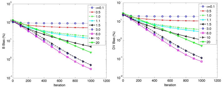
Plots of bias vs. iteration for B (left) and DV (right) parameters for a wide range of lower bounds in the proposed AB-EM algorithm. The results are shown for the putamen in the idealized imaging scenario (in all scenarios, mean B values, as averaged over multiple noise realizations, consistently overestimated the true B values, while mean DV values underestimated the true DV values; nonetheless, for an individual noise realization, towards convergence, both overestimation or underestimation could be observed, as seen in Fig. 3).
Figure 4.
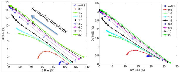
Plots of noise vs. bias for B (left) and DV (right) parameters generated by increasing the number of iterations for a wide range of lower bounds in the proposed AB-EM algorithm. The results are shown for the putamen in the idealized imaging scenario.
At the same time, the parametric image Btrue is not known in practice, and the lower bounds need to be somehow determined. Our approach consisted of initializing the parametric slope DVold and intercept Bold images (in Eq. (9–10)) using parameters DVest and Best as estimated by conventional (indirect) kinetic analysis of dynamic images obtained after a particular number of iterative image updates. Then, to set the vector of spatially-varying lower bounds a, we alternatively defined α such that a=αBest (also recalling that the lower bound was set to 0 for the slope parameter). If Best happened to be positive due to presence of noise, a lower bound of 0 was instead selected (i.e. a=α min(Best,0)). This approach was similarly applied to the reference tissue model. Optimization of the lower bound a and the IUN is presented in Sec. 4.2.3.
2.2. Additional corrections
It is also possible to incorporate corrections for normalization, attenuation, randoms and scatter terms within the proposed 4D-EM framework. Decomposing the system matrix as P=ANG where G denotes the geometric component, and the diagonal matrices A and N represent the attenuation and normalization factors, respectively, (9–11) can then take the following form:
| (14) |
| (15) |
where 1 is a vector of all ones, and
| (16) |
The system matrix can be further modified to incorporate resolution modeling, including the effects of inter-crystal scattering and penetration and/or positron range (e.g. see (Reader et al., 2002; Panin et al., 2006; Rahmim et al., 2008b)), though not explored in this work.
To model randoms and scatter contributions, a straightforward approach is to do so very similar to the conventional ordinary Poisson (OP) EM algorithm by modifying (16) to:
| (17) |
where Rn and Sn represent the total randoms and scatter contributions in each cumulated dataset gn, which can be estimated based on conventional analysis of individual dynamic frames (with each frame corrected for frame-dependent decay and deadtime effects) followed by summation for a given cumulated frame n.
3. Experimental design
3.1. Simulations
A 2-tissue compartmental model was used to simulate dynamic PET studies with reversible binding. For a given plasma input curve Cp(t), as well as nondisplaceable (free+non-specifically-bound) CND(t) and specifically-bound CB(t) compartments, as seen in figure 1, and the four standard rate parameters K1 (ml/min/g), k2 (1/min), k3 (1/min) and k4 (1/min), the kinetics are described by:
| (18) |
| (19) |
Denoting Vp (ml/g) as the fractional plasma volume in tissue, the measured total radioactivity C(t) is given by:
| (20) |
Solution of (18) and (19), and combination with (20), yields the following expression:
| (21) |
where * denotes the convolution operation, and
| (22) |
We emphasize that the abovementioned equations are included to accurately simulate a two-tissue compartment model based on individual rate parameters, while the graphical models (2) and (12) aim to estimate DV and DVR values, as opposed to individual rate parameters, in order to provide more robust estimates.
For our simulations, we made use of 55 11C-raclopride dynamic PET human scans, from which mean K1, k2, k3 and k4 rate constants were generated for multiple regions across the brain. The four kinetic parameters were estimated by fitting the two-tissue compartment model to the measured region-of-interest (ROI) time-activity-curves (TACs) with the ratio K1/k2 constrained to the DV of the cerebellum (reference tissue) for target ROIs. The Marquardt algorithm (Marquardt, 1963) was used for nonlinear fitting with VP fixed at 0.03.
We then used Eq. (21) to simulate the brain kinetics for each region, and subsequently created a set of dynamic images making use of a mathematical brain phantom (Rahmim et al., 2008a) and an acquisition protocol of 4×15 sec, 4×30 sec, 3×1 min, 2×2 min, 5×4 min and 7×5 min. We then performed analytic simulations of all frames to generate dynamic datasets, including multiple realistic noise realizations, followed by reconstruction. Times t in Eq. (2) used for both indirect and direct parametric estimation were 45 min, 50 min, 55 min, 60 min and 65 min, while integrating from t=0; i.e. utilizing all data from 0–65 min.
3.1.1. Idealized imaging
At first, a much simplified simulation scenario was considered, wherein 1-to-1 mapping between image voxels and projection bins was considered: by initially omitting the tomographic reconstruction problem itself (i.e. setting the system matrix Pij=δij), we sought to quantify the ability of the proposed AB-EM algorithm (9–11) to separate slope (DV) and intercept (B) contributions in (2). This approach provided an effective initial study to better understand and quantify convergence, noise and bias properties, given different lower bounds in the AB-EM algorithm (100 noise realizations were simulated and up to 1000 iterative updates were applied to each noise realization).
3.1.2. Tomographic imaging
Subsequently, we performed analytic PET simulations for the geometry of the Discovery RX PET/CT scanner (Kemp et al., 2006), except with the transaxial dimensions (crystal dimensions and field of view) scaled by 0.5 to simulate a dedicated brain scanner. Decay, normalization and attenuation effects were taken into account, while these simulations did not include deadtime, randoms or scattered events (by contrast, the patient study in Sec. 3.2 included additional presence of, and corrections for deadtime, randoms and scattered events).
The data were reconstructed for up to 210 updates (10 iterations; 21 subsets) for both the plasma input and reference tissue models. For the latter, TACs for the cerebellum obtained using conventional reconstruction were used as reference. Indirect parametric imaging was performed by integrating frames first followed by reconstruction (at the same time, this was carefully validated to give very similar quantitative (though more efficient) performance compared to the common approach of reconstructing individual frames followed by integration of images). The indirect approach was then compared with the proposed direct 4D methods for both the plasma input and reference tissue models (25 noise realization were simulated).
3.1.3. Figures of Merit (FOMs)
We studied eleven ROIs, namely the cerebellum, caudate, putamen, cingulate Cx (cortex), occipital Cx, orbitofrontal Cx, parietal Cx, frontal Cx, temporal Cx, thalamus and brain stem (with volumes of 211, 16.5, 5.95, 25.5, 176, 334, 38.1, 190, 204, 22.2 and 41.7 cc, respectively). For reconstructions using multiple noise realizations, the normalized standard deviation (NSDROI) for each ROI was defined as:
| (23) |
where is the DV or DVR parametric value at a voxel j (j=1…MROI) of the specified ROI at noise realization n (n=1…N), and is the ensemble mean value in voxel j, and is the overall mean ROI value.
Next, the regional bias (BiasROI) for a given ROI of known uniform parametric value was defined as:
| (24) |
Furthermore, denoting as the mean regional DV or DVR value for a given noise realization n, the standard deviation (STDROI) of these values across multiple noise realizations was included as an alternative definition of noise:
| (25) |
with the coefficient of variation (COVROI) given by:
| (26) |
The difference between (23) and (26) is that the former first quantifies variations of a given voxel intensity across different noise realizations, followed by averaging across each ROI, while the latter first averages the parameter of interest across each ROI followed by measurement of variation.
Overall FOMs
To quantify NSDoverall as well as COVoverall against Biasoverall for the entire image (in order to allow an overall assessment of quantitative performance), NSDROI, COVROI and BiasROI values for the ROIs (r=1…R) were averaged, weighted by the size (number of voxels MROI) for each ROI.
3.2. Application to patient study
We considered application of the proposed method on the second generation high resolution research tomograph (HRRT) (Sossi et al., 2005). We modified the existing HRRT reconstruction code to enable both: (i) standard kinetic modeling after each iteration through independent reconstruction of the dynamic frames (conventional method) as well as (ii) the proposed 4D direct parametric image reconstruction. In addition to corrections for attenuation and normalization, corrections for randoms and scatter events were also performed (see Sec. 2.2). The randoms and scatter contributions to each data frame were estimated using the singles rate method and the standard single scatter simulation, respectively, for the HRRT scanner (Rahmim et al., 2005).
A 11C- raclopride PET study on a 29 year-old male subject was considered. The reference tissue model (Sec. 2.1.3) was applied for 0–60 min, while four end-times t (45, 50, 55 and 60 min) were considered in (12). The cerebellum TACs were used as reference and were estimated using conventional OSEM reconstructions. Up to fifteen iterations (16 subsets each) of both conventional indirect and proposed 4D direct methods were studied. As also described in Sec. 3.1.2, indirect parametric imaging was performed by integrating frames first followed by reconstruction (though validated to give very similar quantitative performance compared to the common approach of reconstructing individual frames followed by integration of images).
FOMs
Since the true DVR values are not known, BiasROI could not be quantified as was done above for simulations. Furthermore, NSDROI and COVROI as defined above for multiple noise realizations were not invoked. Instead, we plotted NoiseROI vs. DVRROI for a variety of ROIs (each delineated using co-registered MRI image), where NoiseROI was defined as the spatial variation of voxel intensities within each ROI. This approach would allow one to compare noise performance for indirect vs. direct methods, given similarly obtained values of DVR.
4. Results
4.1. Idealized simulation
As discussed in Sec. 3.1.1, a simplified imaging scenario involving 1-to-1 mapping between image voxels and projection data was first considered. This provided an effective initial scheme for preliminary study of the properties of the proposed AB-EM algorithm in its ability to separate slope (DV) and intercept (B) contributions in (2). In particular, the figures below depict simulations for the putamen (Btrue=−40.0 and DVtrue=1.4) where we imposed a wide of range of lower bounds in the AB-EM reconstruction algorithm (10). Defining the fractional parameter α such that the lower bound a was set as a=αBtrue, figure 2 depcits convergence properties for a range of α values. It is seen that for α values below 1 (i.e. the negative lower bound a being closer to zero than Btrue), the algorithm converges (plateaus) to incorrect values. When α is close to one, the convergence was seen to be very slow towards the correct values. By analogy, this is similar to the slow convergence rates observed (Erlandsson et al., 2000; Verhaeghe and Reader, 2010) in standard AB-EM applications for a cold region if the lower bound is set to 0 or only slightly negative. By contrast, there are alternative α values (~6) where convergence is considerably enhanced. Setting α to too high was also seen to slow down the convergence rates. This is attributed to the fact that while the AB-EM algorithm can be shown to converge to the true solution in the noise free case (Byrne, 1998), in the presence of noise, it is in reality an approximation to the EM algorithm, wherein it is assumed that it is the data adjusted by projections of the bounds that are Poisson distributed (i.e. y-Pa in (6) or in (9–10)), and therefore using a lower bound of substantially large magnitude can exhibit adverse convergence properties.
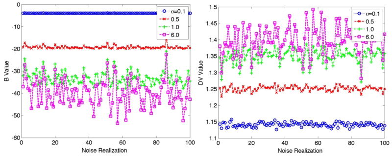
To better comprehend the results in figure 2, figure 3 depicts plots of B and DV values for the individual 100 noise realizations (after 1000 iterative updates). Given Btrue=−40.0 and α values of 0.1 and 0.5 (i.e. lower bounds a of −4.0 and −20.0, respectively), it is seen that the B estimates have converged towards the lower bounds, as they are not able to further approach Btrue. This bias in the B estimates in turns translates itself into biases in the DV estimates in order to compensate for the observed mismatch for B values. Furthermore, we see that as the lower bound further decreases, the bias is reduced but noise levels increase, as also observed in previous studies on 3D reconstruction (Erlandsson et al., 2000; Verhaeghe and Reader, 2010).
Figure 3.
Estimated B (left) and DV (right) values for 100 noise realizations for the putamen. True values for B and DV were −40.0 and 1.4, respectively. The results are shown after 1000 iterations for the putamen. Clear bias is observed for α values below 1 (i.e. when the lower bound a for B is smaller in magnitude compared to the true B value), while the noise is at the same time suppressed.
Figure 4 depicts noise vs. bias plots for the wide range of α values. It is seen, consistent with above figure, that for α values of 0.1 and 0.5, the noise levels are considerably low, but this is at the expense of bias levels stagnating, and not further improving, after some iterations. For α values increasing from 1 onwards it is seen that noise vs. bias performance is further degraded. This is because even though convergence is improved with increasing α values (figure 2), noise levels are also further amplified, and subsequently, noise vs. bias performance is actually seen to degrade (ultimately, the criteria to use for optimization is task-based, and can vary, as discussed in Sec. 5.2).
Furthermore, we note that both bias and noise levels in figure 4 are substantially lower, percentage-wise, for the slope parameter compared to the intercept parameter (as seen by comparing the scale of the axes): this is a favourable property because it is the slope parameter that is of direct interest in parametric imaging.
Finally, we note that the abovementioned studies depict that for optimum performance one must use a general AB-EM formulation wherein the lower bounds are spatially variant and in tune with the values of the intercept parameter at each given position (this is further discussed in Sec. 4.2.3).
4.2. Tomographic simulation
As discussed in Sec. 3.1.2, we also performed extensive PET simulation studies. It was found (see Sec. 2.1.4) that two factors contributed significantly to 4D algorithm performance: initialization (using standard EM followed by modelling at a particular iteration) as well as how the lower bound a was set. We elaborate upon the optimization in Sec. 4.2.3. Below we first discuss comparison of standard indirect versus proposed 4D direct methods when applied to the plasma input (Sec. 4.2.1) and reference tissue (Sec. 4.2.2) models.
4.2.1. Results for the plasma input model
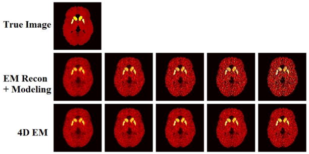
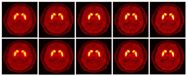
Figure 5 shows typical reconstructed images for indirect and proposed direct parametric imaging methods, with increasing EM iterations from left to right. It is seen that while the standard EM approach results in noisy images, this trend is more controlled and qualitatively improved for the proposed 4D method.
Figure 5.
Estimated parametric DV images. (From left to right): Increasing EM iterations of 1, 2, 3, 5 and 10 (21 subsets). No post-filtering was applied to the images shown.
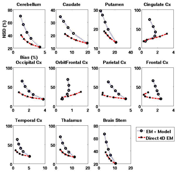
To provide quantitative analysis, figure 6 depicts plots of overall NSD vs. overall bias (as defined in Sec. 3.1.3) for the various parametric DV images shown in figure 5. In addition, figure 7 plots NSDROI vs. BiasROI for 11 individual regions of the brain (cerebellum, caudate, putamen, cingulate Cx (cortex), occipital Cx, orbitofrontal Cx, parietal Cx, frontal Cx, temporal Cx, thalamus and brain stem). It is clearly seen that the proposed direct 4D EM reconstruction results in substantial quantitative accuracy improvements.
Figure 6.
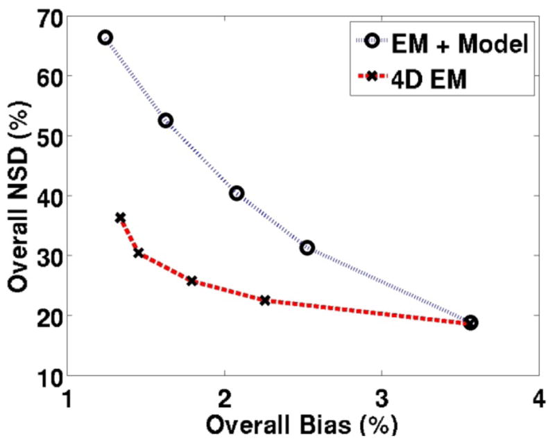
Plots of overall NSD (noise) vs. overall bias comparing parametric DV images obtained from standard indirect method (EM reconstruction followed by modeling) as well as the proposed direct 4D technique. The plasma input model was used. Points on each curve (right to left) correspond to the images of increasing iterations in each row of figure 5.
Figure 7.
Plots of NSDROI (noise) vs. BiasROI for DV images obtained using standard EM and the proposed direct 4D EM technique (plasma input model). Points on each curve correspond to the images in each row of figure 5. The actual DV values for the 11 regions (cerebellum to brain stem, in the order shown) were 0.298, 1.151, 1.398, 0.364, 0.365, 0.351, 0.359, 0.328, 0.377, 0.443 and 0.403, respectively (this implies DVR values of 1, 3.865, 4.694, 1.222, 1.226, 1.179, 1.206, 1.102, 1.264, 1.488 and 1.3517, respectively). Also, the actual intercept B values were −0.973, −29.80, −40.37, −2.34, −3.04, −2.14, −2.83, −1.62, −2.76, −2.62 and −5.98 for the plasma input model, and for the reference tissue model θ, they were 0, −76.98, −105.8, −3.39, −5.47, −2.92, −4.90, −1.60, −4.52, −3.47 and −13.77, respectively.
As also discussed in Sec. 3.1.3, we also performed analysis of COV (as an alternative measure of noise) vs. bias. The trade-off curves shown in figure 8 for the estimated DV parametric images demonstrate substantial quantitative improvements for the proposed method, as also demonstrated in figure 6 (trade-off curves for individual regions, not shown, also showed similar improvements). The scale of COV values in figure 8 are smaller than NSD values in figure 6, because COV analysis calculates standard deviation of ROIs averaged values across multiple noise realization which are much less sensitive to noise than NSD calculation which performs noise analysis for individual voxels, followed by averaging across the ROIs (see discussion following Eq. (26)).
Figure 8.
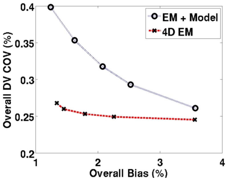
Plots of overall COV (alternative measure of noise) vs. bias comparing parametric DV images obtained from standard indirect method as well as the proposed direct 4D technique. The plasma input model was used.
We also wish to note that in actual patient test-retest studies, issues of variability in radiotracer uptake as well as ROI delineation between patient scans further degrade reproducibility in parametric estimates (not simulated here). Moreoever, we note that ROI definitions in the present simulations, based on the known true images, extended across the entirety of each region. By using smaller ROI definitions (avoiding the edges), estimated COV values were seen to further increase, though similar overall performances were observed.
4.2.2. Results for the reference tissue model
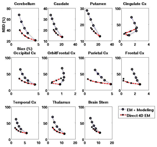
The abovementioned quantitative analysis was also performed on parametric DVR images obtained using the reference tissue model (Sec. 2.1.2), with the cerebellum used as reference. For DVR images obtained using indirect and proposed direct methods, figure 9 shows NSDROI vs. BiasROI as generated using increasing iterations, demonstrating quantitative improvements for the direct 4D method (similar to the results for the plasma input model in figures 6 and 7). Furthermore, as in figure 8, COV vs. Bias plots were also seen to depict quantitative improvements in noise vs. bias performance (not shown). It is worth noting that in conventional imaging, variability of DVR (and therefore BPND=DVR−1) estimates is too high for the relatively low uptake BPND regions of cortical grey and thalamus, and are typically not reliable. The proposed approach is thus seen to increase feasibility of imaging low BPND images.
Figure 9.
Regional noise (NSD) vs. bias (RB) curves for DVR images obtained using standard EM vs. proposed direct 4D EM technique (reference tissue model with cerebellum used as reference). Actual DVR values are mentioned in the caption for figure 7.
4.2.3. Parameter optimization for the direct 4D method
As discussed in Sec. 2.1.4, image initialization as well as definition of the lower bound vector a noticeably impacted algorithm performance. We utilized an approach wherein initial estimates of the slope DVest and intercept Best parameters were obtained by conventional parametric imaging, as applied to dynamic images obtained after a certain number of iterations: this number is referred to as the initialized update number (IUN); for instance IUN=21 indicates that the initial estimates were obtained using kinetic analysis of dynamic images reconstructed after 21 updates (which happens to be a full iteration because each iteration consists of 21 subsets). Furthermore, as mentioned in Sec. 2.1.4, to set the lower bound a, we defined α such that a= α min(Best,0)).
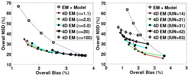
Figure 10 depicts quantitative performance for the plasma input model for a range of (left) α and (right) IUN values. In the plots at (left), similar to figure 4, it was seen that optimum noise vs. bias performance was obtained using α values close to 1 (though, setting α exactly equal to 1 was avoided to prevent stagnation of updates in Eq. (9): this is because for negative Best values, if α=1 then Bold−a= Best−a=0 in (9) and thus B values do not subsequently update; by analogy, this is equivalent to initializing image estimates in the standard EM algorithm to zero, which would then fail to change in subsequent updates).
Figure 10.
Regional NSD (noise) vs. bias curves for DV images obtained using standard EM and the proposed direct 4D EM technique for varying (left) lower bounds (fixing IUN=21) and (right) IUN values (fixing α=1.1).
In figure 10 (right), IUN optimization by comparing the various 4D EM trade-off curves was less straightforward, and IUN=21 was ultimately selected as optimum; nonetheless one sees that all initializations shown outperformed the conventional scheme. At the same time, we observed that setting IUN to smaller values resulted in sub-optimal trade-off performance curves (not shown).
4.3. Application to HRRT patient study
We then applied the proposed reference tissue model to a 11C- raclopride patient study on the HRRT scanner (elaborated in Sec. 3.2). To provide a visual/qualitative comparison, figure 11 plots images of increasing iterations for the conventional indirect as well as proposed 4D direct parametric imaging techniques, depicting relatively reduced noise levels as a function of iteration.
Figure 11.
Parametric DVR images for a raclopride HRRT study with increasing iterations of 2, 3, 4, 7, 15 from left to right. (Top) Standard 3D reconstruction followed by modeling; (bottom) Proposed 4D reconstruction (reference tissue model). The images include no post-smoothing. Images are shown on the same color scale.
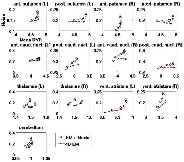
To additionally compare the images quantitatively (see Sec. 3.2), figure 12 depicts NoiseROI vs. DVRROI plots generated by increasing iterations, for thirteen regions of: cerebellum as well as both left (L) and right (R) anterior putamen, posterior putamen, anterior caudate nucleus, posterior caudate nucleus, thalamus and ventral striatum. Across these ROIs, the proposed 4D method is seen to generally outperform the conventional method in the sense that for a given DVR value, improved noise levels are observed.
Figure 12.
Noise vs. DVR curves (generated by increasing iterations as seen in figure 11), comparing performance of conventional indirect vs. direct 4D estimated DVR images.
Our future work consists of application to a large pool of patients scanned on the HRRT scanner: we will explore whether the proposed direct 4D AB-EM reconstruction will produce parameter estimates with enhanced quantitative accuracy, including enhanced separability between patients vs. healthy control subjects, as well as improved consistency within healthy controls.
5. Discussion
5.1. Sign-constraint considerations
In order to address the challenge of the intercept parameters being commonly negative in reversible binding graphical analysis (Sec. 2.1.1), our initial preliminary work (Rahmim et al., 2009b) instead proposed the following approach: Eq. (2) can be subtracted by its own counterpart where time t is replaced by an earlier time t0 (at which the RE condition is also valid) to yield:
| (27) |
Now, defining:
| (28) |
and given that at late times t>t0 (away from the initial uptake phase), the plasma input function tends to decrease as a function of time, i.e. ΔCp (t, t0) < 0, one may re-write (27) as:
| (29) |
Now, both terms in the brackets are non-negative, and as such, the 4D EM algorithm (without the AB modification) can be applied to this equation. In fact, the time-limited RE formulation (27), or its Logan counterpart, may at first suggest the possibility to not require scanning the subjects at early times prior to t0. However, an important observation is that (27) is only equivalent to (2) in the ideal noise-free scenario, and that in fact it can perform very poorly in the presence of noise, as it neglects data prior to t0. This is depicted in figure 13 wherein application of indirect kinetic analysis to the subject HRRT PET data (Sec. 3.2) using models (2) vs. (27) demonstrated vivid quantitative degradations for the latter.
Figure 13.
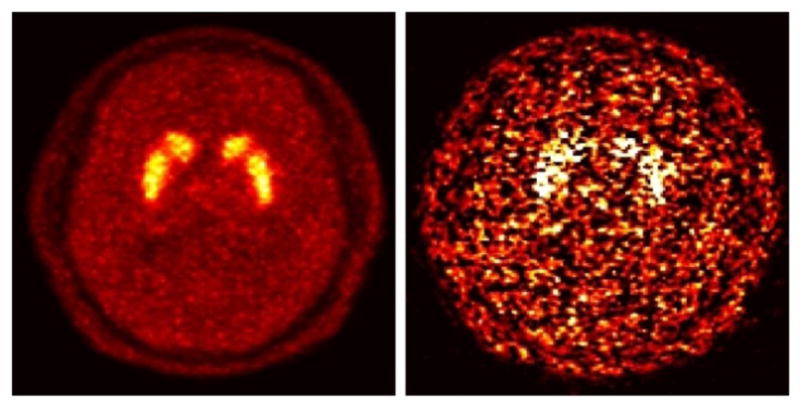
Parametric DVR images for the raclopride HRRT study (Sec. 3.2) estimated using graphical kinetic analysis based on (left) Eq. (2) vs. (right) Eq. (27) where in the latter t0 was set to 40 min.
By contrast, the 4D AB-EM technique formulated in the present work, as elaborated in Sec. 2, provides an effective solution to the abovementioned sign-constraint consideration, and has been shown to outperform indirect parametric imaging involving the more appropriate formulation (2) wherein the entire dataset is considered.
5.2. Quantitative analysis methods
Convergence rates (as studied in figures 2 and 3) may be used as a quantitative criterion for algorithm optimization and evaluation. At the same time, the techniques studies in the present work were primarily optimized and evaluated using quantitative dual-metric noise vs. bias trade-off curve analysis (figures 4–10). We prefer the latter because of additional consideration of noise properties. Some authors (e.g. (Verhaeghe and Reader, 2010)) have instead utilized the root mean square error (RMSE), a single metric that essentially combines, and equally weights, the noise and bias metrics. Nonetheless, it is important to note that, ultimately, image quality optimization and assessment is best performed in the context of the particular task of interest (Barrett and Myers, 2004), e.g. (a) lesion detection, (b) lesion discrimination (e.g. whether a tumor is cystic or has a necrotic center), or (c) quantification of BPND differences between subject populations in particular ROIs. As such, unequal emphases on noise vs. bias metrics may be imposed depending on task (e.g. lesion detection tasks tend to prefer lower noise levels compared to discrimination tasks (Tsui et al., 1983; Tsui, 1978)). In fact, dual metric noise vs. bias analysis can be viewed as a robust and reliable initial validation phase towards task-based assessment of image quality (Lee and Tsui, 2009a, b) having the ability to narrow down the range of parameters to be studied in subsequent observer studies.
5.3. Applicability to different tracers
The RE formulation (2) is applicable to tracers with reversible binding which attain relative equilibrium with respect to the plasma input at a time t≥ t* within the scan period. This includes tracers such as [11C]PIB (Zhou et al., 2009a) and [11C]raclopride (Zhou et al., 2009b). At the same time, a number of other tracers (e.g. [11C]WIN35,428 and 10 [11C]MDL100,907) do not follow such kinetics. In (Zhou et al., 2010), it was shown that another linear formulation is still possible, namely by decomposing the problem into two components: (1) the RE component as estimated using the abovementioned RE formulation, and (2) the non-RE component that can be estimated by the Patlak linear model. In fact, the Patlak model has already been incorporated within direct 4D parameter estimation (Wang et al., 2008; Tsoumpas et al., 2008a; Tang et al., 2010). It is therefore possible, as we shall investigate, to combine the abovementioned RE and Patlak 4D parametric imaging algorithms to arrive at a more general and comprehensive 4D model applicable to a wide range of tracers.
5.4. Other issues
Reference tissue TAC estimation
We wish to note that the TAC of the reference tissue (cerebellum) as incorporated within our proposed direct parametric imaging is itself obtained using an initial reconstruction, and as such, may be affected by limitations of conventional reconstruction (nonnegligible bias and noise). At the same time, we emphasize that: (i) by utilizing a large ROI in the cerebellum, as we have done, the effect of noise can be significantly reduced. Furthermore, (ii) the effect of bias in the reference tissue TAC impacts both conventional and proposed reconstruction methods, and as we clearly observe in this work, the proposed method, given its comprehensive 4D imaging model, still results in enhanced quantitative performance. At the same time, it is plausible that the use of methods that simultaneously estimate the input function and kinetic parameters within a 4D framework (Reader et al., 2007) could lead to further enhanced performance.
Weighting
Parameter estimation in indirect kinetic analysis of PET data, as implemented in our work, did not include weighted regression, as was also the case in the original work by Zhou et al. (2009b). This is because unlike non-linear kinetic modeling methods which include widely varying statistics amongst the image sets being analyzed, the present analysis is in the domain of linear graphical modeling and only involves cumulated frames with end times in the 40–65 min range and a start time of t=0 (thus having very similar statistics). As such, additional inclusion of weighting does not noticeably impact performance.
Motion
Subject motion in brain PET is an important factor contributing to deterioration of image quality and quantitative accuracy, as a result of which a wide range of motion correction methods have been developed (e.g. see review (Rahmim et al., 2007)). 4D techniques, while providing a powerful framework for dynamic PET image reconstruction, are challenged by an enhanced sensitivity to subject motion (Verhaeghe et al., 2010). In addition, application of motion compensation to 4D methods is less straight-forward: for instance, a very simple and relatively common approach in conventional reconstruction is to realign post-reconstructed images to a particular frame used as reference. In direct parametric imaging, however, it is the parametric image and not the individual dynamic frames that are directly reconstructed. In 4D reconstruction, a potential alternative to above motion correction method is to first estimate inter-frame movements via registration of preliminary reconstructions based on the conventional scheme, followed by transformation of the projection data in each frame to account for the estimated motion, followed by 4D reconstruction. Alternatively, one may utilize external tracking motion information to perform such correction on the collective frame data, or even individual lines-of-response (LORs), followed by 4D reconstruction. Nonetheless, it has been shown that mere transformation of projections is not sufficient to achieve reliable motion compensation and must be accompanied by additional modeling of probabilities of detection being modified due to presence of motion (Qi and Huesman, 2002; Carson et al., 2003; Rahmim et al., 2004; Buhler et al., 2004). Such an approach was in fact recently developed and studied in the context of 4D reconstruction, involving the generation of normalization files specific to each data frame to account for modified probabilities of detection due to motion (Verhaeghe et al., 2010). The 4D AB-EM algorithm proposed in the present work may also be modified accordingly to enable motion compensation.
6. Summary
This work proposed a closed-form iterative 4D EM algorithm, involving generalization of the AB-EM algorithm to the 4D domain, which was applied to both plasma input and reference tissue models in the context of reversible binding PET imaging. The technique thus moved beyond the conventional approach of independent-frame reconstruction of dynamic datasets followed by modeling, and was shown to result in quantitatively enhanced DV and DVR parametric images, as demonstrated in extensive 11C-raclopride PET simulations as well as an HRRT patient study.
Acknowledgments
This work was in part supported by the NIH grants 1S10RR023623, DA00412, MH078175 and AA12839. The authors also wish to thank Andrew Crabb for computational support, and Hiroto Kuwabara and Anil Kumar for help with delineation of ROIs in patient study.
References
- Abi-Dargham A, Martinez D, Mawlawi O, Simpson N, Hwang DR, Slifstein M, Anjilvel S, Pidcock J, Guo NN, Lombardo I, Mann JJ, Van Heertum R, Foged C, Halldin C, Laruelle M. Measurement of striatal and extrastriatal dopamine D1 receptor binding potential with [11C]NNC 112 in humans: validation and reproducibility. J Cereb Blood Flow Metab. 2000;20:225–43. doi: 10.1097/00004647-200002000-00003. [DOI] [PubMed] [Google Scholar]
- Barrett HH, Myers KJ. Foundations of Image Science. Hoboken, New Jersey: Wiley & Sons, Inc; 2004. [Google Scholar]
- Bentourkia M, Zaidi H. Tracer kinetic modeling in PET. PET Clinics. 2007;2:267–77. doi: 10.1016/j.cpet.2007.08.003. [DOI] [PubMed] [Google Scholar]
- Buhler P, Just U, Will E, Kotzerke J, van den Hoff J. An accurate method for correction of head movement in PET. IEEE Trans Med Imaging. 2004;23:1176–85. doi: 10.1109/TMI.2004.831214. [DOI] [PubMed] [Google Scholar]
- Byrne C. Iterative algorithms for deblurring and deconvolution with constraints. Inverse Problems. 1998;14:1455–67. [Google Scholar]
- Carson RE, Barker WC, Liow J-S, Johnson CA. Design of a motion-compensation OSEM list-mode algorithm for resolution-recovery reconstruction for the HRRT. IEEE Nuclear Science Symposium Conference Record; 19–25 October 2003; Portland; OR; USA. 2003. pp. 3281–5. [Google Scholar]
- Carson RE, Lange K. The EM parametric image reconstruction algorithm. J Am Statist Assoc. 1985;80:20–2. [Google Scholar]
- Chiao P-C, Rogers WL, Clinthorne NH, Fessler JA, Hero AO. Model-based estimation for dynamic cardiac studies using ECT. Medical Imaging, IEEE Transactions on. 1994;13:217–26. doi: 10.1109/42.293914. [DOI] [PubMed] [Google Scholar]
- Erlandsson K, Visvikis D, Waddington WA, Cullum I, Jarritt PH, Polowsky LS. Low-statistics reconstruction with AB-EMML. Nuclear Science Symposium Conference Record; 2000; IEEE. 2000. pp. 15/249–15/53. [Google Scholar]
- Fujimura Y, Ikoma Y, Yasuno F, Suhara T, Ota M, Matsumoto R, Nozaki S, Takano A, Kosaka J, Zhang MR, Nakao R, Suzuki K, Kato N, Ito H. Quantitative analyses of 18F-FEDAA1106 binding to peripheral benzodiazepine receptors in living human brain. J Nucl Med. 2006;47:43–50. [PubMed] [Google Scholar]
- Gunn RN, Gunn SR, Turkheimer FE, Aston JA, Cunningham VJ. Positron emission tomography compartmental models: a basis pursuit strategy for kinetic modeling. J Cereb Blood Flow Metab. 2002;22:1425–39. doi: 10.1097/01.wcb.0000045042.03034.42. [DOI] [PubMed] [Google Scholar]
- Innis RB, Cunningham VJ, Delforge J, Fujita M, Giedde A, Gunn RN, Holden J, Houle S, Huang SC, Ichise M, Lida H, Ito H, Kimura Y, Koeppe RA, Knudsen GM, Knuuti J, Lammertsma AA, Laruelle M, Logan J, Maguire RP, Mintun MA, Morris ED, Parsey R, Price JC, Slifstein M, Sossi V, Suhara T, Votaw JR, Wong DF, Carson RE. Consensus nomenclature for in vivo imaging of reversibly binding radioligands. Journal of Cerebral Blood Flow and Metabolism. 2007;27:1533–9. doi: 10.1038/sj.jcbfm.9600493. [DOI] [PubMed] [Google Scholar]
- Kadrmas DJ, Gullberg GT. 4D maximum a posteriori reconstruction in dynamic SPECT using a compartmental model-based prior. Phys Med Biol. 2001;46:1553–74. doi: 10.1088/0031-9155/46/5/315. [DOI] [PMC free article] [PubMed] [Google Scholar]
- Kamasak ME, Bouman CA, Morris ED, Sauer K. Direct reconstruction of kinetic parameter images from dynamic PET data. IEEE Trans Med Imaging. 2005;24:636–50. doi: 10.1109/TMI.2005.845317. [DOI] [PubMed] [Google Scholar]
- Kemp BJ, Kim C, Williams JJ, Ganin A, Lowe VJ. NEMA NU 2–2001 performance measurements of an LYSO-based PET/CT system in 2D and 3D acquisition modes. J Nucl Med. 2006;47:1960–7. [PubMed] [Google Scholar]
- Lange K, Hunter DR, Yang I. Optimization transfer using surrogate objective functions. J Comput Graph Stat. 2000;9:1–20. [Google Scholar]
- Lee T-S, Segars WP, Tsui BMW. Study of parameters characterizing space-time Gibbs priors for 4D MAP-RBI-EM in gated myocardial perfusion SPECT. Nuclear Science Symposium Conference Record; 2005; IEEE. 2005. pp. 2124–8. [Google Scholar]
- Lee T-S, Tsui BMW. Comparison of Quantitative and Task-Based Optimizations of a 4D MAP-RBI-EM Reconstruction Methods for Gated Myocardial Perfusion SPECT. Nuclear Science Symposium Conference Record; 2009; IEEE. 2009a. [Google Scholar]
- Lee T-S, Tsui BMW. Optimization of a 4D Space-Time Gibbs Prior in a 4D MAP-RBI-EM Reconstruction Method for Application to Gated Myocardial Perfusion SPECT. Fully Three-Dimensional Image Reconstruction Meeting in Radiology and Nuclear Medicine; Beijing, China. 2009b. [Google Scholar]
- Li Q, Asma E, Ahn S, Leahy RM. A fast fully 4-D incremental gradient reconstruction algorithm for list mode PET data. IEEE Trans Med Imaging. 2007;26:58–67. doi: 10.1109/TMI.2006.884208. [DOI] [PubMed] [Google Scholar]
- Logan J. Graphical analysis of PET data applied to reversible and irreversible tracers. Nucl Med Biol. 2000;27:661–70. doi: 10.1016/s0969-8051(00)00137-2. [DOI] [PubMed] [Google Scholar]
- Logan J, Fowler JS, Volkow ND, Ding YS, Wang GJ, Alexoff DL. A strategy for removing the bias in the graphical analysis method. J Cereb Blood Flow Metab. 2001;21:307–20. doi: 10.1097/00004647-200103000-00014. [DOI] [PubMed] [Google Scholar]
- Logan J, Fowler JS, Volkow ND, Wolf AP, Dewey SL, Schlyer DJ, MacGregor RR, Hitzemann R, Bendriem B, Gatley SJ, et al. Graphical analysis of reversible radioligand binding from time-activity measurements applied to [N-11C-methyl]-(−)-cocaine PET studies in human subjects. J Cereb Blood Flow Metab. 1990;10:740–7. doi: 10.1038/jcbfm.1990.127. [DOI] [PubMed] [Google Scholar]
- Marquardt DW. An Algorithm for Least-Squares Estimation of Nonlinear Parameters. Journal of the Society for Industrial and Applied Mathematics. 1963;11:431–41. [Google Scholar]
- Matthews J, Bailey D, Price P, Cunningham V. The direct calculation of parametric images from dynamic PET data using maximum-likelihood iterative reconstruction. Phys Med Biol. 1997;42:1155–73. doi: 10.1088/0031-9155/42/6/012. [DOI] [PubMed] [Google Scholar]
- Meikle SR, Matthews JC, Cunningham VJ, Bailey DL, Livieratos L, Jones T, Price P. Parametric image reconstruction using spectral analysis of PET projection data. Phys Med Biol. 1998;43:651–66. doi: 10.1088/0031-9155/43/3/016. [DOI] [PubMed] [Google Scholar]
- Narayanan MV, King MA, Soares EJ, Byrne CL, Pretorius PH, Wernick MN. Application of the Karhunen-Loeve transform to 4D reconstruction of cardiac gated SPECT images. IEEE Transactions on Nuclear Science. 1999a;46:1001–8. [Google Scholar]
- Narayanan MV, King MA, Soares EJ, Byrne CL, Pretorius PH, Wernick MN. Application of the Karhunen-Loeve transform to 4D reconstruction of cardiac gated SPECT images. IEEE Trans Nuc Sci. 1999b;46:1001–8. [Google Scholar]
- Nichols TE, Qi J, Asma E, Leahy RM. Spatiotemporal reconstruction of list-mode PET data. IEEE Trans Med Imaging. 2002;21:396–404. doi: 10.1109/TMI.2002.1000263. [DOI] [PubMed] [Google Scholar]
- Nuyts J, Stroobants S, Dupont P, Vleugels S, Flamen P, Mortelmans L. Reducing loss of image quality because of the attenuation artifact in uncorrected PET whole-body images. Journal of Nuclear Medicine. 2002;43:1054–62. [PubMed] [Google Scholar]
- Panin VY, Kehren F, Michel C, Casey M. Fully 3-D PET reconstruction with system matrix derived from point source measurements. IEEE Trans Med Imaging. 2006;25:907–21. doi: 10.1109/tmi.2006.876171. [DOI] [PubMed] [Google Scholar]
- Qi JY, Huesman RH. List mode reconstruction for PET with motion compensation: A simulation study. 2002 Ieee International Symposium on Biomedical Imaging, Proceedings; 2002. pp. 413–6. [Google Scholar]
- Rahmim A, Bloomfield P, Houle S, Lenox M, Michel C, Buckley KR, Ruth TJ, Sossi V. Motion compensation in histogram-mode and list-mode EM reconstructions: beyond the event-driven approach. IEEE Trans Nucl Sci. 2004;51:2588–96. [Google Scholar]
- Rahmim A, Cheng JC, Blinder S, Camborde ML, Sossi V. Statistical dynamic image reconstruction in state-of-the-art high-resolution PET. Phys Med Biol. 2005;50:4887–912. doi: 10.1088/0031-9155/50/20/010. [DOI] [PubMed] [Google Scholar]
- Rahmim A, Dinelle K, Cheng JC, Shilov MA, Segars WP, Lidstone SC, Blinder S, Rousset OG, Vajihollahi H, Tsui BM, Wong DF, Sossi V. Accurate event-driven motion compensation in high-resolution PET incorporating scattered and random events. IEEE Trans Med Imaging. 2008a;27:1018–33. doi: 10.1109/TMI.2008.917248. [DOI] [PMC free article] [PubMed] [Google Scholar]
- Rahmim A, Rousset OG, Zaidi H. Strategies for motion tracking and correction in PET. PET Clinics. 2007;2:251–66. doi: 10.1016/j.cpet.2007.08.002. [DOI] [PubMed] [Google Scholar]
- Rahmim A, Tang J, Lodge MA, Lashkari S, Ay MR, Lautamaki R, Tsui BM, Bengel FM. Analytic system matrix resolution modeling in PET: an application to Rb-82 cardiac imaging. Phys Med Biol. 2008b;53:5947–65. doi: 10.1088/0031-9155/53/21/004. [DOI] [PMC free article] [PubMed] [Google Scholar]
- Rahmim A, Tang J, Muhy-ud-Din H, Ay MR, Lodge MA. Use of optimization transfer for enhanced direct 4D parametric imaging in myocardial perfusion PET. J Nuc Med. 2011;51(suppl 1):265. [Google Scholar]
- Rahmim A, Tang J, Zaidi H. Four-dimensional (4-D) image reconstruction strategies in dynamic PET: beyond conventional independent frame reconstruction. Med Phys. 2009a;36:3654–70. doi: 10.1118/1.3160108. [DOI] [PubMed] [Google Scholar]
- Rahmim A, Zaidi H. PET versus SPECT: strengths, limitations and challenges. Nucl Med Commun. 2008;29:193–207. doi: 10.1097/MNM.0b013e3282f3a515. [DOI] [PubMed] [Google Scholar]
- Rahmim A, Zhou Y, Tang J, Wong DF. Direct 4D parametric image reconstruction with plasma input and reference tissue models in reversible binding imaging. IEEE Nucl Sci Symp Conf Record. 2009b:2516–22. [Google Scholar]
- Reader AJ, Ally S, Bakatselos F, Manavaki R, Walledge RJ, Jeavons AP, Julyan PJ, Zhao S, Hastings DL, Zweit J. One-pass list-mode EM algorithm for high-resolution 3-D PET image reconstruction into large arrays. IEEE Trans Nuc Sci. 2002;49:693–9. [Google Scholar]
- Reader AJ, Matthews JC, Sureau FC, Comtat C, Trebossen R, Buvat I. Iterative Kinetic Parameter Estimation within Fully 4D PET Image Reconstruction. Nuclear Science Symposium Conference Record; 2006; IEEE. 2006a. pp. 1752–6. [Google Scholar]
- Reader AJ, Matthews JC, Sureau FC, Comtat C, Trebossen R, Buvat I. Fully 4D image reconstruction by estimation of an input function and spectral coefficients. Nuclear Science Symposium Conference Record, 2007. NSS ’07; IEEE. 2007. pp. 3260–7. [Google Scholar]
- Reader AJ, Sureau F, Comtat C, Trebossen R, Buvat I. Simultaneous Estimation of Temporal Basis Functions and Fully 4D PET Images. Nuclear Science Symposium Conference Record; 2006; IEEE. 2006b. pp. 2219–23. [Google Scholar]
- Reader AJ, Sureau FC, Comtat C, Trebossen R, Buvat I. Joint estimation of dynamic PET images and temporal basis functions using fully 4D ML-EM. Phys Med Biol. 2006c;51:5455–74. doi: 10.1088/0031-9155/51/21/005. [DOI] [PubMed] [Google Scholar]
- Slifstein M, Laruelle M. Effects of statistical noise on graphic analysis of PET neuroreceptor studies. J Nucl Med. 2000;41:2083–8. [PubMed] [Google Scholar]
- Snyder DL. Parameter Estimation for Dynamic Studies in Emission-Tomography Systems Having List-Mode Data. Nuclear Science, IEEE Transactions on. 1984;31:925–31. [Google Scholar]
- Sossi V, de Jong HWAM, Barker WC, Bloomfield P, Burbar Z, Camborde ML, Comtat C, Eriksson LA, Houle S, Keator D, Knob C, Krais R, Lammertsma AA, Rahmim A, Sibomana M, Teras M, Thompson CJ, Trebossen R, Votaw J, Walker M, Wienhard K, Wong DF. The second generation HRRT - a multi-centre scanner performance investigation. Nuclear Science Symposium Conference Record; 2005; IEEE. 2005. pp. 2195–9. [Google Scholar]
- Tang J, Bengel F, Zhou Y, Valenzuela PB, Rahmim A. Direct 4D parametric image reconstruction for dynamic cardiac PET imaging. J Nuc Med. 2011;51(suppl 1) 1996. [Google Scholar]
- Tang J, Kuwabara H, Wong DF, Rahmim A. Direct 4D reconstruction of parametric images incorporating anato-functional joint entropy. Phys Med Bio. 2010;55:1–12. doi: 10.1088/0031-9155/55/15/005. [DOI] [PMC free article] [PubMed] [Google Scholar]
- Topping GJ, Dinelle K, Kornelsen R, McCormick S, Holden JE, Sossi V. Positron Emission Tomography Kinetic Modeling Algorithms for Small Animal Dopaminergic System Imaging. Synapse (New York, N Y. 2010;64:200–8. doi: 10.1002/syn.20716. [DOI] [PubMed] [Google Scholar]
- Tsoumpas C, Turkheimer FE, Thielemans K. Study of direct and indirect parametric estimation methods of linear models in dynamic positron emission tomography. Med Phys. 2008a;35:1299–309. doi: 10.1118/1.2885369. [DOI] [PubMed] [Google Scholar]
- Tsoumpas C, Turkheimer FE, Thielemans K. A survey of approaches for direct parametric image reconstruction in emission tomography. Med Phys. 2008b;35:3963–71. doi: 10.1118/1.2966349. [DOI] [PubMed] [Google Scholar]
- Tsui BMW. Correction to a Comparison of Optimum Detector Spatial-Resolution in Nuclear Imaging Based on Statistical-Theory and Observer Performance. Physics in Medicine and Biology. 1978;23:1203–5. doi: 10.1088/0031-9155/23/6/421. [DOI] [PubMed] [Google Scholar]
- Tsui BMW, Metz CE, Beck RN. Optimum Detector Spatial-Resolution for Discriminating between Tumor Uptake Distributions in Scintigraphy. Physics in Medicine and Biology. 1983;28:775–88. doi: 10.1088/0031-9155/28/7/001. [DOI] [PubMed] [Google Scholar]
- Verhaeghe J, D’Asseler Y, Vandenberghe S, Staelens S, Lemahieu I. An investigation of temporal regularization techniques for dynamic PET reconstructions using temporal splines. Med Phys. 2007;34:1766–78. doi: 10.1118/1.2723879. [DOI] [PubMed] [Google Scholar]
- Verhaeghe J, Gravel P, Mio R, Fukasawa R, Rosa-Neto P, Soucy JP, Thompson CJ, Reader AJ. Motion compensation for fully 4D PET reconstruction using PET superset data. Physics in Medicine and Biology. 2010;55:4063–82. doi: 10.1088/0031-9155/55/14/008. [DOI] [PubMed] [Google Scholar]
- Verhaeghe J, Reader AJ. AB-OSEM reconstruction for improved Patlak kinetic parameter estimation: a simulation study. Physics in Medicine and Biology. 2010;55:6739–57. doi: 10.1088/0031-9155/55/22/009. [DOI] [PubMed] [Google Scholar]
- Verhaeghe J, Van De Ville D, Khalidov I, D’Asseler Y, Lemahieu I, Unser M. Dynamic PET Reconstruction Using Wavelet Regularization With Adapted Basis Functions. Medical Imaging, IEEE Transactions on. 2008;27:943–59. doi: 10.1109/TMI.2008.923698. [DOI] [PubMed] [Google Scholar]
- Walledge RJ, Manavaki R, Honer M, Reader AJ. Inter-frame filtering for list-mode EM reconstruction in high-resolution 4-D PET. IEEE Trans Nuc Sci. 2004;51:705–11. [Google Scholar]
- Wallius E, Nyman M, Oikonen V, Hietala J, Ruotsalainen U. Voxel-based NK1 receptor occupancy measurements with [(18)F]SPA-RQ and positron emission tomography: a procedure for assessing errors from image reconstruction and physiological modeling. Mol Imaging Biol. 2007;9:284–94. doi: 10.1007/s11307-007-0096-1. [DOI] [PubMed] [Google Scholar]
- Wang G, Fu L, Qi J. Maximum a posteriori reconstruction of the Patlak parametric image from sinograms in dynamic PET. Phys Med Biol. 2008;53:593–604. doi: 10.1088/0031-9155/53/3/006. [DOI] [PubMed] [Google Scholar]
- Wang G, Qi J. Iterative nonlinear least squares algorithms for direct reconstruction of parametric images from dynamic PET. Biomedical Imaging: From Nano to Macro, 2008. ISBI 2008. 5th IEEE International Symposium on; 2008. pp. 1031–4. [Google Scholar]
- Wang G, Qi J. Acceleration of the direct reconstruction of linear parametric images using nested algorithms. Phys Med Biol. 2010;55:1505–17. doi: 10.1088/0031-9155/55/5/016. [DOI] [PMC free article] [PubMed] [Google Scholar]
- Wang GB, Qi JY. Generalized Algorithms for Direct Reconstruction of Parametric Images From Dynamic PET Data. IEEE Trans Med Imaging. 2009;28:1717–26. doi: 10.1109/TMI.2009.2021851. [DOI] [PMC free article] [PubMed] [Google Scholar]
- Wernick MN, Infusino EJ, Milosevic M. Fast spatio-temporal image reconstruction for dynamic PET. IEEE Trans Med Imaging. 1999;18:185–95. doi: 10.1109/42.764885. [DOI] [PubMed] [Google Scholar]
- Yan J, Planeta-Wilson B, Carson RE. Direct 4D list mode parametric reconstruction for PET with a novel EM algorithm. IEEE NSS/MIC Conf. Proceed; 2008. [DOI] [PMC free article] [PubMed] [Google Scholar]
- Zeng GL, Gullberg GT, Huesman RH. Using linear time-invariant system theory to estimate kinetic parameters directly from projection measurements. Nuclear Science, IEEE Transactions on. 1995;42:2339–46. [Google Scholar]
- Zhou Y, Resnick S, Ye W, Sokkova J, Wong DF. Using a consistent graphical analysis method to improve the voxel-wise quantification of [11C]PIB dynamic PET. Jorunal of Nuclear Medicine. 2009a;50:31. [Google Scholar]
- Zhou Y, Ye W, Brasic JR, Crabb AH, Hilton J, Wong DF. A consistent and efficient graphical analysis method to improve the quantification of reversible tracer binding in radioligand receptor dynamic PET studies. Neuroimage. 2009b;44:661–70. doi: 10.1016/j.neuroimage.2008.09.021. [DOI] [PMC free article] [PubMed] [Google Scholar]
- Zhou Y, Ye W, Brasic JR, Wong DF. Multi-graphical analysis of dynamic PET. Neuroimage. 2010;49:2947–57. doi: 10.1016/j.neuroimage.2009.11.028. [DOI] [PMC free article] [PubMed] [Google Scholar]


