

Abstract
The authors examined the relationship of alcohol outlet density (AOD) and neighborhood poverty with binge drinking and alcohol-related problems among drinkers in married and cohabitating relationships and assessed whether these associations differed across sex. A U.S. national population couples survey was linked to U.S. Census data on AOD and neighborhood poverty. The 1,784 current drinkers in the survey reported on their binge drinking, alcohol-related problems, and other covariates. AOD was defined as the number of alcohol outlets per 10,000 persons and was obtained at the zip code level. Neighborhood poverty was as having a low (<20%) or high (≥20%) proportion of residents living in poverty at the census tract level. We used logistic regression for survey data to estimate odds ratios and 95% confidence intervals and tested for differences of associations by sex. Associations of neighborhood poverty with binge drinking were stronger for male than for female drinkers. The association of neighborhood poverty with alcohol-related problems was also stronger for men than for women. We observed no relationships between AOD and binge drinking or alcohol-related problems in this couples survey. Efforts to reduce binge drinking or alcohol-related problems among partners in committed relationships may have the greatest impact if targeted to male drinkers living in high-poverty neighborhoods. Binge drinking and alcohol-related problems, as well as residence in an impoverished neighborhood are risk factors for intimate partner violence (IPV) and other relationship conflicts.
Keywords: alcohol outlet density, neighborhood poverty, married/cohabitating drinkers, binge drinking, alcohol-related problems
Introduction
Ecological studies have consistently found a link between alcohol outlet density (AOD), typically defined as the number of alcohol outlets per capita, and an increased risk of many alcohol-related harms such as interpersonal violence, motor vehicle accidents, and sexually transmitted diseases (Cohen et al., 2006; Scribner, Cohen, Kaplan, & Allen, 1999; Treno, Johnson, Remer, & Gruenewald, 2007; Zhu, Gorman, & Horel, 2004). Similarly, neighborhood poverty has been connected to alcohol-related harms, for example, violent crime and sexually transmitted diseases (Krieger, Waterman, Chen, Soobader, & Subramanian, 2003b; Zhu et al., 2004). Alcohol plays a role in intimate partner violence (IPV) and other types of relationship conflicts (Field & Caetano, 2004; Leonard & Eiden, 2007). In couples, McKinney, Caetano, Harris, and Ebama (2009) found greater AOD predicted increased risk for male-to-female partner violence. Cunradi, Caetano, Clark, and Schafer (2000) identified residence in an impoverished neighborhood as a risk factor for male-to-female partner violence in Black couples and female-to-male partner violence in Black and White couples. Other studies likewise report relationships between AOD or living in an economically disadvantage neighborhood and increased risk for IPV (Cunradi, 2010).
Alcohol Availability, Neighborhood Poverty, And Alcohol Consumption
One explanation for the link between AOD and alcohol-related harms, including IPV, is that the greater physical availability of alcohol increases individual-level alcohol consumption thereby elevating the risk of experiencing such harms (Speer, Gorman, Labouvie, & Ontkush, 1998). Heavy drinkers may also cluster in neighborhoods with higher alcohol availability (Scribner, Cohen, & Fisher, 2000). For impoverished neighborhoods, resident alcohol consumption may be linked to several factors, including increased psychological distress, diminished social ties and shared norms between neighbors, and the availability of fewer institutional resources to address residents’ needs (Hill & Angel, 2005; Sampson, Morenoff, & Gannon-Rowley, 2002). Although relationships between AOD or neighborhood poverty and increased risk for partner violence have been identified (as well as between alcohol consumption and IPV), the link between these neighborhood characteristics and drinking outcomes in couples is less clear. In this study, we sought to test the relationships for AOD and neighborhood poverty to alcohol consumption and alcohol-related problems for drinkers in married or cohabiting relationships. This is a preliminary study to examine drinking and related problems in couples as a putative mechanism linking neighborhood characteristics to IPV. To our knowledge, this is the first study to test these relationships using couples data.
In studies using other populations (e.g., community and general population samples), the findings on the relationship between AOD and individual-level alcohol intake are contradictory. Scribner et al. (2000) reported that residents living in high-outlet-density neighborhoods consumed more alcohol; Pollack, Cubbin, Ahn, and Winkleby (2005) reported that alcohol availability had no relationship to residents’ heavy drinking. Similar to AOD, study findings linking neighborhood impoverishment to individual-level alcohol intake vary. For example, although impoverished areas tend to have a higher AOD than affluent areas (LaVeist & Wallace, 2000; Morland, Wing, Diez Roux, & Poole, 2002; Pollack et al., 2005), individuals living in impoverished neighborhoods are less likely to drink or consume less alcohol than their counterparts in affluent neighborhoods (Ennett, Flewelling, Lindrooth, & Norton, 1997; Galea, Ahern, Tracy, & Vlahov, 2007; Pollack et al., 2005). Ecob and Macintyre (2000) reported no relationship between neighborhood disadvantage and individual-level alcohol intake, yet other studies found that neighborhood disorder or poverty was positively associated with heavy drinking and alcohol-related social and dependence problems (Hill & Angel, 2005; Jones-Webb, Snowden, Herd, Short, & Hannan, 1997).
These apparent inconsistencies in study findings could relate to differences in the types of alcohol outlets located in a neighborhood or the measures of alcohol consumption assessed. Gruenewald, Johnson, and Treno (2002) found variation in the association between AOD and drinking by the type of alcohol outlet. Drinking frequency was positively associated with restaurant density, but inversely associated with density of off-premise outlets such as liquor or convenience stores. Therefore, Scribner et al. (2000) and Pollack et al. (2005) could have examined geographic areas, that is, New Orleans and four cities in Central/Northern California, respectively, with different proportions of these alcohol outlet types. Karriker-Jaffe (2011) also reported different relationships for neighborhood-level socioeconomic status by alcohol-use outcome. Disadvantaged neighborhoods were associated with heavy use or the consequences of alcohol use; affluent neighborhoods were associated with a greater frequency of alcohol use. Although Hill and Angel (2005) and Jones-Webb et al. (1997) examined those alcohol outcomes associated with neighborhood disadvantage, it is not clear how safe drinking limits defined in Glasgow, Scotland, align with other measures of heavy drinking (Ecob & Macintyre, 2000).
Higher rates of alcohol-related violence in areas with high AOD and in impoverished neighborhoods may be related to the characteristics and drinking patterns of residents. For example, impoverished neighborhoods are disproportionately composed of individuals with relatively low levels of education and income and, though these individuals tend to have a lower average volume of alcohol intake, they may binge drink with greater frequency than their better educated and wealthier counterparts (National Institute on Alcohol Abuse and Alcoholism, 2006). Although studies have examined the relationship of AOD and neighborhood poverty to measures of alcohol intake such as average volume, heavy drinking, or frequency of drinking, we know of none that has evaluated binge drinking (typically defined as ≥5 or ≥4 drinks per occasion for males and females). Binge drinking may lead to acute intoxication, impaired decision making or increased aggressive behavior (Peterson, Rothfleisch, Zelazo, & Pihl, 1990; Sayette, Wilson, & Elias, 1993). Caetano, Schafer, and Cunradi (2001) reported higher rates of male-to-female partner violence for males who are frequent binge drinkers, that is, consuming five or more drinks on occasion at least once a week. General population surveys correlate binge drinking with both being in a fight and being the target of aggression while drinking (Rehm et al., 2003). This type of drinking may be the pattern of drinking most likely to elevate the risk of violence.
Sex Differences in Associations for AOD and Neighborhood Poverty
Alcohol availability and neighborhood impoverishment may influence drinking patterns and alcohol-related violence differently for men and women. Both Cunradi (2010) and Karriker-Jaffe (2011) have called for further research on gender differences in the effects of neighborhood disadvantage and AOD on alcohol consumption and IPV. Some studies show a stronger association between neighborhood disadvantage and alcohol and mental health outcomes for men as compared with women (Karvonen & Rimpelä, 1997; Leventhal & Brooks-Gunn, 2003; Simons, Johnson, Beaman, Conger, & Whitbeck, 1996), although the evidence for this link remains tentative. For this study, we reasoned that men of lower socioeconomic status who tend to live in impoverished neighborhoods (which tend to have a higher AOD), may binge drink more frequently than their male counterparts in more affluent neighborhoods (National Institute on Alcohol Abuse and Alcoholism, 2006). Greater frequency of binge drinking among these men may be related to increased alcohol availability, cultural, social, or stress-related reasons. In contrast, women of lower socioeconomic status who tend to live in impoverished areas may binge drink less than their more affluent female counterparts due to more conservative cultural or social norms or greater caregiver responsibilities.
We used a national population-based survey of couples with detailed individual-level alcohol information and neighborhood information on alcohol availability and poverty to address our questions of interest. (a) Is alcohol availability and neighborhood poverty associated with binge drinking and alcohol-related problems among drinkers in committed relationships? (b) Do these associations vary by sex? We hypothesized that a high AOD and neighborhood impoverishment would be positively associated with binge drinking and alcohol-related problems and that sex would modify the associations between neighborhood characteristics and drinking outcomes. Our analysis of sex differences was less prescribed due to the limited research in this area.
Methods
Sample
Individual-level data come from a national U.S. survey of couples using a multistage random probability sample of individuals 18 years of age or older from the 48 contiguous states in 1995 (Cunradi, Caetano, Clark, & Schafer, 1999). In the original survey, 100 primary sampling units composed of standard statistical metropolitan areas, counties, or groups of counties were selected. Within each primary sampling unit, 15 secondary sampling units made up of combinations of census blocks were selected. Enumerators then listed all housing units in the secondary sampling units, and housing units were selected at random. For each selected house with one adult ≥18 years of age, an adult was selected at random and interviewed. When this person was married or live with someone in a romantic relationship for greater than 6 months, the partner was then also interviewed. In the end, 1,925 married or cohabitating participants were eligible, and 1,615 respondents and their partners (3,230 individuals) across 37 states and 588 zip codes completed a private face-to-face structured interview in English or Spanish. The overall response rate was 85%.
This study is based on the 1,784 survey participants classified as current drinkers (weighted count; n = 1,949). Current drinkers consumed ≥1 alcoholic drink in the 12 months before the survey. Because our question of interest was related to a specific type of drinking (i.e., binge drinking) and having an alcohol-related problem, and since only current drinkers could report binge drinking or having an alcohol-related problem, the 1,407 nondrinkers were excluded; 39 individuals were excluded because of missing data. Our study examined AOD at the zip code level (n = 497), the smallest geographic area for which alcohol outlet data were available (U.S. Department of Commerce Economics and Statistics Administration, 1997). Neighborhood impoverishment was from the 1990 U.S. Census at the tract level (n = 513; GeoLytics, 1998). We used census tract boundaries from the 1990 instead of the 2000 Census because they provided a closer alignment to the sampling units used for this couples’ survey.
Neighborhood-Level Measures
Alcohol availability
North American Industry Classification System (NAICS; U.S. Census Bureau, 2001) codes were used to identify the number and types of alcohol outlets by zip code. We obtained NAICS code data from the 1997 Economic Census. The Economic Census is conducted every 5 years, in years ending in “2” and “7”; we selected 1997 data to best replicate the accrual period for the couples survey data. We incorporated state-level retail licensing law information because alcohol sales at some types of vendors such as drug or grocery stores (denoted in the NAICS codes) vary depending on state and local laws (Distilled Spirits Council of the United States [DISCUS], 1996). We obtained state-level retail licensing law information from DISCUS (1996) to determine which states allowed alcohol sales for various business types (e.g., drug stores or grocery stores). Counts of these business types were included in aggregate counts for zip codes in states that allowed alcohol sales in these types of venues. We further classified alcohol outlet types into off- and on-premise AOD. Off-premise outlets, such as convenience stores, sell alcohol for consumption elsewhere; on-premise outlets include bars and restaurants where alcohol is consumed on-site. Our estimates of alcohol outlets were generally consistent with those in the Adams Liquor Handbook, a comprehensive alcohol sourcebook (Adams Business Media, 1999). We calculated off-premise, on-premise, and total AOD as the number of outlets per 10,000 persons (based on 1990 U.S. Census population estimates). Because some establishments sold alcohol both off- and on-premise, measures add to more than the total in some zip codes.
Neighborhood poverty
We used the 1990 U.S. Census measure of the percentage of residents living in poverty to assess neighborhood impoverishment at the census tract level. This measure is robust and valid, similar to multifactor composite measures for detecting socioeconomic gradients across health conditions (Krieger et al., 2002, 2003a, 2003b). We dichotomized the percentage living in poverty according to the U.S. Census definition of high-poverty areas (U.S. Census Bureau, 1995). Residents of areas with <20% living in poverty were classified as living in an “affluent” area whereas residents of areas with ≥20% living in poverty were classified as living in an “impoverished” area. The poverty level for individuals and families used by the U.S. Census are based on pretax income and are updated every year to reflect the Consumer Price Index. In 1990, average poverty thresholds varied from US$6,652 for a person living alone to US$26,848 for a family of nine or more members (U.S. Census Bureau, 1991). Because census tracts may cross over zip code boundaries, census tracts were spatially assigned to corresponding zip codes in which the majority of the census tract was physically located.
Individual-level measures
Alcohol measures
Weekly drinking volume combined two self-reported drinking variables (i.e., frequency and quantity). Respondents were asked (a) how frequently they usually drank wine, beer, or liquor (11 categories that ranged from ≥3 times/day to <1 time/year to never) and (b) what proportion of drinking occasions (five categories that ranged from nearly every time to never) they drank 1 to 2, 3 to 4, and 5 to 6 glasses of each beverage type. On the basis of these reports, we estimated the average number of drinks per week consumed by respondents in the past 12 months. One drink was the equivalent to 12 g of absolute alcohol or a 4-oz glass of wine, 1-oz shot of distilled spirit, or 12-oz can or bottle of beer.
Binge drinking was defined as consuming ≥5 drinks in a single day. To measure binge drinking, we asked respondents how frequently they consumed 5 to 7, 8 to 11, and 12 or more drinks of any kind of alcoholic beverage in a single day during the last 12 months (nine categories that ranged from every day or nearly every day to one time/past year to never). Responses were converted into an average monthly binge drinking frequency, and we classified individuals into three groups: (a) those who did not binge drink, (b) those who binge drank, on average, >0–3, and (c) ≥4 times per month in the past year. Because we hypothesized that those who binge drink most frequently would be mostly influenced by alcohol availability, we selected a three-level category of binge drinking to assess associations related to frequent binge drinking rather than the more commonly used dichotomous measure.
Participants who responded affirmatively to having experienced ≥1 of 25 alcohol-related social or dependence problems in the past year were classified as having an alcohol-related problem (Cunradi et al., 1999); otherwise respondents were classified as not having an alcohol-related problem. Each of the 25 questions specifically implicated alcohol as being a contributing factor to the social or dependence problem. Social consequences covered problems with police, accidents, health-related problems, work-related problems, relationship problems, arguments or fights, and financial problems. Alcohol dependence symptoms were associated with a physical addiction to alcohol, including withdrawal, tolerance, and impaired control. Other alcohol-related symptoms, experiences, and feelings were assessed (e.g., in the last year: “I have often taken a drink the first thing when I wake up in the morning”; “My drinking interfered with my spare time activities or hobbies”; and “Sometimes I needed a drink so badly that I couldn’t think of anything else”). We combined alcohol-related dependence and social problems into one measure because in this general population sample of couples alcohol-related problems were relatively rare and because this was an initial assessment of the hypothesis that sex modifies the association of AOD or neighborhood poverty and alcohol-related problems.
Sociodemographic and behavioral characteristics
Ethnicity was self-reported and categorized as follows: those reporting Hispanic ethnicity were classified as Hispanic. The remaining respondents were classified as either non-Hispanic Black (“Black”), non-Hispanic White (“White”), or non-Hispanic Other (“Other”). Total household income was collected from one respondent in each couple to include all sources of income in the household; both respondents in each couple have the same household income. We categorized total household income into (a) <US$10,000, (b) US$10,000 to US$19,999, (c) US$20,000 to US$29,999, (d) US$30,000 to US$39,999, and (e) ≥US$40,000. Other characteristics considered included sex (male and female), age (18–29, 30–39, 40–49, and ≥50 years old), educational attainment (<high school, high school degree or equivalent, and >high school) and employment status (4 categories; employed, unemployed, retired, and homemaker/other).
Survey participants who reported any use of cocaine, heroin, or marijuana in the 12 months prior to the survey were categorized as having a history of illicit drug use; otherwise participants were considered not to have used illicit drugs. To assess IPV, respondents were asked about a series of physically violent behaviors from the Conflict Tactics Scale, Form R, a validated and commonly used scale for assessing IPV (Straus, 1990). These violent behaviors included threw something; pushed, grabbed, or shoved; slapped; kicked, bit, or hit; hit or tried to hit with something; beat up; choked; burned or scalded; forced to have sex; threatened with a knife or gun; and had knife or gun used against you/partner. Each respondent reported separately their behavior toward their partner and their partner’s behavior toward them. IPV was positive for a respondent if they or their partner reported that either partner had committed any of the specified violent behaviors in the past year; otherwise respondents were categorized as not having experienced IPV. Respondents who reported a parent or caregiver had ever hit them with something; beaten them up; burned or scalded them; threatened them with a knife or gun; or used a knife or gun against them during childhood were categorized as having a history of childhood physical abuse, otherwise respondents were categorized as not having experienced childhood physical abuse.
These sociodemographic and behavioral characteristics for survey respondents represent potential confounders in assessing the relationships between neighborhood characteristics (i.e., AOD and neighborhood poverty) and drinking outcomes (i.e., binge drinking and alcohol-related problems). We defined potential confounders as factors plausibly related to both AOD or neighborhood poverty and binge drinking or alcohol-related problems but not in the causal pathway (Koepsell & Weiss, 2003) based on our knowledge of the literature and the relationships between factors. For example, an individual’s income was believed plausibly associated with neighborhood poverty and frequency of binge drinking and, therefore, included as a potential confounder.
Statistical Analysis
All statistical analyses used the survey sampling adjustment implemented in Stata 10.0 and were weighted to account for the complex sampling design. More specifically, because our adjustment for clustering at the primary sampling unit level also accounts for clustering below this level, no further adjustment for clustering in zip codes, census tracts, or couples was necessary (Binder, 1983; Williams, 2000). We specified the subpopulation of interest (i.e., drinkers) in our analysis to ensure appropriate estimation of standard errors (Cochran, 1977; Rao, 2003).
We calculated descriptive statistics for individual and neighborhood characteristics across categories of binge drinking and alcohol-related problems. We estimated unadjusted and adjusted associations for AOD or neighborhood poverty with binge drinking or alcohol-related problems. We used standard logistic regression models for survey data to estimate odds ratios (OR) and corresponding 95% confidence intervals (CI) of associations for alcohol-related problems; similar multinomial logistic regression methods were used to estimate associations related to our three-category measure of binge drinking. To evaluate the moderating effect of male and female sex on the associations between AOD or neighborhood poverty and binge drinking or alcohol-related problems, we fit logistic regression models with the multiplicative interaction terms for sex and AOD and sex and neighborhood poverty. We used a survey-based Wald test to derive a p value for the interaction terms.
In each model, we initially adjusted for all sociodemographic factors and certain behavioral factors listed and as categorized in Table 1, including illicit drug use, IPV, and child physical abuse identified a priori as potential confounders. Those potential confounders found not to change estimates to a meaningful degree when removed from our initial models, generally by less than 10%, were dropped from the models (Maldonado & Greenland, 1993; Rothman, 2002). Adjustment variables for each model are noted in Table 2.
Table 1.
Neighborhood and individual-level characteristics across frequency of binge drinking and alcohol-related problems
| Nc | % | Frequency of Binge Drinking Times per Montha (% or Mb) | Alcohol-Related Problems (% or Mb) | ||||
|---|---|---|---|---|---|---|---|
| None (n = 916) | > 0–3 (n = 661) | ≥ 4 (n = 207) | No (n = 1,297) | Yes (n = 487) | |||
| Neighborhood characteristics | |||||||
| Total alcohol outlet density (M)d | 1949 | 100.0 | 12.9 | 12.7 | 11.5 | 12.9 | 12.1 |
| Off-premise alcohol outlet density (M)d | 1949 | 100.0 | 2.8 | 2.8 | 2.8 | 2.8 | 2.7 |
| On-premise alcohol outlet density (M)d | 1949 | 100.0 | 10.9 | 10.6 | 9.4 | 10.8 | 10.1 |
| Percent living in poverty | |||||||
| < 20% | 1723 | 88.4 | 90.5 | 87.6 | 75.7 | 89.6 | 84.0 |
| ≥20% | 226 | 11.6 | 9.5 | 12.4 | 24.3 | 10.4 | 16.1 |
| Individual-level characteristics | |||||||
| Number of drinks per week (M) | 1947 | 100.0 | 3.2 | 9.4 | 29.5 | 4.6 | 17.1 |
| Alcohol-related problems | |||||||
| No | 1519 | 77.9 | 92.7 | 64.9 | 29.9 | — | — |
| Yes | 430 | 22.1 | 7.3 | 35.1 | 70.1 | — | — |
| Binge drinking (times per month) | |||||||
| None | 1093 | 56.1 | — | — | — | 66.7 | 18.5 |
| > 0–3 | 712 | 36.5 | — | — | — | 30.4 | 58.0 |
| ≥ 4 | 144 | 7.4 | — | — | — | 2.8 | 23.5 |
| Sex | |||||||
| Male | 1042 | 53.5 | 38.7 | 70.1 | 83.4 | 50.1 | 65.3 |
| Female | 907 | 46.5 | 61.3 | 29.9 | 16.6 | 49.9 | 34.7 |
| Age (in years) | |||||||
| 18–29 | 324 | 16.7 | 13.0 | 22.0 | 18.6 | 15.2 | 21.9 |
| 30–39 | 638 | 32.8 | 27.5 | 42.0 | 28.4 | 31.1 | 38.9 |
| 40–49 | 403 | 20.8 | 19.9 | 21.6 | 23.2 | 20.2 | 22.6 |
| ≥ 50 | 578 | 29.7 | 39.7 | 14.3 | 29.8 | 33.5 | 16.6 |
| Race/ethnicity | |||||||
| White, non-Hispanic | 1621 | 83.2 | 85.2 | 82.7 | 70.5 | 85.5 | 75.0 |
| Black, non-Hispanic | 130 | 6.7 | 6.5 | 5.8 | 12.4 | 5.9 | 9.4 |
| Hispanic, any race | 141 | 7.2 | 4.6 | 9.5 | 16.1 | 6.1 | 11.4 |
| Mixed/other, non-Hispanic | 57 | 2.9 | 3.8 | 2.0 | 0.9 | 2.6 | 4.2 |
| Education | |||||||
| < High school | 219 | 11.2 | 8.9 | 11.9 | 25.5 | 10.6 | 13.6 |
| High school degree | 742 | 38.1 | 38.3 | 36.9 | 42.6 | 38.0 | 38.5 |
| > High school | 987 | 50.7 | 52.9 | 51.2 | 31.9 | 51.5 | 47.9 |
| Employment status | |||||||
| Employed | 1445 | 74.2 | 66.2 | 85.8 | 76.7 | 71.9 | 82.2 |
| Unemployed | 76 | 3.9 | 3.2 | 4.5 | 6.3 | 3.4 | 5.5 |
| Retired | 196 | 10.0 | 14.3 | 3.5 | 10.2 | 11.5 | 5.0 |
| Homemaker/other | 232 | 11.9 | 16.3 | 6.2 | 6.8 | 13.2 | 7.4 |
| Household income | |||||||
| <US$10,000 | 103 | 5.6 | 5.2 | 5.1 | 10.9 | 4.3 | 10.1 |
| US$10,000–US$19,999 | 210 | 11.4 | 9.0 | 10.7 | 31.8 | 10.4 | 14.7 |
| US$20,000–US$29,999 | 282 | 15.3 | 16.7 | 13.4 | 14.8 | 16.5 | 11.3 |
| US$30,000–US$39,999 | 271 | 14.8 | 14.1 | 16.6 | 10.7 | 15.2 | 13.4 |
| ≥US$40,000 | 972 | 52.9 | 55.0 | 54.1 | 31.8 | 53.6 | 50.5 |
| Marital status | |||||||
| Married | 1703 | 87.4 | 90.6 | 85.7 | 71.7 | 90.7 | 75.7 |
| Cohabitating | 246 | 12.6 | 9.5 | 14.3 | 28.3 | 9.3 | 24.3 |
| Illicit drug use | |||||||
| No | 1811 | 93.5 | 96.1 | 92.5 | 79.9 | 95.6 | 86.3 |
| Yes | 125 | 6.5 | 3.9 | 7.5 | 20.1 | 4.4 | 13.7 |
| Intimate partner violence | |||||||
| No | 1440 | 73.9 | 81.0 | 64.3 | 67.2 | 79.7 | 53.3 |
| Yes | 509 | 26.1 | 19.0 | 35.7 | 32.8 | 20.3 | 46.7 |
| Child abuse | |||||||
| No | 755 | 38.8 | 42.3 | 35.5 | 28.7 | 41.3 | 30.1 |
| Yes | 1190 | 61.2 | 57.7 | 64.5 | 71.3 | 58.7 | 69.9 |
Note: N denotes weighted counts, % denotes weighted proportions.
Frequency of binge drinking was measured as the average number of times per month the respondent binge drank in the past year.
Column values are weighted proportions (%) unless indicated as a mean in the row description of the variable.
Weighted counts that do not add up to 1,949 indicate missing data.
Alcohol outlet density is the estimated number of outlets per 10,000 persons by zip code.
Table 2.
Unadjusted and Adjusted Estimates of the Association of Alcohol Outlet Density With Frequency of Binge Drinking or Alcohol-Related Problems
| Unadjusted | Adjusted | |||
|---|---|---|---|---|
| OR [95% CI] | p value | OR [95% CI] | p value | |
| Frequency of binge drinking (times per month)a,b | ||||
| None | Ref. | Ref. | ||
| >0–3 | 1.00 [0.98, 1.01] | 0.79 | 1.01 [0.99, 1.02] | 0.27 |
| ≥4 | 0.98 [0.96, 1.01] | 0.22 | 0.99 [0.96, 1.02] | 0.49 |
| Alcohol-related problemsc | ||||
| Absent | Ref. | Ref. | ||
| Present | 0.99 [0.97, 1.01] | 0.43 | 1.00 [0.98, 1.02] | 0.92 |
Note: OR denotes odds ratio and shows the change in odds for a one-unit increase in alcohol outlet density, 95% CI denotes 95% confidence interval. Alcohol outlet density is the estimated number of outlets per 10,000 persons by zip code.
Frequency of binge drinking was measured as the average number of times per month the respondent binge drank in the past year.
Adjusted for sex, age, race/ethnicity, income, employment status, neighborhood poverty, and average number of alcoholic drinks per week.
Adjusted for sex, age, race/ethnicity, income employment status, and neighborhood poverty.
Because studies have reported that impoverished neighborhoods tend to have high AOD and both of these factors may be associated with alcohol intake, in our adjusted analyses we accounted for neighborhood poverty when examining the relation between AOD and binge drinking or alcohol-related problems and accounted for AOD when examining the relation between neighborhood poverty and binge drinking or alcohol-related problems. To isolate the relationship between AOD and binge drinking (a specific type of drinking), we adjusted for the average number of alcoholic drinks per week consumed. Since we anticipated a high AOD may lead to greater number of drinks per week and a high frequency of binge drinking, both of which could increase the risk of alcohol-related problems, we did not adjust for number of drinks per week in our adjusted analyses of alcohol-related problems. For associations related to neighborhood poverty, we did not control for other neighborhood census level socioeconomic factors since many were strong correlates of neighborhood poverty (e.g., percentage unemployed).
To assess whether our results differed by type of outlet, we conducted a sensitivity analyses by using off- or on-premise AOD instead of the total. We also conducted an exploratory investigation of a binary categorization of AOD (<5 and ≥5 outlets per 10,000 residents) based on an interval reported in previous studies (McKinney et al., 2009).
Results
Individual and Neighborhood Characteristics by Binge Drinking and Alcohol-Related Problems
Mean total AOD was lowest among those who binge drank ≥4 times per month in the past year; mean off-premise AOD did not appear to vary across frequency of binge drinking but mean on-premise AOD was slightly lower among those who binge drank ≥4 times per month relative to the other groups (See Table 1). More striking differences were observed for neighborhood poverty. Nearly one quarter of those who binge drank ≥4 times per month lived in areas with ≥20% of residents living in poverty compared with <10% of nonbinge drinkers. As expected, nonbinge drinkers had a lower average weekly number of drinks than those who binge drank ≥4 times per month. More women than men abstained from binge drinking and five times more men than women binge drank ≥4 times per month. Relative to nonbinge drinkers, binge drinkers of ≥4 times per month were disproportionately Black or Hispanic; had less than a high school degree; were unemployed; had an annual household income <US$20,000; or reported illicit drug use, IPV, or child abuse. Comparable trends were observed for those with and without alcohol-related problems (Table 1). All variables had <2% missing data except household income which had 5.5%.
Associations for AOD With Binge Drinking and Alcohol Problems
In both unadjusted and adjusted analysis, AOD did not appear associated with binge drinking (see Table 2). In unadjusted analysis, a one-unit increase in AOD was associated with no apparent increase in the odds of binge drinking >0–3 or ≥4 times per month compared with respondents who did not binge drink. Similar results were evident in our adjusted analysis. The association between AOD and binge drinking in adjusted analyses did not differ for men and women (p value for multiplicative interaction = .21). Similar to binge drinking, AOD appeared unassociated with alcohol-related problems in unadjusted or adjusted analysis and did not vary across sex (p value for multiplicative interaction = .29). All adjusted estimates for AOD accounted for sex, age, race/ethnicity, income, employment status, and neighborhood poverty. For frequency of binge drinking, we also adjusted for number of alcoholic drinks per week.
Associations for Neighborhood Poverty by Sex
In contrast, the relationship between neighborhood poverty and binge drinking differed for men and women (p values for multiplicative interaction ≤ .01 in unadjusted and adjusted analysis; see Figure 1). In adjusted analysis, men living in impoverished neighborhoods had more than three times the odds of binge drinking compared with men living in more affluent neighborhoods. In contrast, women living in impoverished neighborhoods were at inverse adjusted odds of binge drinking relative to their female counterparts in more affluent neighborhoods, though CIs were compatible with a wide range of estimates including no association. Similar findings were observed for the relationship between neighborhood poverty and alcohol-related problems; the adjusted and unadjusted associations differed for men and women (p values for multiplicative interaction ≤ .01). Men living in impoverished neighborhoods were more apt to have alcohol-related problems than their male counterparts in more affluent neighborhoods whereas women in impoverished areas were less apt to have alcohol-related problems relative to their female counterparts living in more affluent neighborhoods, though estimates among women had confidence intervals compatible with no association.
Figure 1.
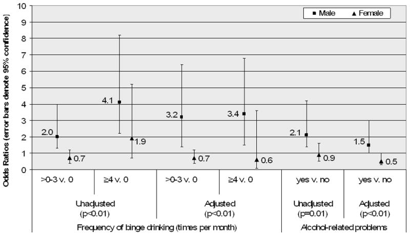
Estimated associations of neighborhood poverty (≥20% vs. <20% living in poverty) with binge drinking and alcohol-related problems across sex
Note: Here p denotes p value for the test of interaction between sex and neighborhood poverty. Frequency of binge drinking was measured as the average number of times per month the respondent binge drank in the past year. Adjusted estimates of binge drinking accounted for sex, age, race/ethnicity, income, employment, and average number of drinks per week and alcohol outlet density. Adjusted estimates of alcohol-related problems accounted for sex, age, race/ethnicity, income and employment and alcohol outlet density.
Alternative Measures of AOD
Associations of total AOD were similar to estimates of off- and on-premise AOD (data not shown). In post hoc unadjusted analysis of a binary measure of AOD, residents of high AOD areas (≥5 per 10,000 residents) compared with residents of low AOD areas (<5 per 10,000 residents) had decreased odds of binge drinking >0–3 times per month, OR = 0.7, 95% CI [0.5, 1.1], and increased odds of binge drinking ≥4 times per month, OR = 2.2, 95% CI [1.0, 4.6], compared with nonbinge drinkers (overall p value for binge drinking = .01). In adjusted analysis of the binary measure of AOD, we observed similar point estimates, residents of high AOD areas versus residents of low AOD areas were 0.8 times as likely to binge drink >0–3 times per month, 95% CI [0.5, 1.2], but were 1.5 times as likely to binge drink ≥4 times per month, 95% CI [0.6, 3.5], compared with nonbinge drinkers (overall p value for binge drinking = .36). However, the wide confidence intervals which include 1.0 (no association) in the adjusted analysis preclude us from being able to make any conclusions concerning these findings. No association was observed in unadjusted and adjusted analysis between the binary measure of AOD and alcohol-related problems (data not shown).
Discussion
We examined one mechanism linking neighborhood conditions and the occurrence of IPV in couples, hypothesizing that neighborhood poverty and greater alcohol outlet density would increase binge drinking and alcohol-related problems for drinkers in couples. We found no association between AOD and binge drinking or alcohol-related problems. However, neighborhood poverty was positively associated with both binge drinking and alcohol-related problems among male partners who drink. Neighborhood poverty was inversely associated with binge drinking and alcohol-related problems among female partners who drink, though confidence intervals were compatible with a wide range of estimates including the possibility of no association. This is the first study to examine and find that the association between neighborhood poverty and the drinking outcomes of binge drinking and alcohol-related problems may differ for men and women drinkers.
Neighborhood poverty was positively associated with binge drinking and alcohol-related problems among male drinkers and is consistent with alcohol-related violence like physical assaults that tend to be concentrated among men (U.S. Department of Justice, 2008). In couples, male binge drinking and alcohol-related problems are associated with increased rates for male perpetrated partner violence (Caetano et al., 2001). Male drinkers living in impoverished neighborhoods may binge drink more often than men in more affluent areas as a palliative escape from a stressful living environment. For example, Jones-Webb et al. (1997) reported that impoverished neighborhoods, associated with more alcohol-related problems for Black men, were characterized by low family incomes, more unemployment, and high population densities. Alternatively, it could be that a low level of collective efficacy (Sampson, Raudenbush, & Earls, 1997) inhibits residents’ ability to constrain this type of high-risk drinking. Other factors such as the types and characteristics of drinking places (e.g., cheap drinks in bars that offer minimal food vs. restaurants with more expensive drinks) may differ in wealthy and impoverished neighborhoods and may also influence binge drinking (LaVeist & Wallace, 2000). These same neighborhood characteristics may similarly increase male drinker’s risk of alcohol-related social or dependence problems.
In contrast, women living in impoverished neighborhoods may have different caretaking responsibilities and may ascribe to cultural norms that make the frequency of binge drinking lower than that found among female counterparts in wealthier areas. For example, compared with nonpoverty areas, poverty areas have a higher prevalence of larger families (1 in 25 vs. 1 in 75) and families not maintained by a married couple (35% vs. 17%; U.S. Census Bureau, 1995); both family types may be more likely to have increased caretaking responsibilities for females. Other norms and attitudes governing alcohol use as well as coping mechanisms for stress-related poverty may also differ for men and women. There is greater stigma associated with drinking for women than men (Herd, 1997). Greenfield and Room (Greenfield & Room, 1997) reported that women compared with men are less accepting of drinking and drunkenness (a characteristic related with binge drinking). It may be that women, regardless of neighborhood poverty have similar norms and attitudes about drinking. This could explain the similar associations between neighborhood impoverishment and alcohol outlets for women in poverty and nonpoverty neighborhoods. Alternatively, drinking and depression could represent different, but parallel ways of reacting to stressors for men and women, respectively (Thoits, 1995).
Our finding that AOD was not associated with binge drinking or alcohol-related problems among drinkers is somewhat surprising. Although studies of AOD and individual-level alcohol intake have been mixed (Gruenewald et al., 2002; Pollack et al., 2005; Scribner et al., 2000), many ecological studies have found positive associations between AOD and alcohol-related harms, for example, sexually transmitted diseases, motor vehicle accidents, and homicide and other violence (Cohen et al., 2006; Scribner et al., 1999; Treno et al., 2007; Zhu et al., 2004) and alcohol sales (Gruenewald, Ponicki, & Holder, 1993), which suggest that greater AOD increases individuals’ alcohol intake in that vicinity. In post hoc analysis, our binary measure of AOD showed a strong, positive association with binge drinking. However, this secondary analysis should be interpreted cautiously given it was exploratory, not hypothesized a priori and therefore may be more likely to have occurred by chance. This finding may nonetheless guide future researchers to consider whether a threshold or other measure of AOD may be a better parameterization for estimating associations between AOD and individual-level drinking measures.
Furthermore, ecological studies examining AOD and alcohol-related harms generally do not have information about the drinking status of individuals at the time the event occurred. It may be that those who experienced the harm were not drinking or may not have alcohol-related problems when it took place. Thus, there may be no association between AOD and individuals’ alcohol intake and the observed relationship with AOD may be related to other factors. For example, alternative mechanisms plausibly linking greater AOD and IPV include: (a) the loosening of normative controls against violence in disorganized neighborhoods where the number of alcohol outlets are often greater and (b) the clustering of high-risk couples in such disorganized neighborhoods (Cunradi, 2010).Furthermore, given that AOD is positively correlated with neighborhood poverty (Pollack et al., 2005), by adjusting for neighborhood poverty we may have accounted for the influence of AOD on binge drinking and alcohol-related problems. Then again, census tracts were not geographically nested within zip code boundaries, and we may have been unable to completely account for census tract–level poverty when estimating associations for AOD (and vice versa). Most studies of AOD and alcohol-related harms also do not account for individual-level sociodemographic and behavioral factors. That we were able to account for such factors could be responsible for our seemingly contradictory results. This explanation seems unlikely given that estimates for AOD were similar whether we adjusted for individual-level factors and that unadjusted estimates showed no association between AOD and binge drinking or alcohol-related problems.
Limitations of the measure of AOD, which was only available at the zip code level, may have precluded us from being able to identify associations. Our census tract–level measure of neighborhood poverty may have been a more valid and robust measure than AOD and as such, better able to detect variations in binge drinking and alcohol-related problems. Zip code–level measures of neighborhood characteristics appear less sensitive to variations in health outcomes than smaller units such as census tracts or blocks (Krieger et al., 2003a). However, in a related article (McKinney et al., 2009) based on this same survey data set we found that AOD was positively associated with IPV. We did not have the data to examine AOD using other types of measures such as number of roadway miles; others who have examined AOD using both geographic and population density measures have found that these measures yield similar findings (Scribner et al., 1999). We were also unable to analyze AOD according to specific types of alcohol outlets that may be particularly related to the examined drinking outcomes. In some studies, bars contribute disproportionately to alcohol-related social problems (Gruenewald et al., 2002; Gruenewald, Freisthler, Remer, Lascala, & Treno, 2006; Gruenewald & Remer, 2006; LaVeist & Wallace, 2000; Pollack et al., 2005). Similarly, convenience stores typically sell cold, ready-to-drink alcoholic beverages for quick consumption in large quantities (LaVeist & Wallace, 2000) and have long hours of operation. These settings may confer greater risks for binge drinking or alcohol-related problems than other types of alcohol outlets.
That is, the association between AOD and binge drinking or alcohol-related problems may exist but our inability to measure it accurately could have precluded us from observing the association. Our measure of AOD was likely subject to nondifferential misclassification since alcohol outlet data on sole proprietors and family-owned businesses were not collected by the U.S. Economic Census and we were unable to incorporate detailed alcohol-licensing laws for counties or cities into our estimates of AOD. Our measure of AOD was based on 1997 data (and poverty was based on 1990 data) and may not correspond with the environment in 1995, the time individual-level respondent data was collected and may be another source of nondifferential misclassification. In addition, where some respondents procured their alcohol may not be in the zip code in which an individual lives. These sources of misclassification may have biased our estimates.
Our findings can be generalized to drinkers who are married or cohabiting, but may not be representative of drinkers not living with a partner who may be younger and more likely to binge drink (National Institute on Alcohol Abuse and Alcoholism, 2006). Data from 1995 may not be reflective of the current situation. For example our survey collected information on binge drinking defined as ≥5 drinks for both men and women, but binge drinking was redefined in 2004 as ≥4 drinks among women and ≥5 among men (National Institute on Alcohol Abuse and Alcoholism, 2004). As fewer women would report binge drinking at ≥5 drinks than ≥4 drinks, more women would have been classified in the lower binge drinking categories (none or ≥0–3); this would bias our estimates for women drinkers toward the null. Our categorization of binge drinking was intended to capture associations of AOD and neighborhood poverty related to high-frequency binge drinking. However, our measure may not have captured certain characteristics such as the duration of this binge drinking (e.g., for how long a respondent had been binge drinking ≥4 times per month) or the peak number of drinks per binge drinking occasion. Thus, we may have not captured drinking patterns most likely associated with AOD. This notion is consistent with the “prevention paradox” which notes that drinking problems commonly occur during drinking that is generally typical (Rossow & Romelsjo, 2006; Spurling & Vinson, 2005).
In conclusion, these findings provide new information about associations of AOD and neighborhood poverty with binge drinking and alcohol-related problems in a population of married and cohabitating drinkers. Our findings suggest that male drinkers who live in high-poverty areas are at increased odds of binge drinking and having alcohol-related problems relative to male drinkers living in more affluent areas. Efforts to reduce these alcohol outcomes may have the most impact if targeted to this subpopulation. To build on this study, future research could use other analytical approaches such as structural equation modeling to detail the interrelationships between AOD, neighborhood poverty, and drinking outcomes (i.e., binge drinking and alcohol-related problems) in predicting IPV, and formally test binge drinking and alcohol-related problems as mediating variables. Our analysis used an epidemiologic approach; a geospatial approach may offer further insight. In addition, a more detailed measure of AOD at a smaller level such as census tract and being able to delineate specific types of outlets could help clarify the relationship between AOD and binge drinking and alcohol-related problems.
Acknowledgments
The authors thank Malembe Ebama and Kierste Miller for their help in preparing this article.
Funding
This work was supported by the National Institute on Alcohol Abuse and Alcoholism Grant No. R37 AA10908.
Biographies
Christy M. McKinney, PhD, MPH, is an acting assistant professor in Dental Public Health Sciences and a clinical research scholar at the Institute of Translational Health Sciences, University of Washington. She received her MPH from Tulane University and PhD from the University of Washington, both in epidemiology. Her research interests include maternal and child nutrition, oral clefts, and infant feeding in the context of global health. She is the recent recipient of an NIH Career Development Award in this area. She has also conducted research on alcohol availability, drinking, and childhood violence, and their relationships to intimate partner violence.
Karen G. Chartier, PhD, MSW, is a faculty associate at the University of Texas School of Public Health, Dallas regional campus. She completed her postdoctoral training in alcohol research at University of Connecticut School of Medicine, where she studied problem alcohol use during adolescence and early adulthood. Her research interests include ethnic group differences in drinking, alcohol problems, and alcohol treatment utilization. She earned her PhD and MSW from the University of Connecticut School of Social Work.
Raul Caetano, MD, MPH, PhD, is dean and professor of health care sciences and psychiatry, Southwestern School of Health Professions, University of Texas Southwestern Medical Center, and regional dean and professor of epidemiology, University of Texas School of Public Health. His research has focused on the epidemiology of alcohol consumption, drinking problems, and domestic violence among U.S. ethnic minorities, especially Hispanics. Another area of research is the epidemiology of alcohol dependence and the development of diagnostic criteria for alcohol dependence.
T. Robert Harris, PhD, is an associate professor of biostatistics at the University of Texas School of Public Health, Dallas Regional Campus. He has collaborated on research involving alcohol use and problems, including ethnic differences and intimate partner violence, women’s problem drinking and its risk factors including childhood sexual abuse and nontraditional employment, reliability of self-reported drinking histories, and interventions to reduce heavy drinking among young adults. He has also collaborated on research on prevalence of toxic substances in the environment.
References
- Adams Business Media. Adams liquor handbook. New York, NY: Author; 1999. On-and off-premise retail outlets-1997; pp. 308–309. [Google Scholar]
- Binder DA. On the variances of asymptotically normal estimators from complex surveys. International Statistical Review/Revue Internationale de Statistique. 1983;51:279–292. [Google Scholar]
- Caetano R, Schafer J, Cunradi CB. Alcohol-related intimate partner violence among White, Black, and Hispanic couples in the United States. Alcohol Research & Health. 2001;25:58–65. [PMC free article] [PubMed] [Google Scholar]
- Cochran WG. Sampling techniques. 3. New York, NY: John Wiley; 1977. Simple random sampling; pp. 18–44. [Google Scholar]
- Cohen DA, Ghosh-Dastidar B, Scribner R, Miu A, Scott M, Robinson P, Brown-Taylor D. Alcohol outlets, gonorrhea, and the Los Angeles civil unrest: A longitudinal analysis. Social Science and Medicine. 2006;62:3062–3071. doi: 10.1016/j.socscimed.2005.11.060. [DOI] [PMC free article] [PubMed] [Google Scholar]
- Cunradi CB. Neighborhoods, alcohol outlets, and intimate partner violence: Addressing research gaps in explanatory mechanisms. International Journal of Environmental Research and Public Health. 2010;7:799–813. doi: 10.3390/ijerph7030799. [DOI] [PMC free article] [PubMed] [Google Scholar]
- Cunradi CB, Caetano R, Clark C, Schafer J. Neighborhood poverty as a predictor of intimate partner violence among White, Black, and Hispanic couples in the United States: A multilevel analysis. Annals of Epidemiology. 2000;10:297–308. doi: 10.1016/s1047-2797(00)00052-1. [DOI] [PubMed] [Google Scholar]
- Cunradi CB, Caetano R, Clark CL, Schafer J. Alcohol-related problems and intimate partner violence among White, Black and Hispanic couples in the United States. Alcoholism: Clinical and Experimental Research. 1999;23:1492–1501. [PubMed] [Google Scholar]
- Distilled Spirits Council of the United States. Summary of state laws & regulations relating to distilled spirits. Washington, DC: Author; 1996. [Google Scholar]
- Ecob R, Macintyre S. Small area variations in health related behaviour: Do these depend on the behaviour itself, its measurement, or on personal characteristics? Health & Place. 2000;6:261–274. doi: 10.1016/s1353-8292(00)00008-3. [DOI] [PubMed] [Google Scholar]
- Ennett ST, Flewelling RL, Lindrooth RC, Norton EC. School and neighborhood characteristics associated with school rates of alcohol, cigarette, and marijuana use. Journal of Health and Social Behavior. 1997;38:55–71. [PubMed] [Google Scholar]
- Field CA, Caetano R. Ethnic differences in intimate partner violence in the U.S. general population: The role of alcohol use and socioeconomic status. Trauma Violence & Abuse. 2004;5:303–317. doi: 10.1177/1524838004269488. [DOI] [PubMed] [Google Scholar]
- Galea S, Ahern J, Tracy M, Vlahov D. Neighborhood income and income distribution and the use of cigarettes, alcohol, and marijuana. American Journal of Preventive Medicine. 2007;32:S195–S202. doi: 10.1016/j.amepre.2007.04.003. [DOI] [PMC free article] [PubMed] [Google Scholar]
- GeoLytics. CensusCD + Maps (2.0) East Brunswick, NJ: Author; 1998. [Google Scholar]
- Greenfield TK, Room R. Situational norms for drinking and drunkenness: Trends in the U.S. adult population, 1979–1990. Addiction. 1997;92:33–47. [PubMed] [Google Scholar]
- Gruenewald PJ, Freisthler B, Remer L, Lascala EA, Treno A. Ecological models of alcohol outlets and violent assaults: Crime potentials and geospatial analysis. Addiction. 2006;101:666–677. doi: 10.1111/j.1360-0443.2006.01405.x. [DOI] [PubMed] [Google Scholar]
- Gruenewald PJ, Johnson FW, Treno AJ. Outlets, drinking, and driving: A multilevel analysis of availability. Journal of Studies on Alcohol. 2002;63:460–468. doi: 10.15288/jsa.2002.63.460. [DOI] [PubMed] [Google Scholar]
- Gruenewald PJ, Ponicki WR, Holder HD. The relationship of outlet densities to alcohol consumption: A time series cross-sectional analysis. Alcoholism: Clinical and Experimental Research. 1993;17:38–47. doi: 10.1111/j.1530-0277.1993.tb00723.x. [DOI] [PubMed] [Google Scholar]
- Gruenewald PJ, Remer L. Changes in outlet densities affect violence rates. Alcoholism: Clinical and Experimental Research. 2006;30:1184–1193. doi: 10.1111/j.1530-0277.2006.00141.x. [DOI] [PubMed] [Google Scholar]
- Herd D. Racial differences in women’s drinking norms and drinking patterns: A national study. Journal of Substance Abuse. 1997;9:137–149. doi: 10.1016/s0899-3289(97)90012-2. [DOI] [PubMed] [Google Scholar]
- Hill TD, Angel RJ. Neighborhood disorder, psychological distress, and heavy drinking. Social Science & Medicine. 2005;61:965–975. doi: 10.1016/j.socscimed.2004.12.027. [DOI] [PubMed] [Google Scholar]
- Jones-Webb R, Snowden L, Herd D, Short B, Hannan P. Alcohol-related problems among Black, Hispanic, and White men: The contribution of neighborhood poverty. Journal of Studies on Alcohol. 1997;58:539–545. doi: 10.15288/jsa.1997.58.539. [DOI] [PubMed] [Google Scholar]
- Karriker-Jaffe KJ. Areas of disadvantage: A systematic review of effects of area-level socioeconomic status on substance use outcomes. Drug and Alcohol Review. 2011;30:84–95. doi: 10.1111/j.1465-3362.2010.00191.x. [DOI] [PMC free article] [PubMed] [Google Scholar]
- Karvonen S, Rimpelä AH. Urban small area variation in adolescents’ health behaviour. Social Science & Medicine. 1997;45:1089–1098. doi: 10.1016/s0277-9536(97)00036-1. [DOI] [PubMed] [Google Scholar]
- Koepsell TD, Weiss NS. Epidemiologic methods. 1. New York, NY: Oxford University Press; 2003. Confounding and its control; pp. 247–280. [Google Scholar]
- Krieger N, Chen JT, Waterman PD, Soobader MJ, Subramanian SV, Carson R. Geocoding and monitoring of US socioeconomic inequalities in mortality and cancer incidence: Does the choice of area-based measure and geographic level matter?: The public health disparities geocoding project. American Journal of Epidemiology. 2002;156:471–482. doi: 10.1093/aje/kwf068. [DOI] [PubMed] [Google Scholar]
- Krieger N, Chen JT, Waterman PD, Soobader MJ, Subramanian SV, Carson R. Choosing area based socioeconomic measures to monitor social inequalities in low birth weight and childhood lead poisoning: The public health disparities geocoding project (US) Journal of Epidemiology and Community Health. 2003a;57:186–199. doi: 10.1136/jech.57.3.186. [DOI] [PMC free article] [PubMed] [Google Scholar]
- Krieger N, Waterman PD, Chen JT, Soobader MJ, Subramanian SV. Monitoring socioeconomic inequalities in sexually transmitted infections, tuberculosis, and violence: Geocoding and choice of area-based socioeconomic measures—The public health disparities geocoding project (US) Public Health Reports. 2003b;118:240–260. doi: 10.1093/phr/118.3.240. [DOI] [PMC free article] [PubMed] [Google Scholar]
- LaVeist TA, Wallace JM., Jr Health risk and inequitable distribution of liquor stores in African American neighborhood. Social Science and Medicine. 2000;51:613–617. doi: 10.1016/s0277-9536(00)00004-6. [DOI] [PubMed] [Google Scholar]
- Leonard KE, Eiden RD. Marital and family processes in the context of alcohol use and alcohol disorders. Annual Review Clinical Psychology. 2007;3:285–310. doi: 10.1146/annurev.clinpsy.3.022806.091424. [DOI] [PMC free article] [PubMed] [Google Scholar]
- Leventhal T, Brooks-Gunn J. Moving to opportunity: An experimental study of neighborhood effects on mental health. American Journal of Public Health. 2003;93:1576–1582. doi: 10.2105/ajph.93.9.1576. [DOI] [PMC free article] [PubMed] [Google Scholar]
- Maldonado G, Greenland S. Simulation study of confounder-selection strategies. American Journal of Epidemiology. 1993;138:923–936. doi: 10.1093/oxfordjournals.aje.a116813. [DOI] [PubMed] [Google Scholar]
- McKinney CM, Caetano R, Harris TR, Ebama MS. Alcohol availability and intimate partner violence among US couples. Alcoholism: Clinical and Experimental Research. 2009;33:169–176. doi: 10.1111/j.1530-0277.2008.00825.x. [DOI] [PMC free article] [PubMed] [Google Scholar]
- Morland K, Wing S, Diez Roux A, Poole C. Neighborhood characteristics associated with the location of food stores and food service places. American Journal of Preventive Medicine. 2002;22:23–29. doi: 10.1016/s0749-3797(01)00403-2. [DOI] [PubMed] [Google Scholar]
- National Institute on Alcohol Abuse and Alcoholism. NIAAA Newsletter. 3. Bethesda, MD: Author; 2004. Winter. NIAAA council approves definition of binge drinking; p. 3. [Google Scholar]
- National Institute on Alcohol Abuse and Alcoholism. Alcohol use and alcohol use disorders in the United States: Main findings from the 2001–2002 National Epidemiologic Survey on Alcohol and Related Conditions. NIH Pub No 05–5737. Bethesda, MD: Author; 2006. Tables 1–5. Percent distribution of frequency of drinking 5 or more drinks for men or 4 or more drinks for women in a single day in the past year among current drinkers, by sex and age group, according to selected respondent characteristics, United States, 2001–2002; pp. 79–88. Retrieved from http://pubs.niaaa.nih.gov/publications/NESARC_DRM/tables/table1-5.htm. [Google Scholar]
- Peterson JB, Rothfleisch J, Zelazo PD, Pihl RO. Acute alcohol intoxication and cognitive functioning. Journal of Studies on Alcohol. 1990;51:114–122. doi: 10.15288/jsa.1990.51.114. [DOI] [PubMed] [Google Scholar]
- Pollack CE, Cubbin C, Ahn D, Winkleby M. Neighbourhood deprivation and alcohol consumption: Does the availability of alcohol play a role? International Journal of Epidemiology. 2005;34:772–780. doi: 10.1093/ije/dyi026. [DOI] [PubMed] [Google Scholar]
- Rao JNK. Small area estimation. Hoboken, NJ: John Wiley; 2003. [Google Scholar]
- Rehm J, Room R, Graham K, Monteiro M, Gmel G, Sempos CT. The relationship of average volume of alcohol consumption and patterns of drinking to burden of disease: An overview. Addiction. 2003;98:1209–1228. doi: 10.1046/j.1360-0443.2003.00467.x. [DOI] [PubMed] [Google Scholar]
- Rossow I, Romelsjo A. The extent of the prevention paradox in alcohol problems as a function of population drinking patterns. Addiction. 2006;101:84–90. doi: 10.1111/j.1360-0443.2005.01294.x. [DOI] [PubMed] [Google Scholar]
- Rothman KJ. Epidemiology: An introduction. New York, NY: Oxford University Press; 2002. Using regression models in epidemiologic analysis; pp. 181–197. [Google Scholar]
- Sampson RJ, Morenoff JD, Gannon-Rowley T. Assessing “neighborhood effects”: Social processes and new directions in research. Annual Review of Sociology. 2002;28:443–478. [Google Scholar]
- Sampson RJ, Raudenbush SW, Earls F. Neighborhoods and violent crime: A multilevel study of collective efficacy. Science. 1997;277:918–924. doi: 10.1126/science.277.5328.918. [DOI] [PubMed] [Google Scholar]
- Sayette MA, Wilson GT, Elias MJ. Alcohol and aggression: A social information processing analysis. Journal of Studies on Alcohol. 1993;54:399–407. doi: 10.15288/jsa.1993.54.399. [DOI] [PubMed] [Google Scholar]
- Scribner RA, Cohen DA, Fisher W. Evidence of a structural effect for alcohol outlet density: A multilevel analysis. Alcoholism: Clinical and Experimental Research. 2000;24:188–195. [PubMed] [Google Scholar]
- Scribner RA, Cohen D, Kaplan S, Allen SH. Alcohol availability and homicide in New Orleans: Conceptual considerations for small area analysis of the effect of alcohol outlet density. Journal of Studies on Alcohol. 1999;60:310–316. doi: 10.15288/jsa.1999.60.310. [DOI] [PubMed] [Google Scholar]
- Simons R, Johnson C, Beaman J, Conger R, Whitbeck L. Parents and peer group as mediators of the effect of community structure on adolescent problem behavior. American Journal of Community Psychology. 1996;24:145–171. doi: 10.1007/BF02511885. [DOI] [PubMed] [Google Scholar]
- Speer PW, Gorman DM, Labouvie EW, Ontkush MJ. Violent crime and alcohol availability: Relationships in an urban community. Journal of Public Health Policy. 1998;19:303–318. [PubMed] [Google Scholar]
- Spurling MC, Vinson DC. Alcohol-related injuries: Evidence for the prevention paradox. Annals of Family Medicine. 2005;3:47–52. doi: 10.1370/afm.243. [DOI] [PMC free article] [PubMed] [Google Scholar]
- Straus MA. Measuring intrafamily conflict and violence: The Conflict Tactics (CT) scales. In: Straus MA, Gelles RJ, editors. Physical violence in American families: Risk factors and adaptations to violence in 8,145 families. New Brunswick, NJ: Transaction Publishing; 1990. pp. 29–47. [Google Scholar]
- Thoits PA. Stress, coping, and social support processes: Where are we? What next? Journal of Health and Social Behavior. 1995;35:53–79. [PubMed] [Google Scholar]
- Treno AJ, Johnson FW, Remer LG, Gruenewald PJ. The impact of outlet densities on alcohol-related crashes: A spatial panel approach. Accident Analysis and Prevention. 2007;39:894–901. doi: 10.1016/j.aap.2006.12.011. [DOI] [PubMed] [Google Scholar]
- U.S. Census Bureau. Poverty in the United States: 1990: Current population reports. 175. Washington, DC: Author; 1991. Series P-60. Retrieved from http://www2.census.gov/prod2/popscan/p60-175.pdf. [Google Scholar]
- U.S. Census Bureau. Poverty areas. 1995 Retrieved from http://www.census.gov/population/socdemo/statbriefs/povarea.html.
- U.S. Census Bureau. Development of NAICS. 2001 Retrieved from http://www.census.gov/epcd/www/naicsdev.htm.
- U.S. Department of Commerce Economics and Statistics Administration. Econ 97Z report series economic census. Washington, DC: U.S. Department of Commerce, Economics and Statistics Administration; 1997. [Google Scholar]
- U.S. Department of Justice. Criminal victimization in the United States, 2006 statistical tables: National Crime Victimization Survey. Washington, DC: Author; 2008. [Google Scholar]
- Williams RL. A note on robust variance estimation for cluster-correlated data. Biometrics. 2000;56:645–646. doi: 10.1111/j.0006-341x.2000.00645.x. [DOI] [PubMed] [Google Scholar]
- Zhu L, Gorman DM, Horel S. Alcohol outlet density and violence: A geospatial analysis. Alcohol and Alcoholism. 2004;39:369–375. doi: 10.1093/alcalc/agh062. [DOI] [PubMed] [Google Scholar]