Response Properties of Local Field Potentials and Neighboring Single Neurons in Awake Primary Visual Cortex

Abstract

Recordings from local field potentials (LFPs) are becoming increasingly common in research and clinical applications, but we still have a poor understanding of how LFP stimulus selectivity originates from the combined activity of single neurons. Here, we systematically compared the stimulus selectivity of LFP and neighboring single-unit activity (SUA) recorded in area primary visual cortex (V1) of awake primates. We demonstrate that LFP and SUA have similar stimulus preferences for orientation, direction of motion, contrast, size, temporal frequency, and even spatial phase. However, the average SUA had 50 times better signal-to-noise, 20% higher contrast sensitivity, 45% higher direction selectivity, and 15% more tuning depth than the average LFP. Low LFP frequencies (<30 Hz) were most strongly correlated with the spiking frequencies of neurons with nonlinear spatial summation and poor orientation/direction selectivity that were located near cortical current sinks (negative LFPs). In contrast, LFP gamma frequencies (>30 Hz) were correlated with a more diverse group of neurons located near cortical sources (positive LFPs). In summary, our results indicate that low- and high-frequency LFP pool signals from V1 neurons with similar stimulus preferences but different response properties and cortical depths.

Introduction

The local field potential (LFP) is a measurement of the electrical activity from a local population of neurons recorded with an extracellular electrode in the brain. Although LFPs were initially thought to integrate signals within several millimeters of cortex (Mitzdorf, 1985; Juergens et al., 1999; Kreiman et al., 2006), recent studies indicate that they can be restricted to a few hundred micrometers from an electrode with a small tip (Liu and Newsome, 2006; Jin et al., 2008; Katzner et al., 2009; Xing et al., 2009; Lindén et al., 2011). Because LFP activity is easier to record and maintain than spiking activity, the recent measurements of LFP spatial specificity raise new hopes for the use of these signals in neuronal prosthetics (Andersen et al., 2004). However, to convey meaningful information about sensory cortical representations, LFP signals need to show stimulus selectivity in addition to spatial specificity. LFPs in inferotemporal cortex show robust selectivity for specific objects because neurons with similar object preferences are organized in large clusters spanning several millimeters (Kreiman et al., 2006). In middle temporal area MT, LFPs also show selectivity for speed and direction of movement because neurons with similar speed and directional tuning are organized in clusters of 0.5 and up to 2 mm (Liu and Newsome, 2006). In primary visual cortex (V1), LFPs can show certain selectivity for spatial position, orientation, and eye dominance (Berens et al., 2008a; Katzner et al., 2009; Xing et al., 2009). However, it remains unclear the extent to which the LFP stimulus selectivity conveys information about smaller clusters of neighboring single neurons (DeAngelis et al., 1999).

Just like the electroencephalogram, the LFP is divided in different frequency bands that range from 1–4 Hz (delta frequency) to 30–200 Hz (gamma frequency) when measuring stimulus-evoked activity (Fries et al., 2001; Henrie and Shapley, 2005; Bollimunta et al., 2008; Fries et al., 2008; Bosman et al., 2009; Keliris et al., 2010) and can include even higher frequencies when measuring spike-triggered single-axon LFP (Swadlow et al., 2002; Jin et al., 2008, 2011; Stoelzel et al., 2009). Previous studies have convincingly demonstrated that the stimulus selectivity of LFP is frequency dependent and that the highest LFP stimulus selectivity is found within the gamma frequency range (Frien et al., 2000; Siegel and König, 2003; Henrie and Shapley, 2005; Liu and Newsome, 2006). However, our knowledge about LFP stimulus selectivity is very limited when compared with what is known about the selectivity of single neurons in visual cortex (Hubel and Wiesel, 1962; Gilbert, 1977; DeAngelis et al., 1999; Ringach et al., 2002; Gur et al., 2005). To address this important knowledge gap, we performed a systematic comparison of response properties from LFP and neighboring single neurons in area V1 of awake macaques. We demonstrate that LFP and single-unit activity (SUA) have similar stimulus preferences, but SUA has better signal-to-noise, higher contrast sensitivity, and higher stimulus selectivity than LFP. Moreover, our results suggest that different LFP frequencies originate from different pools of neurons located at different cortical depths.

Materials and Methods

Surgery and preparation.

Monkeys (Macaca mulatta, n = 2 males) were implanted with a scleral eye coil to monitor eye movements, a head post for head fixation, and a chronic array of three to seven ultrathin electrodes protected by a recording chamber. The tip of the array was introduced through a ∼0.5 mm opening in the dura, surrounded with triple antibiotic ointment (neomycin, polymyxin B sulfates, and bacitracin zinc ointment) and placed immediately above the brain. Surgeries were performed under fully aseptic and sterile conditions. Analgesics and antibiotics were administrated before (buprenorphine, 0.01–0.02 mg/kg; cefazolin, 25 mg/kg, i.m.) and after (fentanyl patch, 3–6 μ/kg; Baytril, 5 mg/kg, i.m., for 3 days) the surgery. In preparation for the surgery, monkeys were initially sedated with an intramuscular injection of chlorpromazine (1 mg/kg, i.m.), ketamine (5–15 mg/kg, i.m.), and atropine (0.05 mg/kg, i.m.). General anesthesia was induced with intravenous thiopental (5–15 mg/kg, i.v.) and maintained with a mixture of isoflurane (0.5–2%) and oxygen (30%). Temperature, electrocardiogram, blood pressure, and expired CO₂ were continuously monitored to ensure adequate anesthesia and ventilation. During the entire surgical procedure, the eyes were kept closed and lubricated with ophthalmic ointment to protect the corneas. All procedures were performed in accordance with the guidelines of the U.S. Department of Agriculture and approved by the Institutional Animal Care and Use Committee at the State University of New York, State College of Optometry.

Visual stimuli.

Visual stimuli were generated with a computer running Visionworks (Vision Research Graphics) and presented on a GDM-F520 monitor (Sony Electronics; refresh rate, 160 Hz; mean luminance, 61 cd/m²; resolution, 640 × 480 pixels). The spatiotemporal receptive fields were mapped with Hartley stimuli (Ringach et al., 1997) and sparse noise (Jones and Palmer, 1987) to accurately measure the eccentricity and center the grating stimulus that was used to test other response properties. The Hartley stimulus consisted of 576 gratings with different orientations, phases, and spatial frequencies randomly presented at 80 Hz. The sparse noise consisted of bright and dark squares (0.2–0.4°/side) randomly presented at 16 × 16 different positions at 25 Hz. Most response properties quantified in this study were measured with drifting gratings presented for 2–3 s at 2–4 Hz (usually three to four presentations per stimulus parameter). Static gratings presented at 1 Hz were used for the measurements of spatial phase. Orientation/direction tuning was measured with 16 different directions (eight orientations), contrast sensitivity with eight different contrasts (0–76%), size tuning with eight different sizes (0.6–8°), phase selectivity with 10 different phases (0–0.9 cycles), and temporal frequency tuning with nine different temporal frequencies (0.5–30 Hz), with both drifting and flickering gratings.

The monkeys were trained to touch a bar and fixate a small cross (0.1°/side) presented at a distance of 57 cm. They maintained the eye position within ±0.5–1° for 2–3 s and released the bar when the cross changed color to receive a drop of juice as reward. During the 2–3 s of fixation, stimuli were presented at the receptive field location of the recorded single neuron to study the response properties of the single neuron and LFP.

Data collection and analysis.

V1 cortical activity was recorded with a chronically implanted array of three to seven ultrathin electrodes (1 μm tip, 15 μm shaft, 100–200 μm² exposed metal area), with each electrode separated from its neighbor by ∼150 μm. The electrodes were made of platinum–alloy core (90% platinum and 10% tungsten) covered with quartz (40 μm in diameter) and had impedances of 1–3 MΩ. The electrodes were independently moved with individual microdrives (Swadlow et al., 2005; Chen et al., 2008), and the electrical signals from each electrode were collected amplified, digitized, and filtered either between 250 Hz and 8 kHz (spikes) or between 0.5 Hz and 2.2 kHz (LFPs) with a two-pole low-cut and four-pole high-cut filters. Spikes and LFPs were sampled at 40 and 5 kHz, respectively (Plexon). Eye movements were sampled at 5 kHz. Spikes from single neurons were convolved with a Gaussian function (σ = 2 ms) to generate a continuous spike density signal. The LFP raw signal was low-pass filtered (<500 Hz) with a fourth-order Butterworth filter. A fast Fourier transform (FFT function in MATLAB; version R2007b) was used to convert spike density and LFP signals into different frequency bands: delta (1–4 Hz), theta (4–8 Hz), alpha (8–12 Hz), beta (12–30 Hz), low-gamma (30–90 Hz), and high-gamma (90–200 Hz) frequencies.

To make quantitative comparisons of the response properties between LFP and neighboring single neurons, we used different fitting functions. Orientation tuning was fitted with a von Mises function described by Equation 1 (Swindale et al., 2003):

where Rϕ is the response amplitude to each stimulus orientation (ϕ), A₁ and A₂ are the response amplitudes for the two opposite directions of movement (ϕ₁ and ϕ₂), and k₁ and k₂ are the inverses of the tuning widths.

Contrast sensitivity and size tuning were fitted with hyperbolic ratio functions (Naka and Rushton, 1966; Peirce, 2007), as described by Equation 2:

where Rc is the response to each contrast/size, B is the baseline activity, R_max is the maximum response (with baseline subtracted), C is each stimulus contrast/size, C₅₀ is the contrast/size that generate half-maximum response, and n and s are the exponents that control the shape of function.

Phase and temporal frequency tuning were fitted with Gaussian functions, as described by Equation 3:

where Rx is the response to each x parameter (e.g., each phase), A is the maximum amplitude of the function, μ is the mean (the peak phase/temporal frequency of the Gaussian), σ is the SD (the width of the Gaussian), and B is the baseline activity.

Comparisons were restricted to tuning functions with reasonable goodness of fit (R ≥ 0.6). This selection included 113 recordings for orientation, 54 recordings for contrast response functions, 31 recordings for size tuning, 71 recordings for spatial phase tuning, and 23 recordings for temporal frequency tuning (18 recordings measured with flickering gratings and five with drifting gratings). We excluded from our analysis LFP recordings that showed poor responses to visual stimuli. We did not use any type of filtering to remove power line 60 Hz noise because it had small amplitude in most recordings. All tuning functions were normalized by dividing the mean frequency power of the response by the mean frequency power of the baseline activity preceding the stimulus onset (−200 to 0 ms). Therefore, the units of the tuning functions are given as multiples of the signal/noise ratio of the recordings, as described by Equation 4:

where SNR is the signal/noise ratio, r_Si is the mean frequency power of the response to stimulus Si, r_b is the mean frequency power of the baseline activity, and n is the number of stimulus trials (usually three to four). For neurons that had no spontaneous firing rate, we assigned an arbitrary baseline rate of 0.01 spikes/s. To compare the mean signal/noise ratio of LFP and SUA, we either averaged all measurements of signal-to-noise (signal/noise ratio) or excluded the measurements from neurons with zero spontaneous activity [signal/noise (no zero baselines)].

Direction selectivity (DS) was measured as described in Equation 5:

where A₁ and A₂ are the response amplitudes to the two directions of movement at the preferred orientation. The DS is 0 if the neuronal responses to both directions of movement are the same (A₁ = A₂) and 1 if the neuronal responses are restricted to only one direction (e.g., A₁ = 0).

The same equations were used to measure the tuning functions for single neurons and LFPs. The stimulus tuning for the entire cell population was calculated by adding the tuning functions measured at each recording site, after normalizing each function by its maximum response. For orientation and phase tuning, this addition was performed after aligning all the tuning functions with the preferred orientation (or phase) at each recording site (the central bin was removed and replaced by the interpolation of the bins on the sides of the central bin). Tuning depth was measured as the difference between the maximum and minimum of the tuning curve divided by the maximum.

We estimated the cortical depth of the recordings by measuring the polarity of the LFP, which becomes increasingly negative as the electrode approaches the middle layers of the cortex and reverses polarity when it reaches the deep layers. The polarity of the LFP was calculated by measuring the LFP integral between 0 and 60 ms after the stimulus onset. We also measured the spike-field coherence to estimate the correlation between the frequency spectrum of spikes and LFPs. The spike-field coherence was computed using an open-source Chronux library for MATLAB (Bokil et al., 2010), a sliding window of 200 ms, and nine tapers. We measured the average coherence at low frequencies (1–30 Hz), gamma frequencies (30–200 Hz), and the low/gamma ratio. For each single neuron, we also measured the spike amplitude (from peak to trough) and spike width (from spike onset to maximum absolute value of trough).

Results

We used chronically implanted arrays of ultrathin electrodes to simultaneously record from LFPs and neighboring SUA with the same electrode tip from area V1 of awake macaques. We compared the visual responses of well-isolated single neurons (Fig. 1A) with the visual responses of LFPs measured at different frequency bands (Fig. 1B). The recordings were highly stable, and single units could be maintained regularly for several hours and occasionally for several days or weeks (Fig. 1C). We studied the tuning of SUA/LFP pairs for different stimulus properties, including orientation, direction of movement, luminance contrast, size, spatial phase, and temporal frequency. To perform accurate comparisons between SUA and LFP, we transformed the spike trains into a continuous spike density histogram and measured SUA and LFP histograms at the same frequency bands: delta (1–4 Hz), theta (4–8 Hz), alpha (8–12 Hz), beta (12–30 Hz), low gamma (30–90 Hz), and high gamma (90–200 Hz). Although some single neurons were tuned across all spiking frequency bands (Fig. 2A), most neurons were better tuned at some frequencies than others (Fig. 2B), and, in the entire SUA population, the spiking frequency spectrum was better tuned at low-frequency (<8 Hz) and high-frequency (>30 Hz) bands than intermediate ones (Fig. 2C). Because most LFPs showed strong responses to the stimulus onset, we measured stimulus tuning separately for the first 200 ms of the response (stimulus transient) and the remaining response (sustained stimulation).

Figure 1.

Experimental approach to record SUA and LFPs from the same electrode tip. A, Example of a single-unit recording shown as superimposed waveforms of both single-unit (blue) and multiunit (gray), average of the waveforms (continuous lines), SD (dashed lines), and waveform sorting. B, Spike rasters (top black trace) were convolved with a Gaussian function (σ = 2 ms) to generate a continuous spike density signal (bottom black trace). LFPs were low-pass filtered at <500 Hz (top blue trace), and a fast Fourier transform was applied to calculate the power at different frequency bands (bottom blue traces). C, Recording stability for both SUA and LFP was excellent. This example shows a case in which we recorded a spike waveform for several consecutive days. Over these days, the spike waveform remained relatively unchanged (although increased in amplitude on the second week). The response properties were also very similar across days (shown here are the spatiotemporal receptive field and orientation/direction tuning). Trans, Transient.

Figure 2.

SUA stimulus tuning at different frequency bands. A, Example of SUA with robust orientation tuning that can be demonstrated across all frequency bands. Notice that the tuning is stronger at low (delta and theta) and high [low-gamma (LGF) and high-gamma (HGF) frequencies] than at intermediate frequency bands (alpha, beta). Left, Spike rasters from SUA evoked by a grating drifting at 16 different directions (3 trials per direction). Right, Orientation tuning calculated at different frequency bands. B, Example of SUA with robust orientation tuning limited to low (delta, theta) and high (LGF, HGF) frequency bands. C, Histogram showing the number of SUA, MUA, and LFP that had significant orientation tuning (R ≥ 0.6) at a given frequency band. Notice that there were more recordings with significant tuning at low (delta, theta) and high (LFG, HGF) than at intermediate (alpha, beta) frequency bands. Trans, Transient.

Orientation and direction tuning

Consistent with previous studies, the most robust LFP orientation tuning was demonstrated at the highest LFP frequencies during sustained stimulation with drifting gratings (Frien et al., 2000; Siegel and König, 2003; Henrie and Shapley, 2005; Liu and Newsome, 2006). Figure 3 illustrates a recording from a V1 single neuron with sharp orientation tuning (Fig. 3A) measured at the gamma frequency band of the spike density histogram, both at the stimulus transient and during sustained stimulation (drifting grating; Fig. 3B). In contrast to the single neuron, the LFP responded robustly to all stimulus transients (Fig. 3C), but it also showed pronounced orientation tuning at the gamma frequency band when the grating was drifting. The orientation preferences for the high-gamma LFP and SUA were matched, but the tuning bandwidth was broader for the high-gamma LFP (Fig. 3D).

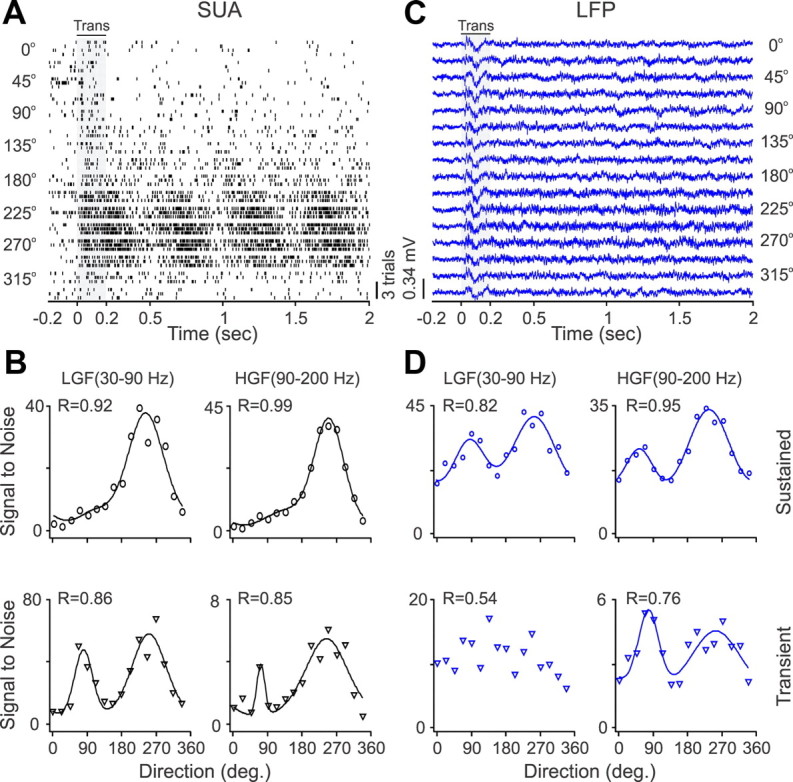
Figure 3.

SUA/LFP orientation tuning for an example recording site. A, Spike rasters from SUA evoked by a grating drifting at 16 different directions (3 trials per direction). The grating starts drifting at 0 s, and the baseline activity is measured from −0.2 to 0 s, the transient response (Trans) from 0 to 0.2 s (shaded area), and the response to sustained stimulation from 0.2 to 2 s. B, The neuron had sharp orientation tuning illustrated for two different frequency bands, low-gamma frequency (LGF) and high-gamma frequency (HGF) at the response transient and during sustained stimulation (drifting grating). R values illustrate the goodness of fit. C, LFPs recorded from the same electrode tip than SUA responding to different grating directions marked on the right side of the figure. LGF, Low-gamma frequency; HGF, high-gamma frequency. D, LFP orientation tuning shown for the same two frequency bands than SUA in C. LFP and SUA orientation preferences were similar but the tuning was broader and shallower in LFP than SUA.

Gamma LFP was not only tuned for orientation but also for the direction of movement. Figure 4 shows another example of a single cell with broad orientation tuning and strong direction selectivity (Fig. 4A,B). As in the previous example, the LFP responded to all stimulus transients (Fig. 4C), but it showed significant orientation/direction selectivity at the gamma frequency band during sustained stimulation (Fig. 4D). The gamma LFP and SUA had similar orientation and direction preferences, but the direction selectivity was weaker for the LFP than SUA (Fig. 4D). We measured the orientation/direction tuning of multiple SUA/LFP paired recordings and fitted the tuning curves with a von Mises function (Swindale et al., 2003) separately for each frequency band. Reasonable good fits (R ≥ 0.6) could be demonstrated for both LFP and SUA across all frequency bands, but the number of fits that passed our criterion and the average goodness of fit were larger for SUA than LFPs (Fig. 5A, Table 1). To compare the average orientation tuning of SUA and LFP, we aligned all LFP orientation tuning curves with R ≥ 0.6, normalized them by their maximum value, and then averaged them separately for each frequency band. This analysis revealed greater tuning depth in high-gamma SUA than high-gamma LFP recordings (Fig. 5B, Table 2). The orientation preferences of LFP and SUA were significantly correlated at the low-gamma (r = 0.58, p = 0.002) and high-gamma (r = 0.69, p = 0.00001) frequency during sustained stimulation and at the high-gamma frequency (r = 0.79, p = 0.001) during the stimulus transient (Table 3). The direction selectivity of LFP and SUA were significantly correlated at the high-gamma frequency band during sustained stimulation (r = 0.47, p = 0.0008) and at the delta frequency band during the stimulus transient (r = 0.44, p = 0.016). These results demonstrate that, although all frequency bands of LFP can show certain orientation/direction tuning, LFP has less tuning depth than SUA, and the best correlation between the stimulus preferences of LFP and SUA is at the gamma frequency band for orientation and at the gamma frequency and delta frequency for direction selectivity [note that the delta frequency contains the frequency of the drifting grating (2–4 Hz)].

Figure 4.

SUA/LFP direction tuning for an example recording site. A, Spike rasters from SUA stimulated with gratings drifting at 16 different directions (3 trials per direction). B, The neuron had strong direction selectivity, which is illustrated for two different frequency bands at the response transient (Trans) and during sustained stimulation (drifting grating). C, LFP responses to different directions of movement. D, LFP had weaker direction selectivity than SUA. LGF, Low-gamma frequency; HGF, high-gamma frequency.

Figure 5.

Population analysis for SUA/LFP orientation and direction selectivity. A, Distributions of goodness of fit (R) for SUA (black) and LFP (blue) measured at different frequency bands during sustained stimulation (Sust., top) and stimulus transient (Trans., bottom). The distribution is shown only for recording sites that passed our criterion (R ≥ 0.6). B, Average orientation tuning for SUA (black) and LFP (blue) during sustained and transient stimulation, measured at different frequency bands. The orientation tuning curves were aligned at 45°, normalized by the maximum response and then averaged together. The bin at 45 ° was then subtracted and interpolated using the two adjacent bins (22.5 and 67.5). Tuning curves with a mean closer to 1 (e.g., LFP sustained at high-gamma frequency) have lower signal-to-noise than those with a mean closer to 0 (e.g., SUA sustained at delta frequency). LGF, Low-gamma frequency; HGF, high-gamma frequency.

Table 1.

Average goodness of fit of SUA and LFP recordings

	Delta (1–4 Hz)	Theta (4–8 Hz)	Alpha (8–12 Hz)	Beta (12–30 Hz)	LGF (30–90 Hz)	HGF (90–200 Hz)
SUA versus LFP (sustained)
Orientation/direction	R = 0.88/0.76	R = 0.85/0.73	R = 0.8/0.75	R = 0.8/0.71	R = 0.84/0.73	R = 0.83/0.77
	n = 95/50	n = 76/33	n = 57/36	n = 69/23	n = 71/31	n = 84/59
	p < 0.00001	p = 0.002	p = 0.21	p = 0.26	p < 0.00001	p < 0.00001
Contrast	R = 0.93/0.83	R = 0.88/0.81	R = 0.84/0.81	R = 0.88/0.77	R = 0.94/0.93	R = 0.93/0.95
	n = 51/42	n = 50/34	n = 42/25	n = 50/25	n = 53/50	n = 53/50
	p < 0.00001	p = 0.01	p = 0.35	p = 0.001	p = 0.26	p = 0.26
Size	R = 0.84/0.74	R = 0.78/0.82	R = 0.78/0.71	R = 0.76/0.81	R = 0.85/0.88	R = 0.84/0.89
	n = 21/18	n = 22/19	n = 17/11	n = 25/23	n = 24/28	n = 27/24
	p = 0.12	p = 0.36	p = 0.01	p = 0.65	p = 0.01	p = 0.026
Phase	R = 0.89/0.76	R = 0.87/0.77	R = 0.85/0.79	R = 0.84/0.75	R = 0.84/0.75	R = 0.84/0.77
	n = 55/23	n = 50/28	n = 45/26	n = 49/14	n = 45/26	n = 51/28
	p = 0.00001	p = 0.002	p = 0.03	p = 0.12	p = 0.02	p = 0.01
Temporal frequency	R = 0.89/0.88	R = 0.87/0.91	R = 0.91/0.92	R = 0.91/0.89	R = 0.91/0.86	R = 0.89/0.85
	n = 21/15	n = 19/15	n = 17/19	n = 22/16	n = 20/18	n = 21/15
	p = 0.72	p = 0.71	p = 0.83	p = 0.45	p = 0.27	p = 0.44
SUA versus LFP (transient)
Orientation/direction	R = 0.88/0.73	R = 0.84/0.73	R = 0.82/0.71	R = 0.77/0.7	R = 0.8/0.7	R = 0.79/0.72
	n = 92/35	n = 82/29	n = 71/34	n = 54/23	n = 58/25	n = 64/25
	p < 0.00001	p = 0.00001	p = 0.00001	p = 0.008	p = 0.006	p = 0.14
Contrast	R = 0.92/0.89,	R = 0.9/0.86	R = 0.86/0.88	R = 0.87/0.87	R = 0.86/0.89	R = 0.87/0.89
	n = 49/41	n = 51/45	n = 42/43	n = 39/45	n = 45/49	n = 49/45
	p = 0.22	p = 0.13	p = 0.38	p = 0.86	p = 0.26	p = 0.69
Size	R = 0.83/0.81	R = 0.77/0.79	R = 0.78/0.8	R = 0.78/0.76	R = 0.74/0.8	R = 0.76/0.81
	n = 19/14	n = 21/16	n = 11/16	n = 11/19	n = 23/25	n = 18/21
	p = 0.25	p = 0.44	p = 0.46	p = 0.37	p = 0.14	p = 0.23
Phase	R = 0.89/0.76	R = 0.86/0.81	R = 0.82/0.78	R = 0.84/0.79	R = 0.82/0.78	R = 0.83/0.79
	n = 53/19	n = 44/24	n = 46/23	n = 37/27	n = 37/14	n = 43/42
	p = 0.06	p = 0.009	p = 0.44	p = 0.15	p = 0.11	p = 0.25
Temporal frequency	R = 0.87/0.84	R = 0.88/0.81	R = 0.83/0.86	R = 0.89/0.81	R = 0.88/0.79	R = 0.87/0.86
	n = 18/9	n = 18/10	n = 15/10	n = 18/14	n = 15/16	n = 15/14
	p = 0.88	p = 0.07	p = 0.8	p = 0.1	p = 0.09	p = 0.82

Each row provides the average goodness of fit (R) for SUA/LFP, followed by the number of recording sites that had R ≥ 0.6 for SUA/LFP, followed by the p value obtained by comparing the LFP and SUA means (t test). Recordings with R < 0.6 were not included in the mean comparisons. Significant differences are highlighted in bold. LGF, Low-gamma frequency; HGF, high-gamma frequency.

Table 2.

Response selectivity of SUA and LFP recordings

	Delta (1–4 Hz)	Theta (4–8 Hz)	Alpha (8–12 Hz)	Beta (12–30 Hz)	LGF (30–90 Hz)	HGF (90–200 Hz)
SUA versus LFP (sustained)
Direction selectivity	0.53/0.48	0.54/0.4	0.48/0.46	0.3/0.28	0.39/0.2	0.37/0.16
	p = 0.35	p = 0.07	p = 0.87	p = 0.72	p = 0.003	p < 0.00001
Orientation tuning depth	0.89/0.85	0.9/0.83	0.91/0.81	0.77/0.64	0.82/0.57	0.79/0.48
	p = 0.04	p = 0.004	p = 0.001	p = 0.005	p < 0.00001	p < 0.00001
Contrast tuning depth	0.97/0.87	0.94/0.78	0.93/0.78	0.82/0.56	0.82/0.66	0.84/0.62
	p < 0.00001	p < 0.00001	p < 0.00001	p < 0.00001	p < 0.00001	p < 0.00001
Size tuning depth	0.92/0.86	0.93/0.85	0.90/0.77	0.79/0.6	0.79/0.68	0.82/0.66
	p = 0.33	p = 0.002	p = 0.007	p < 0.00001	p = 0.01	p < 0.00001
Phase tuning depth	0.95/0.89	0.97/0.91	0.96/0.92	0.92/0.73	0.87/0.65	0.86/0.62
	p = 0.008	p = 0.007	p = 0.01	p = 0.02	p < 0.00001	p < 0.00001
Temporal tuning depth	0.91/0.92	0.87/0.9	0.9/0.93	0.76/0.82	0.73/0.78	0.65/0.59
	p = 0.77	p = 0.45	p = 0.51	p = 0.33	p = 0.39	p = 0.35
Contrast (C50)	35.95/28.08	30.03/31.19	28.17/38.25	10.84/25.55	10.72/18.64	11.41/10.55
	p = 0.059	p = 0.85	p = 0.07	p = 0.005	p = 0.00009	p = 0.6
Size (S50)	2.28/2.78	2.06/3.26	1.73/0.9	1.37/1.44	1.75/1.92	1.67/1.28
	p = 0.23	p = 0.07	p = 0.1	p = 0.65	p = 0.28	p = 0.03
Contrast (exponent)	3.09/11.7	5.9/13.5	9.67/11.68	4.72/11.34	4.04/4.39	3.46/5.21
	p < 0.00001	p = 0.003	p = 0.51	p = 0.02	p = 0.73	p = 0.036
Size (exponent)	12.52/18.03	15/13.41	3.4/2.96	8.21/12	8.4/7.65	8.45/4.66
	p = 0.43	p = 0.72	p = 0.94	p = 0.27	p = 0.77	p = 0.029
Signal/noise	616660/45	140210/59	7309/29	4655/16	2682/48	1809/41
	p = 0.008	p = 0.008	p = 0.008	p = 0.055	p = 0.095	p = 0.008
Signal/noise (no zero baseline)	3754/45	2380/59	698/29	398/16	370/48	357/41
	p = 0.008	p = 0.008	p = 0.016	p = 0.055	p = 0.095	p = 0.008
SUA versus LFP (transient)
Direction selectivity	0.74/0.47	0.55/0.43	0.59/0.36	0.49/0.26	0.37/0.3	0.56/0.27
	p = 0.0001	p = 0.23	p = 0.003	p = 0.067	p = 0.37	p = 0.002
Orientation tuning depth	0.94/0.85	0.92/0.82	0.97/0.82	0.92/0.73	0.88/0.7	0.91/0.68
	p < 0.00001	p = 0.016	p = <0.00001	p < 0.00001	p < 0.00001	p < 0.00001
Contrast tuning depth	0.97/0.97	0.97/0.96	0.97/0.96	0.95/0.9	0.9/0.82	0.92/0.77
	p = 0.95	p = 0.18	p = 0.36	p = 0.004	p < 0.00001	p < 0.00001
Size tuning depth	0.95/0.90	0.97/0.88	0.97/0.88	0.94/0.91	0.87/0.85	0.87/0.77
	p = 0.13	p = 0.009	p = 0.27	p = 0.38	p = 0.45	p = 0.06
Phase tuning depth	0.89/0.83	0.91/0.77	0.95/0.79	0.91/0.69	0.92/0.75	0.86/0.65
	p = 0.2	p = 0.003	p < 0.00001	p = 0.006	p = 0.04	p < 0.00001
Temporal tuning depth	0.85/0.84	0.88/0.8	0.97/0.87	0.91/0.77	0.84/0.67	0.79/0.67
	p = 0.92	p = 0.19	p = 0.01	p = 0.018	p = 0.003	p = 0.12
Contrast (C50)	17.28/19.39	21.07/24.82	23.49/23.08	20.43/24.69	15.13/23.85	13.77/16.30
	p = 0.46	p = 0.21	p = 0.007	p = 0.22	p = 0.0008	p = 0.17
Size (S50)	1.87/1.25	1.93/0.79	3.35/2.2	2.08/0.88	1.79/2.16	1.85/1.4
	p = 0.2	p = 0.009	p = 0.5	p = 0.03	p = 0.31	p = 0.13
Contrast (exponent)	5.14/10.42	7.15/11.3	10.08/9.4	8.76/8.44	7.94/7.6	8.04/5.70
	p = 0.001	p = 0.04	p = 0.77	p = 0.87	p = 0.8	p = 0.064
Size (exponent)	10.45/6.9	13.66/3.56	3.02/6.94	12.21/4.14	8.62/7.52	11.44/6.59
	p = 0.51	p = 0.003	p = 0.47	p = 0.14	p = 0.8	p = 0.14
Signal/noise	307320/462	62723/986	2401/848.45	3238/182.63	1153/26.44	359/9.08
	p = 0.008	p = 0.016	p = 0.09	p = 0.008	p = 0.008	p = 0.016
Signal/noise (no zero baseline)	118290/462	15857/986	2401/848.45	1561/182.63	554/25.88	73/9.08
	p = 0.008	p = 0.016	p = 0.09	p = 0.055	p = 0.09	p = 0.016

Each row provides the mean response selectivity of SUA/LFP for each response property listed on the left column, followed by the p value obtained by comparing the SUA/LFP means (t test). Significant differences are highlighted in bold. LGF, Low-gamma frequency; HGF, high-gamma frequency.

Table 3.

Correlations between SUA and LFP response properties

	Delta (1–4 Hz)	Theta (4–8 Hz)	Alpha (8–12 Hz)	Beta (12–30 Hz)	LGF (30–90 Hz)	HGF (90–200 Hz)
SUA versus LFP (sustained)
Orientation preference	r = 0.13	r = −0.37	r = −0.05	r = 0.3	r = 0.58	r = 0.69
	p = 0.4	p = 0.09	p = 0.85	p = 0.28	p = 0.002	p = 0.00001
	n = 44	n = 21	n = 16	n = 15	n = 25	n = 48
Direction selectivity	r = 0.07	r = 0.1	r = −0.04	r = 0.39	r = 0.21	r = 0.47
	p = 0.66	p = 0.67	p = 0.88	p = 0.15	p = 0.31	p = 0.0008
	n = 44	n = 21	n = 16	n = 15	n = 25	n = 48
Contrast (C50)	r = 0.22	r = −0.14	r = 0.38	r = 0.13	r = 0.24	r = 0.4
	p = 0.16	p = 0.46	p = 0.08	p = 0.57	p = 0.1	p = 0.005
	n = 41	n = 30	n = 22	n = 23	n = 49	n = 49
Size (S50)	r = 0.3	r = −0.18	r = 0.41	r = 0.69	r = 0.38	r = 0.49
	p = 0.33	p = 0.52	p = 0.35	p = 0.001	p = 0.07	p = 0.017
	n = 12	n = 15	n = 7	n = 19	n = 23	n = 23
Phase preference	r = −0.21	r = −0.31	r = −0.33	r = 0.63	r = 0.37	r = 0.57
	p = 0.39	p = 0.178	p = 0.17	p = 0.09	p = 0.126	p = 0.008
	n = 18	n = 20	n = 16	n = 8	n = 18	n = 20
Temporal frequency preference	r = −0.08	r = −0.15	r = −0.047	r = −0.15	r = 0.049	r = 0.033
	p = 0.78	p = 0.59	p = 0.87	p = 0.57	p = 0.85	p = 0.91
	n = 14	n = 14	n = 14	n = 15	n = 16	n = 13
SUA versus LFP (transient)
Orientation preference	r = 0.29	r = 0.16	r = 0.22	r = 0.1	r = 0.54	r = 0.79
	p = 0.13	p = 0.49	p = 0.37	p = 0.77	p = 0.057	p = 0.001
	n = 29	n = 21	n = 18	n = 11	n = 13	n = 12
Direction selectivity	r = 0.44	r = −0.03	r = 0.23	r = 0.2	r = 0.35	r = 0.46
	p = 0.016	p = 0.91	p = 0.35	p = 0.56	p = 0.24	p = 0.11
	n = 29	n = 21	n = 18	n = 11	n = 13	n = 13
Contrast (C50)	r = 0.12	r = 0.31	r = 0.43	r = 0.14	r = −0.21	r = 0.32
	p = 0.47	p = 0.04	p = 0.013	p = 0.43	p = 0.18	p = 0.039
	n = 38	n = 42	n = 32	n = 34	n = 41	n = 41
Size (S50)	r = 0.56	r = 0.44	r = 0.7	r = 0.88	r = −0.01	r = 0.42
	p = 0.09	p = 0.15	p = 0.5	p = 0.02	p = 0.97	p = 0.15
	n = 10	n = 12	n = 3	n = 6	n = 20	n = 13
Phase preference	r = −0.028	r = 0.31	r = 0.039	r = 0.018	r = −0.66	r = 0.42
	p = 0.92	p = 0.19	p = 0.89	p = 0.96	p = 0.22	p = 0.033
	n = 15	n = 18	n = 14	n = 10	n = 5	n = 26
Temporal frequency preference	r = −0.22	r = 0.78	r = −0.3	r = −0.17	r = 0.4	r = 0.45
	p = 0.62	p = 0.022	p = 0.49	p = 0.65	p = 0.19	p = 0.16
	n = 7	n = 8	n = 7	n = 9	n = 12	n = 11

Each row provides the correlation value for each SUA/LFP response property listed on the left column, followed by the p value and number of recordings. Both the SUA and LFP goodness of fit had to be ≥0.6 for each frequency band to be included in the correlation analysis. Significant differences are highlighted in bold. LGF, Low-gamma frequency; HGF, high-gamma frequency.

Contrast and size tuning

LFP visual responses are known to increase with luminance contrast (Henrie and Shapley, 2005), but the contrast response functions of LFP and SUA have not been quantitatively compared. Here, we took advantage of the robust LFP modulation to stimulus contrast to perform this comparison. Figure 6 illustrates a single neuron (Fig. 6A,B) and LFP (Fig. 6C,D) whose visual responses increased steeply with luminance contrasts larger than 4%. As illustrated in this example, the contrast response functions of LFP and SUA were not identical. For example, at the low-gamma frequency band, the contrast response function was more linear and had higher C₅₀ (contrast generating half-maximum response) in the LFP (Fig. 6D) than the SUA recordings (Fig. 6B). Both SUA and LFP contrast response functions were well fit with a hyperbolic function (Fig. 7A, Table 1), but the function had greater response range (greater tuning depth) and lower C₅₀ in SUA than LFP recordings (Fig. 7B, Table 2). The C₅₀ of LFP and SUA were correlated at different frequency bands, including the high-gamma band during sustained (r = 0.4, p = 0.005) and transient stimulation (r = 0.32, p = 0.039) and the theta band (r = 0.31, p = 0.04) and alpha band (r = 0.43, p = 0.013) during transient stimulation (Table 3).

Figure 6.

SUA/LFP contrast response functions for an example recording site. A, Spike rasters from SUA stimulated with drifting gratings at eight different contrasts (4 trials per contrast). B, The neuron had a steep and nonlinear contrast response function, which is illustrated for the spike densities measured at two different frequency bands. C, LFP responses to gratings with different contrasts. D, LFP contrast response functions. LGF, Low-gamma frequency; HGF, high-gamma frequency; Trans., transient.

Figure 7.

Population analysis for SUA/LFP contrast response functions. A, Distributions of goodness of fit for SUA and LFP contrast response functions. B, Average contrast response functions after normalizing each function by the maximum value and then averaging SUA and LFP separately for each frequency band. LGF, Low-gamma frequency; HGF, high-gamma frequency; Trans., transient; Sust., sustained.

Although the results described above demonstrate that SUA has better stimulus selectivity and higher contrast sensitivity than LFP, the stimulus size that generated half-maximum response (S₅₀) was frequently smaller for LFP than SUA. Figure 8 illustrates an example of a recording from a V1 neuron and LFP that had different size tuning. Although the response of the V1 neuron increased steadily with stimulus size (Fig. 8A,B), the LFP saturated at 1.2–2.3 ° and was more suppressed by stimuli of larger size (Fig. 8C,D). At most frequency bands, the LFP and SUA size tuning had similar average goodness of fit (Fig. 9A). However, at the gamma band during sustained stimulation, the average goodness of fit was actually higher for LFP than SUA (low-gamma SUA/LFP, 0.85/0.88, p = 0.01; high-gamma SUA/LFP, 0.84/0.89, p = 0.026; Table 1). Interestingly, although SUA had greater tuning depth than LFP (Fig. 9B, Table 2), the S₅₀ was still lower for LFP, a finding that could be demonstrated in individual recordings (Fig. 8A,C) and in the average of all recordings at different frequency bands (e.g., high-gamma band during sustained stimulation, theta and beta band during the stimulus transient; Table 2). Moreover, the S₅₀ of LFP and SUA were correlated at different frequency bands (high-gamma and beta bands during sustained stimulation and beta band during the stimulus transient; Table 3). We cannot completely discard the possibility that some of the differences in size tuning between LFP and SUA could be caused by small misalignments between the stimulus and the receptive field center; these misalignments would affect more the SUA than LFP because the LFP receptive field is larger. However, clear differences in size tuning could still be demonstrated in cells in which we mapped the receptive fields with reverse correlation multiple times to identify the smallest stimulus size that generated a reliable receptive field map (e.g., recording from Fig. 8).

Figure 8.

SUA/LFP size tuning for an example recording site. A, Spike rasters from a single neuron that responded to grating patches >1.2°. B, SUA size tuning illustrated for two different frequency bands. C, LFP responses to gratings of different sizes. Notice that the LFP responded better to smaller gratings than the SUA. D, LFP size tuning. LGF, Low-gamma frequency; HGF, high-gamma frequency; Trans., transient.

Figure 9.

Population analysis for SUA/LFP size tuning. A, Distributions of goodness of fit for SUA and LFP size tuning. B, Average size tuning functions after normalizing each function by the maximum value and then averaging SUA and LFP separately for each frequency band. LGF, Low-gamma frequency; HGF, high-gamma frequency; Trans., transient; Sust., sustained.

Phase tuning

Surprisingly, the LFP was also tuned to spatial phase, a finding that supports recent results indicating that neurons with similar absolute spatial phases form small clusters in the visual cortex of primates (Aronov et al., 2003) and cats (Jin et al., 2008, 2011). Figures 10–12 show recordings from three V1 neurons and LFPs with different spatial phase selectivity. In the example illustrated in Figure 10, the V1 neuron responded to a narrower range of spatial phases (Fig. 10A,B) than the LFP (Fig. 10C). However, the LFP showed similar phase tuning to the SUA at the beta frequency band, both during the stimulus transient and sustained stimulation (Fig. 10D). In the example illustrated in Figure 11, the V1 neuron and the LFP responded to all spatial phases, but the phase tuning of the V1 cell was different when the grating was turned off than when it was turned on (Fig. 11A). Although the SUA tuning to the stimulus transient and sustained stimulation had a clear preference for spatial phase (Fig. 11B), the LFP phase tuning was weak (Fig. 11C,D). Finally, Figure 12 illustrates another example of a V1 neuron (Fig. 12A,B) and LFP (Fig. 12C,D) that responded to all spatial phases when the stimulus was both turned on and off. In this example, the SUA and LFP had similar preference for phases 0.4–0.5, and, surprisingly, the tuning was slightly narrower and better fit for high-gamma LFP than high-gamma SUA, during sustained stimulation. On average, the LFP had lower goodness of fit (Fig. 13A, Table 1) and broader/shallower tuning than SUA (Fig. 13B, Table 2). The preferred SUA/LFP phases were correlated at the high-gamma frequency band both during sustained stimulation (r = 0.57, p = 0.008) and at the stimulus transient (r = 0.42, p = 0.033), but no correlations could be demonstrated at lower frequencies.

Figure 10.

SUA/LFP phase tuning from an example recording of a single unit that responded to a narrow range of spatial phases (Ph). A, Spike rasters from a single neuron that responded to a narrow range of spatial phases. B, Phase tuning of spike density illustrated for two different frequency bands. C, LFP generated transient responses to all spatial phases. D, LFP showed phase tuning illustrated for two different frequency bands. HGF, High-gamma frequency.

Figure 11.

SUA/LFP phase tuning from an example recording of a single unit that responded to all spatial phases (Ph) but at different times. A, Spike rasters from a single neuron that responded when the grating was turned on for some spatial phases and when the grating was turned off for others. B, Phase tuning illustrated for two different frequency bands. C, LFP generated transient responses to all spatial phases. D, LFP showed weak phase tuning. LGF, Low-gamma frequency; HGF, high-gamma frequency.

Figure 12.

SUA/LFP phase tuning from an example recording of a single unit that responded to all spatial phases (Ph) when the stimulus was turned on and off. A, Spike rasters from the single neuron. B, Phase tuning illustrated for two different frequency bands. Although the neuron responded to all spatial phases, some spatial phases generated stronger responses than others. C, LFP responded to all spatial phases when the stimulus was turned on but only to intermediate spatial phases when it was turned off (largest off responses are marked with red asterisks). D, LFP phase tuning illustrated for two different frequency bands. HGF, High-gamma frequency.

Figure 13.

Population analysis for SUA/LFP phase tuning. A. Distributions of goodness of fit for SUA and LFP phase tuning. B. Average phase tuning functions after normalizing each function by the maximum value and then averaging SUA and LFP separately for each frequency band. The central bin in each average tuning was replaced by the average of the two bins on the sides. LGF, Low-gamma frequency; HGF, high-gamma frequency; Trans., transient; Sust., sustained.

Temporal frequency tuning

As illustrated by all the figures above, a major difference between SUA and LFP is that the LFP responds much stronger to the sudden presentation of a grating than to its drift. Therefore, to compare the temporal frequency tuning of LFP and SUA, we used both drifting gratings (n = 5 recordings) and flickering static gratings that generated multiple stimulus transients (n = 18 recordings). Figure 14 illustrates a V1 neuron and LFP measured with static flickering gratings. Both SUA and LFP responded to temporal frequencies <30 Hz, mostly when the grating was turned off (Fig. 14A,C). The preferred temporal frequencies of LFP and SUA were similar, although there were some small differences in tuning (Fig. 14B,D). The LFP and SUA had similar average goodness of fit (Fig. 15A, Table 1) and tuning depth during sustained stimulation (Fig. 15B, Table 2). Also, a strong correlation in temporal frequency preference could be demonstrated at the theta frequency band during the stimulus transient (r = 0.78, p = 0.02; Table 3).

Figure 14.

SUA/LFP temporal frequency tuning for an example recording site. A, Spike rasters from a single neuron that responded to temporal frequencies (TF) <30 Hz, mostly when the grating stimulus was turned off. B, SUA temporal frequency tuning illustrated for two different frequency bands. C, LFP responses to different temporal gratings demonstrating similar temporal frequency tuning to SUA. D, LFP temporal frequency tuning. LGF, Low-gamma frequency.

Figure 15.

Population analysis for SUA/LFP temporal frequency (TF) tuning. A, Distributions of goodness of fit for SUA and LFP temporal frequency tuning. B, Average temporal frequency tuning after normalizing each function by the maximum value and then averaging SUA and LFP separately for each frequency band. Notice that, although different neurons have different temporal frequencies, some temporal frequencies are better represented by the neuronal population. The notch at the alpha band tuning is caused by under sampling. The cortical population responds to the frequency of the stimulus and twice this frequency (double frequency response). Because only some temporal frequency values were sampled (0.5, 1, 2, 4, 6, 8, 10, 20, 30), some neuronal response frequencies, such as 4 Hz, can be caused by two different types of stimulus frequency (2 and 4 Hz), whereas others, such as 6 Hz, can only be caused by one stimulus frequency (6 Hz). LGF, Low-gamma frequency; HGF, high-gamma frequency; Trans., transient; Sust., sustained.

The correlations that we demonstrate between the response preferences of LFP and SUA raise the question of whether the spikes from SUA “leaked ” into the LFP signal sufficiently to dominate the LFP tuning. In the extreme example, if the spikes of a single neuron completely dominated the LFP signal, the SUA and LFP stimulus tuning should be identical. Our data strongly supports the notion that the spike leak of a single neuron does not have a major influence in the LFP tuning (Zanos et al., 2011). This can be best illustrated by a recording from a single unit with a large spike waveform (0.7 mV), as the example shown in Figure 16. This single neuron responded to low temporal frequencies (Fig. 16A), and its frequency tuning was well fit with a Gaussian function at the beta, low-gamma, and high-gamma frequency bands (Fig. 16B). The LFP simultaneously recorded with the same electrode tip also responded to low temporal frequencies (Fig. 16C), but it did not show significant tuning at the beta and low-gamma frequency bands and the tuning at the high-gamma frequency band was linear instead of Gaussian (Fig. 16D). In our recordings, the spike amplitude was not correlated with LFP tuning, against what it would be expected if large spikes were making the LFP and SUA tuning similar (Fig. 16F). Moreover, the recordings selected for Table 3 (R ≥ 0.6) did not show a significant correlation between spike amplitude and high-gamma LFP power when sampled separately for each response property (e.g., r = −0.04, p = 0.793, for comparison of orientation preferences). Only if we pooled together all the recordings that showed significant tuning (independently of the response property) could we demonstrate a significant correlation between spike amplitude and LFP power. However, even then, the correlation was not significant for spikes ≤0.5 mV (Fig. 16E).

Figure 16.

Spike “leak ” has negligible influence on LFP stimulus tuning. A, Example rasters of SUA with a large spike (0.7 mV) driven by drifting gratings at different temporal frequencies. Trans, Transient response. B, SUA temporal frequency tuning measured at three different frequency bands: high-gamma frequency (HGF), low-gamma frequency (LGF), and beta. C, LFP recorded with the same electrode tip as the SUA. D, LFP temporal frequency tuning was only significant at the high-gamma frequency band and the tuning was linear instead of Gaussian. E, Correlation between spike amplitude and LFP for high-gamma (black) and low-gamma (red) frequency measured by pooling together recordings with significant stimulus tuning (R ≥ 0.6) across all response properties. The correlation was only significant when spikes ≥0.5 mV were included. F, Lack of correlation between spike amplitude and LFP stimulus tuning (measured across all response properties; same recordings as in E). Examples of average spike waveforms (continuous lines) and SDs (discontinuous lines) are shown at the top. LGF, Low-gamma frequency; HGF, high-gamma frequency; Trans., transient.

Spike-field coherence

To investigate a possible contribution from different types of neurons to the frequency spectrum of LFPs, we calculated the correlation between SUA/LFP frequencies or spike-field coherence. Figure 17A–C illustrates a recording from a V1 neuron that responded robustly at the frequency of the drifting grating (Fig. 17A), had narrow spikes (Fig. 17B, left), was associated to a negative transient LFP (Fig. 17B, right), and had a spike-field coherence strongly biased toward low frequencies (<30 Hz). Figure 17D–F shows a different neuron that also responded robustly at the frequency of the drifting grating (Fig. 17D), had broad spikes (Fig. 17E, left), was associated with a positive transient LFP (Fig. 17E, right), and had a spike-field coherence strongly biased toward gamma frequencies (>30 Hz). As shown in Figure 17G, the ratio between the strength of the spike-field coherence for low/gamma frequencies was negatively correlated with the polarity of the LFP transient (r = −0.53, p < 0.0001). This correlation demonstrates that, when the electrode was near a cortical current sink (negative LFP, middle cortical layers), the spike-field coherence was dominated by low frequencies. In contrast, when the electrode was near a cortical current source (positive LFP, outside of middle cortical layers), the spike-field coherence was dominated by gamma frequencies. The strength of the spike-field coherence was correlated with the SUA firing rate at the gamma frequency band (r = 0.54, p < 0.0001; Fig. 17H) and low-frequency band (r = 0.28, p = 0.002; data not shown) but not with spike width (low, r = −0.14, p = 0.1; high, r = 0.08, p = 0.3; data not shown). The lack of correlation with spike width was unexpected because spike width was negatively correlated with firing rate (r = −0.29, p = 0.002), indicating that cells with narrow spikes fired more than cells with broad spikes (narrow and broad spikes were bimodally distributed, p = 0.002, Hartigan dip test).

Figure 17.

Different types of neurons are involved in spike-field coherence at low- and high-frequency bands. A, Example SUA rasters and LFP signals recorded with the same electrode tip. B, Spike waveform (left) and LFP transient (right) from recording illustrated in A (transient shown as shaded area in A). C, Spike-field coherence for SUA/LFP illustrated in A and B is dominated by low frequencies of <30 Hz. D, Example of SUA rasters and LFP signals from a different recording. E, Spike waveform (left) and LFP transient (right) from recording illustrated in D. F, Spike-field coherence for SUA/LFP illustrated in D and E is dominated by high frequencies of >30 Hz. G, Negative correlation between the low/gamma ratio of average spike-field coherence and LFP polarity (measured within 60 ms after the stimulus onset). The spike-field coherence was dominated by low frequencies in cortical recordings with negative LFPs and by high frequencies in cortical recordings with positive LFPs. The insets in the y-axis are LFP averages calculated for intervals determined by the Y tick marks. H, Positive correlation between gamma spike-field coherence and mean firing rate evoked by an optimal stimulus. I, Negative correlation between spike-field coherence at low frequencies and the orientation selectivity of cells with nonlinearity of spatial summation (F₁/F₀ < 1). J, Negative correlation between spike-field coherence at low frequencies and the direction selectivity of cells with nonlinearity of spatial summation (F₁/F₀ < 1).

The strength of the spike-field coherence was also correlated with the response selectivity of the V1 cells. V1 cells are frequently classified based on their linearity of spatial summation to drifting gratings (Skottun et al., 1991). In linear cells, the visual responses resemble a rectified linear replica of the sinusoidal drifting grating, and, therefore, the response amplitude at the frequency of the grating (F₁) is higher than the mean firing rate (F₀) and F₁/F₀ > 1 (Fig. 6). In nonlinear cells, the visual responses resemble more a step than a sinusoid, and, therefore, F₀ is higher than F₁ and F₁/F₀ < 1 (Fig. 2B). Interestingly, the spike-field coherence at the low-frequency band was negatively correlated with both the orientation (r = −0.35, p = 0.004; Fig. 17I) and the direction selectivity (r = −0.33, p = 0.008; Fig. 17J) of V1 cells showing nonlinear spatial summation, although such correlations were absent if the cells showed linear spatial summation (orientation, r = −0.26, p = 0.07; direction, r = −0.17, p = 0.24). In sharp contrast with the findings for low frequencies, the spike-field coherence at the gamma frequency band was not correlated with the response properties of V1 cells, including those showing nonlinear spatial summation (orientation, r = 0.02, p = 0.8; direction, r = 0.18, p = 0.15) and those showing linear spatial summation [direction, r = −0.1, p = 0.5; the correlation with orientation selectivity was significant (r = −0.31, p = 0.03) but the significance was lost if the recording with the highest coherence at the gamma frequency was removed (r = −0.21, p = 0.14)]. These results suggest that different LFP frequencies originate from different populations of neurons located at different cortical depths. Low LFP frequencies are more strongly associated with V1 cells located near cortical current sinks that show nonlinear spatial summation and have poor stimulus selectivity. In contrast, gamma LFP frequencies are more strongly associated with a diverse group of V1 cells located near cortical current sources.

LFP/SUA/MUA comparisons

Because many previous studies compared the response properties of LFP and multiunit activity (MUA) instead of SUA (Frien and Eckhorn, 2000; Kreiman et al., 2006; Berens et al., 2008a,b), it is important to report how MUA stimulus selectivity compares with SUA and LFP in our study. In individual recordings, the MUA tuning frequently resembled more the LFP than SUA tuning. For example, in the recording illustrated in Figure 18, the SUA had much stronger direction selectivity and tuning depth than the MUA and LFP (Fig. 18A). When averaged across all properties and frequencies (Fig. 18B), SUA had 7% greater tuning depth/selectivity than MUA (0.823 vs 0.767, p = 0.004), and MUA had 8% greater tuning depth/selectivity than LFP (0.767 vs 0.706, p = 0.03). Moreover, the direction selectivity was slightly higher for SUA than MUA (0.49 vs 0.43) and for MUA than LFP (0.43 vs 0.33), although the difference was only significant between SUA and LFP (0.49 vs 0.33, p = 0.004). The goodness of fit across all tuning functions was similar between SUA and MUA and slightly lower for LFP (Fig. 18C). The only measure in which MUA surpassed both SUA and LFP was in signal-to-noise (measured as maximum response divided by baseline). If SUA with zero spontaneous activity were excluded, the signal-to-noise was ∼24 times larger for MUA than SUA (2.97 × 10⁵ vs 1.22 × 10⁴, p = 0.001) and 53 times larger for SUA than LFP (1.22 × 10⁴ vs 299.57, p = 0.001).

Figure 18.

The stimulus tuning is better for SUA than MUA and better for MUA than LFP. A, Example of SUA, MUA, and LFP all recorded from the same electrode tip and driven by gratings drifting in 16 different directions. Rasters and LFP records are shown on the left and the orientation tuning calculated at low-gamma (LGF) and high-gamma (HGF) frequencies are shown on the right. B, Scatter plots demonstrating better stimulus tuning for SUA than MUA (top), MUA than LFP (middle), and SUA than LFP (bottom). Stimulus tuning was measured as the average of all properties tested. Significance was calculated with a Wilcoxon's rank test. C, Scatter plots demonstrating similar goodness of fit for the measured tuning between SUA and MUA (top), higher goodness of fit for MUA than LFP (middle), and higher goodness of fit for SUA than LFP (bottom). Trans, Transient.

As a final comparison between the SUA and LFP visual responses, we averaged all the peristimulus time histograms (PSTHs) measured for each response property (Fig. 19) to compare the response time course of SUA and LFP population activity. This analysis highlighted once more the importance of response transients in measurements of population activity, obtained from either LFP or multiple single neurons. Because different recording sites had different orientation preferences, the only visual response visible in the PSTH average for orientation was the response transient, which was considerably more pronounced in the LFP than SUA (Fig. 19A). The PSTH averages for contrast and size tuning (Fig. 19B,C) showed also robust responses to the stimulus onset, but only the SUA showed response modulations to the drifting grating. The PSTH average for spatial phase emphasized even more the response transients and showed no trace of the sustained responses observed in single cells (Figs. 10–12). Interestingly, in both SUA and LFP, the response was much stronger when the stimulus was turned on than when it was turned off. Finally, in the PSTH average for temporal frequency, the LFP resembled a reverse version of the SUA when using drifting gratings (notice that this is a selected group of recordings in which LFP had robust temporal frequency tuning for drifting gratings). When using flickering gratings, both the SUA and LFP responded twice to each stimulus cycle (when the stimulus was turned on and off) across all frequencies.

Figure 19.

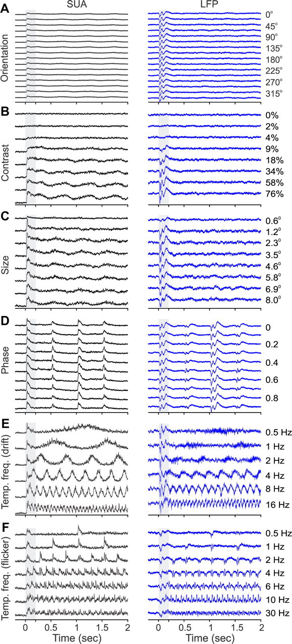
Population analysis summary for SUA/LFP visual response tuning. A population sum of all SUA/LFP PSTHs measured in this study for each response property. A, Orientation (n = 113 recordings). B, Contrast (n = 54 recordings). C, Size (n = 31 recordings). D, Phase (n = 71 recordings). E, Temporal frequency measured with drifting gratings (n = 5 recordings). F, Temporal frequency measured with flickering gratings (n = 10 recordings tested with the same temporal frequency values of 18 measured with flickering gratings).

Discussion

Our results demonstrate that LFP signals in visual cortex are tuned to different response properties, including orientation, direction of movement, contrast, size, spatial phase, and temporal frequency. We show that, although LFP stimulus tuning can be demonstrated at multiple frequency bands, LFP and SUA stimulus preferences are best matched at the high-gamma frequency band during sustained visual stimulation and at lower frequency bands during transient stimulation. We also demonstrate that SUA has better signal-to-noise, contrast sensitivity, and stimulus selectivity than LFP and that different LFP frequencies are associated with different populations of neurons in area V1.

Our results support the notion that high-gamma LFP is restricted to a small population of locally synchronized neurons that share similar response properties in visual cortex (Siegel and König, 2003; Henrie and Shapley, 2005; Niessing et al., 2005). The SUA and LFP stimulus preferences were only matched at the highest frequency bands (beta and gamma) during sustained stimulation, indicating that neurons contributing to high-frequency LFP have to be relatively close to the electrode tip (i.e., the mismatch in the stimulus preferences of single neurons increases with distance in area V1). The poor match at low frequencies during sustained stimulation could have two possible explanations. One explanation is that the cortex acts as a low-pass capacitative filter, allowing low frequencies to travel longer distances than high frequencies (Bédard et al., 2004). Although there is strong evidence that the impedance of the cortical tissue is not frequency dependent (Ranck, 1963; Logothetis et al., 2007), there is a large diversity of axial dendritic resistivity among neurons that could generate the frequency-dependent impedance needed for a low-pass filter (Pettersen and Einevoll, 2008; Lindén et al., 2010). A second possible explanation is that low- and high-frequency LFP originate from different populations of neurons (Logothetis et al., 2007), with neurons having the largest number of thick dendrites generating LFP signals that travel the longest distances (Pettersen and Einevoll, 2008; Lindén et al., 2010). Consistent with this second explanation, the selective stimulation of fast spiking inhibitory neurons has been shown to amplify gamma oscillations, whereas the stimulation of pyramidal neurons amplifies lower frequency oscillations (Cardin et al., 2009). Also, multiunit recordings demonstrated laminar differences in spike-field coherence for low and high frequencies (Buffalo et al., 2011). Our results also support this second explanation by demonstrating that the strength of the spike-field coherence is correlated with the polarity of the LFP. The strongest coherence at low LFP frequencies originated from V1 cells near cortical current sinks, and the strongest coherence at gamma frequencies originated from V1 cells near cortical current sources. In addition, we demonstrate that the strength of the spike-field coherence depends on the response properties of the V1 neurons: low LFP frequencies are associated with V1 cells with nonlinear spatial summation and poor orientation/direction selectivity, whereas gamma frequency coherence is associated with V1 cells with more diverse response properties.

Differences in response selectivity between low- and high-frequency LFP could also be explained if low-frequency LFP originates from larger cortical regions than high-frequency LFP. Consistent with this prediction, our results demonstrate that, during sustained stimulation, the LFP/SUA preferences for stimulus size are correlated at lower frequency bands (>12 Hz) than the preferences for stimulus orientation (>30 Hz), and the preferences for stimulus orientation preferences are correlated at lower frequency bands than the preferences for stimulus phase (>90 Hz; see Table 3). These results are consistent with the finding that the average cortical spread is larger for iso-retinotopy [∼2.5 mm (Albus, 1975)] than for iso-orientation [∼500 μm (Hübener et al., 1997)] and larger for iso-orientation than for iso-spatial phase in the cat [<300 μm (Jin et al., 2008)]. In primates, the cortical spread is also larger for iso-retinotopy than for iso-orientation (Obermayer and Blasdel, 1993), but the cortical spread for spatial phase is unknown (Aronov et al., 2003). Previous studies in inferotemporal cortex also estimated that low-frequency LFP signals (<40 Hz) originate from a region of 3 mm diameter (Kreiman et al., 2006), and in area MT (Liu and Newsome, 2006), LFP speed tuning, which is organized on a spatial scale of 300–600 μm (Liu and Newsome, 2003), was found to deteriorate at higher frequencies than direction tuning, which is organized on a scale of up to 2 mm (Albright et al., 1984; DeAngelis and Newsome, 1999). A significant correlation between gamma LFP and MUA (Berens et al., 2008a,b) was also demonstrated for ocular dominance columns, which are organized on a scale of 500–800 μm (Hubel and Wiesel, 1968; Blasdel, 1992; Obermayer and Blasdel, 1993). It is important to emphasize that, although LFP/SUA stimulus preferences were only correlated at the highest frequency bands during sustained stimulation, during the stimulus transient, we also found correlations at the low-frequency bands. These correlations at low frequencies further support the notion that low- and high-frequency LFPs originate from different populations of neurons (Pettersen and Einevoll, 2008; Cardin et al., 2009; Lindén et al., 2010).

Although the LFP signal is heavily dominated by neuronal synaptic activity (Nunez, 2006; Poulet and Petersen, 2008; Okun et al., 2010; Lindén et al., 2011), it can also contain low-frequency components of spikes. Our results suggest that the contribution from single spikes to LFP tuning is small even at the highest frequency bands that we tested. First, large spikes tuned to a specific stimulus property could be simultaneously recorded with high-gamma LFP that was untuned or showed different tuning to the SUA. Second, the power of the high-gamma LFP was poorly correlated with spike amplitude. Third, we frequently found an excellent match in the LFP/SUA stimulus preferences at the high-gamma band during sustained stimulation but not during transient stimulation, even if the instantaneous spike rate was higher during transient stimulation. Finally, the high-gamma LFP/SUA signals were frequently well matched for some response properties (e.g., orientation preference) but not others (e.g., direction selectivity, orientation bandwidth). The electrodes used in our recordings had sharp tips (∼1 μm tip, ∼15 μm shaft) with a metal exposed area of ∼100–200 μm². It is possible that the match in response properties between SUA and LFP could not be demonstrated if our electrodes had more exposed metal area, because larger tips pool signals from larger cortical regions and frequently fail to isolate single units.

Previous studies demonstrated that gamma LFP is tuned to the stimulus orientation, temporal frequency, and contrast in V1 (Frien et al., 2000; Kayser and König, 2004; Henrie and Shapley, 2005), and LFP has also been found to be spatially tuned in parietal cortex during memory-guided saccades (Pesaran et al., 2002). However, to better understand the neuronal mechanisms underlying LFP selectivity, it is important to measure the selectivity of the neighboring single neurons that are likely to contribute to the LFP signal. This comparison has been performed in extrastriate cortex for speed and direction tuning (Liu and Newsome, 2006), but a detailed comparison in V1 was still missing. Comparisons between LFP and MUA have been obtained in the past (Frien and Eckhorn, 2000; Kreiman et al., 2006; Berens et al., 2008a,b), but it is difficult to estimate the number of neurons contributing to the MUA signal. Therefore, a direct comparison with well isolated neurons (SUA) was needed. The V1 offered a unique opportunity to study this LFP/SUA relation because its neuronal response properties are known with a great level of detail (Hubel and Wiesel, 1968; Gilbert, 1977; DeAngelis et al., 1999; Ringach et al., 2002; Gur et al., 2005). LFP recordings have become an important experimental approach to measure the activity from populations of neurons in the cerebral cortex. However, there are still major questions that remain open about the type and number of neurons that contribute to the LFP signal and the frequency dependency of this contribution. Recent studies suggest that the origin of LFP signals is restricted to a region of 500 μm diameter (Katzner et al., 2009; Xing et al., 2009; Lindén et al., 2011), a cortical spread that can be amplified by correlations among neurons with similar response properties (Lindén et al., 2011). Our work adds to these findings by demonstrating a robust match in the stimulus preference of LFP and single neurons recorded from the same electrode tip, a match that can be explained if the LFP pool signals from neuronal groups with similar stimulus preferences. Based on the size of neuronal domains with similar orientation preference [∼500 μm (Hübener et al., 1997)] and spatial phase [∼300 μm (Jin et al., 2008, 2011)] in cat visual cortex and, assuming that the size of the domains for orientation (Obermayer and Blasdel, 1993) and spatial phase (Aronov et al., 2003) are not much larger in primates, the LFP should pool neurons within a diameter of 500 μm at low-gamma frequency and 300 μm at high-gamma frequency.

References

- Albright TD, Desimone R, Gross CG. Columnar organization of directionally selective cells in visual area MT of the macaque. J Neurophysiol. 1984;51:16–31. doi: 10.1152/jn.1984.51.1.16. [DOI] [PubMed] [Google Scholar]
- Albus K. A quantitative study of the projection area of the central and the paracentral visual field in area 17 of the cat. I. The precision of the topography. Exp Brain Res. 1975;24:159–179. doi: 10.1007/BF00234061. [DOI] [PubMed] [Google Scholar]
- Andersen RA, Musallam S, Pesaran B. Selecting the signals for a brain-machine interface. Curr Opin Neurobiol. 2004;14:720–726. doi: 10.1016/j.conb.2004.10.005. [DOI] [PubMed] [Google Scholar]
- Aronov D, Reich DS, Mechler F, Victor JD. Neural coding of spatial phase in V1 of the macaque monkey. J Neurophysiol. 2003;89:3304–3327. doi: 10.1152/jn.00826.2002. [DOI] [PubMed] [Google Scholar]
- Bédard C, Kröger H, Destexhe A. Modeling extracellular field potentials and the frequency-filtering properties of extracellular space. Biophys J. 2004;86:1829–1842. doi: 10.1016/S0006-3495(04)74250-2. [DOI] [PMC free article] [PubMed] [Google Scholar]
- Berens P, Keliris GA, Ecker AS, Logothetis NK, Tolias AS. Comparing the feature selectivity of the gamma-band of the local field potential and the underlying spiking activity in primate visual cortex. Front Syst Neurosci. 2008a;2:2. doi: 10.3389/neuro.06.002.2008. [DOI] [PMC free article] [PubMed] [Google Scholar]
- Berens P, Keliris GA, Ecker AS, Logothetis NK, Tolias AS. Feature selectivity of the gamma-band of the local field potential in primate primary visual cortex. Front Neurosci. 2008b;2:199–207. doi: 10.3389/neuro.01.037.2008. [DOI] [PMC free article] [PubMed] [Google Scholar]
- Blasdel GG. Orientation selectivity, preference, and continuity in monkey striate cortex. J Neurosci. 1992;12:3139–3161. doi: 10.1523/JNEUROSCI.12-08-03139.1992. [DOI] [PMC free article] [PubMed] [Google Scholar]
- Bokil H, Andrews P, Kulkarni JE, Mehta S, Mitra PP. Chronux: a platform for analyzing neural signals. J Neurosci Methods. 2010;192:146–151. doi: 10.1016/j.jneumeth.2010.06.020. [DOI] [PMC free article] [PubMed] [Google Scholar]
- Bollimunta A, Chen Y, Schroeder CE, Ding M. Neuronal mechanisms of cortical alpha oscillations in awake-behaving macaques. J Neurosci. 2008;28:9976–9988. doi: 10.1523/JNEUROSCI.2699-08.2008. [DOI] [PMC free article] [PubMed] [Google Scholar]
- Bosman CA, Womelsdorf T, Desimone R, Fries P. A microsaccadic rhythm modulates gamma-band synchronization and behavior. J Neurosci. 2009;29:9471–9480. doi: 10.1523/JNEUROSCI.1193-09.2009. [DOI] [PMC free article] [PubMed] [Google Scholar]
- Buffalo EA, Fries P, Landman R, Buschman TJ, Desimone R. Laminar differences in gamma and alpha coherence in the ventral stream. Proc Natl Acad Sci U S A. 2011;108:11262–11267. doi: 10.1073/pnas.1011284108. [DOI] [PMC free article] [PubMed] [Google Scholar]
- Cardin JA, Carlén M, Meletis K, Knoblich U, Zhang F, Deisseroth K, Tsai LH, Moore CI. Driving fast-spiking cells induces gamma rhythm and controls sensory responses. Nature. 2009;459:663–667. doi: 10.1038/nature08002. [DOI] [PMC free article] [PubMed] [Google Scholar]
- Chen Y, Martinez-Conde S, Macknik SL, Bereshpolova Y, Swadlow HA, Alonso JM. Task difficulty modulates the activity of specific neuronal populations in primary visual cortex. Nat Neurosci. 2008;11:974–982. doi: 10.1038/nn.2147. [DOI] [PMC free article] [PubMed] [Google Scholar]
- DeAngelis GC, Newsome WT. Organization of disparity-selective neurons in macaque area MT. J Neurosci. 1999;19:1398–1415. doi: 10.1523/JNEUROSCI.19-04-01398.1999. [DOI] [PMC free article] [PubMed] [Google Scholar]
- DeAngelis GC, Ghose GM, Ohzawa I, Freeman RD. Functional micro-organization of primary visual cortex: receptive field analysis of nearby neurons. J Neurosci. 1999;19:4046–4064. doi: 10.1523/JNEUROSCI.19-10-04046.1999. [DOI] [PMC free article] [PubMed] [Google Scholar]
- Frien A, Eckhorn R. Functional coupling shows stronger stimulus dependency for fast oscillations than for low-frequency components in striate cortex of awake monkey. Eur J Neurosci. 2000;12:1466–1478. doi: 10.1046/j.1460-9568.2000.00026.x. [DOI] [PubMed] [Google Scholar]
- Frien A, Eckhorn R, Bauer R, Woelbern T, Gabriel A. Fast oscillations display sharper orientation tuning than slower components of the same recordings in striate cortex of the awake monkey. Eur J Neurosci. 2000;12:1453–1465. doi: 10.1046/j.1460-9568.2000.00025.x. [DOI] [PubMed] [Google Scholar]
- Fries P, Neuenschwander S, Engel AK, Goebel R, Singer W. Rapid feature selective neuronal synchronization through correlated latency shifting. Nat Neurosci. 2001;4:194–200. doi: 10.1038/84032. [DOI] [PubMed] [Google Scholar]
- Fries P, Womelsdorf T, Oostenveld R, Desimone R. The effects of visual stimulation and selective visual attention on rhythmic neuronal synchronization in macaque area V4. J Neurosci. 2008;28:4823–4835. doi: 10.1523/JNEUROSCI.4499-07.2008. [DOI] [PMC free article] [PubMed] [Google Scholar]
- Gilbert CD. Laminar differences in receptive field properties of cells in cat primary visual cortex. J Physiol. 1977;268:391–421. doi: 10.1113/jphysiol.1977.sp011863. [DOI] [PMC free article] [PubMed] [Google Scholar]
- Gur M, Kagan I, Snodderly DM. Orientation and direction selectivity of neurons in V1 of alert monkeys: functional relationships and laminar distributions. Cereb Cortex. 2005;15:1207–1221. doi: 10.1093/cercor/bhi003. [DOI] [PubMed] [Google Scholar]
- Henrie JA, Shapley R. LFP power spectra in V1 cortex: the graded effect of stimulus contrast. J Neurophysiol. 2005;94:479–490. doi: 10.1152/jn.00919.2004. [DOI] [PubMed] [Google Scholar]
- Hubel DH, Wiesel TN. Receptive fields, binocular interaction and functional architecture in the cat's visual cortex. J Physiol. 1962;160:106–154. doi: 10.1113/jphysiol.1962.sp006837. [DOI] [PMC free article] [PubMed] [Google Scholar]
- Hubel DH, Wiesel TN. Receptive fields and functional architecture of monkey striate cortex. J Physiol. 1968;195:215–243. doi: 10.1113/jphysiol.1968.sp008455. [DOI] [PMC free article] [PubMed] [Google Scholar]
- Hübener M, Shoham D, Grinvald A, Bonhoeffer T. Spatial relationships among three columnar systems in cat area 17. J Neurosci. 1997;17:9270–9284. doi: 10.1523/JNEUROSCI.17-23-09270.1997. [DOI] [PMC free article] [PubMed] [Google Scholar]
- Jin J, Wang Y, Swadlow HA, Alonso JM. Population receptive fields of ON and OFF thalamic inputs to an orientation column in visual cortex. Nat Neurosci. 2011;14:232–238. doi: 10.1038/nn.2729. [DOI] [PubMed] [Google Scholar]
- Jin JZ, Weng C, Yeh CI, Gordon JA, Ruthazer ES, Stryker MP, Swadlow HA, Alonso JM. On and off domains of geniculate afferents in cat primary visual cortex. Nat Neurosci. 2008;11:88–94. doi: 10.1038/nn2029. [DOI] [PMC free article] [PubMed] [Google Scholar]
- Jones JP, Palmer LA. The two-dimensional spatial structure of simple receptive fields in cat striate cortex. J Neurophysiol. 1987;58:1187–1211. doi: 10.1152/jn.1987.58.6.1187. [DOI] [PubMed] [Google Scholar]
- Juergens E, Guettler A, Eckhorn R. Visual stimulation elicits locked and induced gamma oscillations in monkey intracortical- and EEG-potentials, but not in human EEG. Exp Brain Res. 1999;129:247–259. doi: 10.1007/s002210050895. [DOI] [PubMed] [Google Scholar]
- Katzner S, Nauhaus I, Benucci A, Bonin V, Ringach DL, Carandini M. Local origin of field potentials in visual cortex. Neuron. 2009;61:35–41. doi: 10.1016/j.neuron.2008.11.016. [DOI] [PMC free article] [PubMed] [Google Scholar]
- Kayser C, König P. Stimulus locking and feature selectivity prevail in complementary frequency ranges of V1 local field potentials. Eur J Neurosci. 2004;19:485–489. doi: 10.1111/j.0953-816x.2003.03122.x. [DOI] [PubMed] [Google Scholar]
- Keliris GA, Logothetis NK, Tolias AS. The role of the primary visual cortex in perceptual suppression of salient visual stimuli. J Neurosci. 2010;30:12353–12365. doi: 10.1523/JNEUROSCI.0677-10.2010. [DOI] [PMC free article] [PubMed] [Google Scholar]
- Kreiman G, Hung CP, Kraskov A, Quiroga RQ, Poggio T, DiCarlo JJ. Object selectivity of local field potentials and spikes in the macaque inferior temporal cortex. Neuron. 2006;49:433–445. doi: 10.1016/j.neuron.2005.12.019. [DOI] [PubMed] [Google Scholar]
- Lindén H, Pettersen KH, Einevoll GT. Intrinsic dendritic filtering gives low-pass power spectra of local field potentials. J Comput Neurosci. 2010;29:423–444. doi: 10.1007/s10827-010-0245-4. [DOI] [PubMed] [Google Scholar]
- Lindén H, Tetzlaff T, Potjans TC, Pettersen KH, Grün S, Diesmann M, Einevoll GT. Modeling the spatial reach of the LFP. Neuron. 2011;72:859–872. doi: 10.1016/j.neuron.2011.11.006. [DOI] [PubMed] [Google Scholar]
- Liu J, Newsome WT. Functional organization of speed tuned neurons in visual area MT. J Neurophysiol. 2003;89:246–256. doi: 10.1152/jn.00097.2002. [DOI] [PubMed] [Google Scholar]
- Liu J, Newsome WT. Local field potential in cortical area MT: stimulus tuning and behavioral correlations. J Neurosci. 2006;26:7779–7790. doi: 10.1523/JNEUROSCI.5052-05.2006. [DOI] [PMC free article] [PubMed] [Google Scholar]
- Logothetis NK, Kayser C, Oeltermann A. In vivo measurement of cortical impedance spectrum in monkeys: implications for signal propagation. Neuron. 2007;55:809–823. doi: 10.1016/j.neuron.2007.07.027. [DOI] [PubMed] [Google Scholar]
- Mitzdorf U. Current source-density method and application in cat cerebral cortex: investigation of evoked potentials and EEG phenomena. Physiol Rev. 1985;65:37–100. doi: 10.1152/physrev.1985.65.1.37. [DOI] [PubMed] [Google Scholar]
- Naka KI, Rushton WA. S-potentials from luminosity units in the retina of fish (Cyprinidae) J Physiol. 1966;185:587–599. doi: 10.1113/jphysiol.1966.sp008003. [DOI] [PMC free article] [PubMed] [Google Scholar]
- Niessing J, Ebisch B, Schmidt KE, Niessing M, Singer W, Galuske RA. Hemodynamic signals correlate tightly with synchronized gamma oscillations. Science. 2005;309:948–951. doi: 10.1126/science.1110948. [DOI] [PubMed] [Google Scholar]
- Nunez PL. Electric fields of the brain: the neurophysics of EEG. Oxford: Oxford UP; 2006. [Google Scholar]
- Obermayer K, Blasdel GG. Geometry of orientation and ocular dominance columns in monkey striate cortex. J Neurosci. 1993;13:4114–4129. doi: 10.1523/JNEUROSCI.13-10-04114.1993. [DOI] [PMC free article] [PubMed] [Google Scholar]
- Okun M, Naim A, Lampl I. The subthreshold relation between cortical local field potential and neuronal firing unveiled by intracellular recordings in awake rats. J Neurosci. 2010;30:4440–4448. doi: 10.1523/JNEUROSCI.5062-09.2010. [DOI] [PMC free article] [PubMed] [Google Scholar]
- Peirce JW. The potential importance of saturating and supersaturating contrast response functions in visual cortex. J Vis. 2007;7:13. doi: 10.1167/7.6.13. [DOI] [PMC free article] [PubMed] [Google Scholar]
- Pesaran B, Pezaris JS, Sahani M, Mitra PP, Andersen RA. Temporal structure in neuronal activity during working memory in macaque parietal cortex. Nat Neurosci. 2002;5:805–811. doi: 10.1038/nn890. [DOI] [PubMed] [Google Scholar]
- Pettersen KH, Einevoll GT. Amplitude variability and extracellular low-pass filtering of neuronal spikes. Biophys J. 2008;94:784–802. doi: 10.1529/biophysj.107.111179. [DOI] [PMC free article] [PubMed] [Google Scholar]
- Poulet JF, Petersen CC. Internal brain state regulates membrane potential synchrony in barrel cortex of behaving mice. Nature. 2008;454:881–885. doi: 10.1038/nature07150. [DOI] [PubMed] [Google Scholar]
- Ranck JB., Jr Specific impedance of rabbit cerebral cortex. Exp Neurol. 1963;7:144–152. doi: 10.1016/s0014-4886(63)80005-9. [DOI] [PubMed] [Google Scholar]
- Ringach DL, Sapiro G, Shapley R. A subspace reverse-correlation technique for the study of visual neurons. Vis Res. 1997;37:2455–2464. doi: 10.1016/s0042-6989(96)00247-7. [DOI] [PubMed] [Google Scholar]
- Ringach DL, Shapley RM, Hawken MJ. Orientation selectivity in macaque V1: diversity and laminar dependence. J Neurosci. 2002;22:5639–5651. doi: 10.1523/JNEUROSCI.22-13-05639.2002. [DOI] [PMC free article] [PubMed] [Google Scholar]
- Siegel M, König P. A functional gamma-band defined by stimulus-dependent synchronization in area 18 of awake behaving cats. J Neurosci. 2003;23:4251–4260. doi: 10.1523/JNEUROSCI.23-10-04251.2003. [DOI] [PMC free article] [PubMed] [Google Scholar]
- Skottun BC, De Valois RL, Grosof DH, Movshon JA, Albrecht DG, Bonds AB. Classifying simple and complex cells on the basis of response modulation. Vis Res. 1991;31:1079–1086. doi: 10.1016/0042-6989(91)90033-2. [DOI] [PubMed] [Google Scholar]
- Stoelzel CR, Bereshpolova Y, Swadlow HA. Stability of thalamocortical synaptic transmission across awake brain states. J Neurosci. 2009;29:6851–6859. doi: 10.1523/JNEUROSCI.5983-08.2009. [DOI] [PMC free article] [PubMed] [Google Scholar]
- Swadlow HA, Gusev AG, Bezdudnaya T. Activation of a cortical column by a thalamocortical impulse. J Neurosci. 2002;22:7766–7773. doi: 10.1523/JNEUROSCI.22-17-07766.2002. [DOI] [PMC free article] [PubMed] [Google Scholar]
- Swadlow HA, Bereshpolova Y, Bezdudnaya T, Cano M, Stoelzel CR. A multi-channel, implantable microdrive system for use with sharp, ultra-fine “Reitboeck” microelectrodes. J Neurophysiol. 2005;93:2959–2965. doi: 10.1152/jn.01141.2004. [DOI] [PubMed] [Google Scholar]
- Swindale NV, Grinvald A, Shmuel A. The spatial pattern of response magnitude and selectivity for orientation and direction in cat visual cortex. Cereb Cortex. 2003;13:225–238. doi: 10.1093/cercor/13.3.225. [DOI] [PubMed] [Google Scholar]
- Xing D, Yeh CI, Shapley RM. Spatial spread of the local field potential and its laminar variation in visual cortex. J Neurosci. 2009;29:11540–11549. doi: 10.1523/JNEUROSCI.2573-09.2009. [DOI] [PMC free article] [PubMed] [Google Scholar]
- Zanos TP, Mineault PJ, Pack CC. Removal of spurious correlations between spikes and local field potentials. J Neurophysiol. 2011;105:474–486. doi: 10.1152/jn.00642.2010. [DOI] [PubMed] [Google Scholar]