Network inference using steady-state data and Goldbeter–koshland kinetics

Abstract

Motivation: Network inference approaches are widely used to shed light on regulatory interplay between molecular players such as genes and proteins. Biochemical processes underlying networks of interest (e.g. gene regulatory or protein signalling networks) are generally nonlinear. In many settings, knowledge is available concerning relevant chemical kinetics. However, existing network inference methods for continuous, steady-state data are typically rooted in statistical formulations, which do not exploit chemical kinetics to guide inference.

Results: Herein, we present an approach to network inference for steady-state data that is rooted in non-linear descriptions of biochemical mechanism. We use equilibrium analysis of chemical kinetics to obtain functional forms that are in turn used to infer networks using steady-state data. The approach we propose is directly applicable to conventional steady-state gene expression or proteomic data and does not require knowledge of either network topology or any kinetic parameters. We illustrate the approach in the context of protein phosphorylation networks, using data simulated from a recent mechanistic model and proteomic data from cancer cell lines. In the former, the true network is known and used for assessment, whereas in the latter, results are compared against known biochemistry. We find that the proposed methodology is more effective at estimating network topology than methods based on linear models.

Availability: mukherjeelab.nki.nl/CODE/GK_Kinetics.zip

Contact: c.j.oates@warwick.ac.uk; s.mukherjee@nki.nl

Supplementary Information: Supplementary data are available at Bioinformatics online.

1 INTRODUCTION

Networks of molecular components play a prominent role in molecular and systems biology. A graph G = (V(G), E(G)) can be used to describe a biological network, with vertex set V(G) identified with molecular components (e.g. genes or proteins) and edge set E(G) with regulatory interplay between the components. Edges in a biological network are often associated with the causal notion that intervention on a parent node influences its child node(s). Data-driven characterization of the graph structure E(G) (often referred to as the topology) is known as network inference and has emerged as an important problem class in bioinformatics and systems biology. Network inference can aid in efficient generation of biological hypotheses from high-throughput data. Further, network inference can aid in exploring molecular interplay that is associated with specific phenotypes, such as disease states.

From a statistical perspective, network inference entails reverse-engineering a graph G using biochemical data and, where available, prior knowledge regarding aspects of the topology. Over the last decade, many methods for network inference have been proposed (see e.g. Lee and Tzou, 2009; Markowetz and Spang, 2007). To date, most methods for network inference have been rooted in discrete or linear formulations (Bender et al., 2010; Hill, 2012; Morrissey et al., 2010; Opgen-Rhein and Strimmer, 2007; Sachs et al., 2005). As discussed in Oates and Mukherjee (2012a), a wide range of existing approaches can be viewed as variants of the statistical linear model (‘linear’ refers to linearity in parameters, so that nonlinear basis functions may be used within a ‘linear’ framework). Moreover, a number of approaches based on ordinary differential equations (ODEs; Bansal et al., 2007; Nam et al., 2007) are ultimately reducible to linear statistical models, as described in Oates et al. (2012).

However, the biochemical processes underlying biological networks are often highly non-linear. When the data-generating process is non-linear, use of linear models may produce inefficient or inconsistent estimation, attributing causal status to artifacts resulting from model misspecification (Heagerty and Kurland, 2001; Lv and Liu, 2010). Indeed, such bias can prevent recovery of the correct network even in favourable asymptotic limits of large sample size and low noise (Oates and Mukherjee, 2012a). On the other hand, in many settings, non-linear dynamical models of relevant biochemical processes are available. For example, gene regulation may be modelled using Michaelis–Menten functionals (Cantone et al., 2009), and metabolism may be modelled using mass action chemical kinetics (Lee et al., 2008). Here, we describe an approach by which kinetic models can be used to inform network inference from steady-state data. As we show below, such information can be valuable in guiding exploration of network topologies.

Kinetic formulations have been widely studied in the systems biology literature, and recently, there has been much interest in statistical inference for such systems (e.g. Chen et al., 2009; Xu et al., 2010). Our work is in a similar vein but focuses on network inference per se and on the steady-state rather than time-course setting. Although biochemical assays have become cheaper, it remains the case that experimental designs must often negotiate a trade off between more conditions (e.g. perturbations, biological samples and technical replicates) and temporal resolution. Methodologies, which can exploit knowledge concerning relevant dynamical systems in the steady-state setting, are therefore potentially valuable.

In brief, we proceed as follows. We consider a class of non-linear biochemical dynamical systems that are relevant to the biological process of interest (we focus on protein signalling, discussed in detail later). Steady-state analysis leads to a class of functional relationships between parent and child. These functional relationships are used to formulate a statistical model for network inference from steady-state data. In this way, network inference is rooted in functional relationships derived from non-linear kinetics. Importantly, we do not assume detailed knowledge of the dynamical system, but only the broad class to which dynamics and associated equilibria may belong. Indeed, the approach we describe does not require any kinetic parameters to be known a priori nor knowledge of the network topology and is in that sense directly comparable with conventional network inference methods. Its potential advantage stems from then rich yet constrained nature of the class of functional relationships that are considered. As recently discussed in Peters et al. (2011), non-linear functional forms can aid in identification of underlying causal relationships.

We develop these ideas in the context of protein signalling mediated by phosphorylation. Enzyme kinetics have been extensively studied, and dynamical formulations are widely available in the literature (see e.g. Leskovac, 2003). For some proteins and pathways, regulation has been studied in considerable causal and mechanistic detail. Indeed, there exist detailed computational models for canonical protein signalling pathways, which have been validated against experimental data (e.g. Schoeberl et al., 2002; Xu et al., 2010). Further, proteomic technologies now allow multivariate, data-driven study of phosphorylation, facilitating biological validation of network inference methodologies. We take advantage of these factors to examine the performance of our approach using both simulated and real data.

In the phosphorylation setting, Goldbeter–Koshland kinetics (Goldbeter and Koshland, 1981) form the functional class that underlies our network inference approach. Goldbeter–Koshland kinetics are well known to be capable of highly non-linear behaviour including exquisite sensitivity. It has been experimentally demonstrated that this so-called ultrasensitivity is biologically relevant to signalling network dynamics, facilitating abrupt and precise decision making (e.g Kim and Ferrell, 2007). We carry out statistical inference in a Bayesian framework, using reversible-jump Markov chain Monte Carlo (RJMCMC) to explore the joint model and parameter space. This yields posterior probability scores for edges in the network that are analogous to scores obtained in existing statistical network inference approaches for steady-state data (Ellis and Wong, 2008; Mukherjee and Speed, 2008).

The remainder of this article is organized as follows. In Section 2, our approach is laid out, followed by an exposition of the associated computational statistics. In Section 3, we present results on data simulated from a recently developed dynamical model of the mitogen-activated protein kinase (MAPK) signalling that has been validated against experimental data (Xu et al., 2010). We then show results on real proteomic data from breast cancer cell lines. Finally, Section 4 closes with a discussion of practical implications and opportunities for network inference based on functional models, along with associated technical challenges.

2 METHODS

We begin in Section 2.1 by describing our approach in general terms. Section 2.2 then introduces relevant concepts in the application area of protein phosphorylation. In particular, we describe a class of non-linear equations derived from Goldbeter–Koshland kinetics. Next, in Section 2.3, this model class is embedded into a Bayesian statistical framework for observations obtained at equilibrium. Inference over model space is facilitated by reversible-jump MCMC, with Section 2.4 dedicated to a presentation of our sampling scheme and a discussion of key implementational details.

2.1 General formulation

We consider a state vector 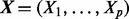containing concentrations of p proteins. Equilibrium analysis of phosphorylation dynamics, as described below, leads to a system of p equations 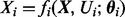where i indexes proteins, U_i are external input variables and θ_i unknown parameters. The component function f_i depends on a subset π_i of the state variables, such that we may write , where indicates selection of components of the vector X whose indices are members of the set π_i. Variables j∈π_i are the parents of node i in graph G; the parent sets π_i specify the (unknown) topology of interest since (j,i)∈E(G)⇔j∈π_i. Our inference scheme seeks to infer the π_i's from steady-state data. Since the dynamical system is not usually known in detail a priori, we consider the practically applicable case in which the f_i's are known only to belong to a certain class (derived from Goldbeter–Koshland kinetics, as described below) with parent sets π_i and all parameters θ_i remaining unknown.

2.2 Protein phosphorylation

We consider proteins , each of which has an unphosphorylated form and a phosphorylated form X_i (i∈V). Phosphorylated proteins are referred to as phosphoproteins. The chemical reaction that gives product X_i from substrate is known as phosphorylation and is catalysed by kinases X_E (). We consider the case in which the kinases themselves are phosphoproteins (if phosphorylation is not driven by a kinase in V, we set ). The ability of a kinase to catalyse phosphorylation of X_i may be tempered by inhibitors X_I (; the double subscript indicates that inhibition is specific to both substrate and kinase). Thus the parents π_i of X_i comprise both the kinases and their inhibitors: 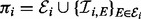. Because of specificity of phosphorylation reactions, we assume that the underlying network G is sparse, such that the number of parents π_i for variate X_i is low. An example is shown, using a standard graphical representation, in Figure 1a. In what follows we use to denote the concentrations of proteins , respectively; is then the total concentration of protein i, which is taken to be approximately invariant over the timescale of phosphorylation dynamics.

Fig. 1.

Overview of approach. (a) An example of a phosphorylation network. (b) Our approach couples automatic generation of chemical models with Bayesian model selection to infer regulators π_i of species i. (c) A statistical formulation (graphical model) for equilibrium phosphorylation of species i is characterized by specifying kinases () and inhibitors () of kinases. [Bounding boxes are used to indicate multiplicity of variables, shaded nodes are observed with noise.]

For network inference, model selection will take place over parent sets π_i. Accordingly, we require functional equations for any such subset (Fig. 1b). We use ODEs of the Michaelis–Menten type to provide a suitable class of analytic approximations for phosphorylation dynamics (Kholodenko, 2006; Steijaert et al., 2010). The rate of phosphorylation due to kinase X_j is given by 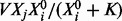, which explicitly acknowledges variation of kinase concentration X_j and permits kinase-specific response profiles (parameterized by K) with maximum reaction rate V.

Equilibrium analysis of the foregoing kinetic model yields functional relationships between nodes that we use to inform analysis of steady-state data. The seminal example of Goldbeter and Koshland (1981) considered phosphorylation by a single enzyme (X_E) and dephosphorylation by a single phosphatase (X_P), which at equilibrium satisfy the balance equation

(1)

whose solution 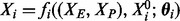is capable of expressing a range of biologically relevant non-linearities. In this work, we extend the class of molecular regulatory mechanisms by entertaining multiple kinases along with multiple kinase inhibitors. For simplicity, we assert that all kinases act independently and that all kinase inhibition occurs competitively. In particular we do not consider complex interactions between these regulators, such as cooperativity. Competitive inhibition requires that substrate () and inhibitor (X_I) compete for the same binding site on the enzyme (X_E):

(2)

When multiple inhibitors () are present, they are assumed to act exclusively, competing for the same binding site on the enzyme:

(3)

Mathematically, competitive inhibition by exclusive inhibitors corresponds to rescaling of the Michaelis–Menten parameter

(4)

where the sum runs over inhibitors I of the kinase E. (The interested reader is referred to Leskovac (2003) for further details.) Phosphatase specificity is currently poorly characterized compared with kinase specificity, so our analysis does not attempt to cover this level of regulation. In particular dephosphorylation is assumed to occur at a rate V₀X_i proportional to the amount of phosphoprotein. Collecting together our modelling assumptions and solving the resulting balance equation produces a functional model class , with member functions given by

(5)

Here, the parameter vector contains the maximum rates (V) and Michaelis–Menten constants (K) specific to phosphorylation of species i (dependence of V, K on i is notationally suppressed for clarity). When we instead define f_i = μ_i, equal to the average phosphoprotein concentration.

2.3 Statistical formulation

The Goldbeter–Koshland model (5) gives a general form for the functional relationship between nodes at steady-state. Inference proceeds based on a Bayesian formulation of this model (Fig. 1c). Consider independent observations of protein expression obtained at equilibrium with respect to phosphorylation dynamics. To fix a characteristic scale, all data are scale normalized prior to inference, such that each species has unit mean. For a given protein i, a model M_i for phosphorylation describes putative kinases and associated inhibitors () for protein i (note that M_i contains more information than the subset π_i, namely the specific mechanistic roles played by each variable in π_i). Then, conditional on M_i and parameters θ_i we have the following statistical model

(6)

where . Here, the error term ε_i absorbs contributions from observation error and model misspecification, with the logarithm of both predictor and response taken to improve the normality assumption.

In the Bayesian setting, prior probability distributions are required for parameters θ_i and models M_i. For the parameters 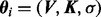, which we have augmented with σ (as with the other parameters, we drop the subscript i on σ for clarity), physical considerations require that V_j, K_j, σ > 0. Following Xu et al. (2010), we postulate that all biological processes must occur on an observable timescale, motivating, in the shape, scale parametrization, the gamma priors V ∼ Γ(2,1/2), K ∼ Γ(2, 1/2), each of unit mean and variance 1/2. The noise parameter σ is inverse-gamma distributed a priori as σ ∼ Γ^-1(6,1), with prior mean 1/5 and variance 1/100 chosen to correspond to the magnitude of measurement noise in current proteomic technologies (Hennessey et al., 2010).

When expert opinion is available, rich subjective model priors may be elicited (see e.g. for graphical models, Mukherjee and Speed, 2008), but for this work we employed an objective prior, depending on a (possibly empty) prior model . Prior specification should account for the distinct roles of kinases and inhibitors; a mathematical formulation is described in the Supplementary Information.

2.4 Reversible jump Markov chain Monte Carlo

Inference over networks was carried out using Markov chain Monte Carlo (MCMC). For linear and discrete models, marginal likelihoods are typically available in closed form. Then, sampling needs only to explore the model space (see e.g. Ellis and Wong, 2008; Madigan et al., 1995; Mukherjee and Speed, 2008). However, in the present, non-linear setting parameters cannot be integrated out analytically, motivating the need to sample over the joint space of models and parameters. Furthermore, the dimension of the model is not fixed, as the number of parameters depends on the model M; where the former quantities are functions of the numbers of kinases and inhibitors according to M. We therefore employ reversible-jump MCMC (RJMCMC) (Green, 1995) for inference. Following Green and Hastie (2009), we enumerate all possible models as and define the across-model state space

(7)

where parameters θ^M(k) for model M^(k) belong to Θ_k and × denotes the Cartesian product. The reversible-jump sampler constructs an ergodic Markov chain on which has, as its stationary distribution, the posterior probability distribution . In particular the marginal over the model index corresponds exactly to the posterior model probabilities . Construction of an efficient RJMCMC sampler requires an intuition for the across-model state space. We adopt a deliberately transparent Metropolis-within-Gibbs approach (Roberts and Rosenthal, 2006), updating one coordinate of at a time using a Metropolis–Hastings accept/reject probability of the form . A number of distinct proposal mechanisms were employed to ensure ergodicity and provide rapid mixing. Precise details of the proposals used, along with their associated ratios may be found in the Supplementary Information. For applications, 30 000 iterations of the Gibbs sampler were performed, with 5000 discarded as burn-in. Convergence was assessed using repeated runs from dispersed initial conditions.

3 RESULTS

In this section, we empirically assess our methodology and compare its performance against network inference based on the linear model. In Section 3.1, we show results using a recently published dynamical model of the MAPK signalling pathway due to Xu et al. (2010), where the underlying network is known exactly. In Section 3.2, we apply our approach to a real proteomic dataset. In both cases, for fair comparison between different methods, no informative model priors were used (i.e. we set ).

3.1 Simulation study

Data were generated from a computational model of the MAPK signaling pathway due to Xu et al. (2010), specified by a system of 25 non-linear ODEs (Fig. 2a). The simulation gives covariates that are highly correlated at equilibrium, as would be expected in practice, while providing a known network G for evaluation purposes. Further details regarding the computational model are described in the Supplementary Information. We introduced independent Gaussian measurement noise, additive on the log scale, of magnitude σ = 0.2, similar to error incurred by current proteomic technologies (Hennessey et al., 2010).

Fig. 2.

Simulation study. (a) Computational model of the MAPK signalling pathway (due to Xu et al., 2010). Circles represent proteins, and rectangles represent interventions (drug treatments) used to perturb the system. For proteins, one strike-through represents inactivity, and two strikes represent degradation. (b) Average receiver operating characteristic (ROC) curves (sample size n = 24, noise σ = 0.2, see text for details) using data generated from model (a). (c) Area under ROC curve (AUR) for each of the sample size (n) and noise (σ) regimes shown (boxplots over 10 datasets for each n, σ regime). ‘G.K. Kinetics’ network inference using Goldbeter–Koshland kinetics as described in text; ‘Lin. Bayes’ Bayesian variable selection using linear model; ‘Lin. Lasso’’ variable selection using LASSO and linear model; ‘Lin. Bayes Adj.’ and ‘Lin. Lasso Adj.’ as previous but corrected for total protein levels as described in text.

We benchmarked our approach against the linear-additive-Gaussian formulation with design matrix and intercept β₀; the logarithm of a vector is taken component wise. All variables were mean-variance standardized prior to inference. We consider two standard approaches to inference for the linear model, namely (i) the LASSO with penalty parameter set according to cross validation (‘Lin. Lasso’) and (ii) a conjugate Bayesian formulation [‘Lin. Bayes’; Hill (2012)], based on the g-prior , with a flat prior over the intercept p(β₀)∝1 and reference prior over the noise p(σ)∝1/σ. For the Bayesian approach, we took a model prior p(M) to be uniform over in-degree with the restriction . Model averaging was then used to obtain posterior inclusion probabilities. For each of the linear approaches (i) and (ii) we also considered adjusted variants (‘Lin. Lasso Adj.’ and ‘Lin. Bayes Adj.’) where log-phospho-ratios constitute the response; this can be motivated as a simple first order correction for variation in total protein levels.

For each phosphorylated or active species i in the computational model, we sought to infer the parents π_i. For a fair comparison with the linear approaches, which do not ascribe functional roles to variables, we did not distinguish between kinases and inhibitors during assessment. The resulting receiver operating characteristic (ROC) curves are shown in Figure 2b. Overall performance was quantified using area under the ROC curve (AUR), aggregated over all i∈V. Results are shown over 10 datasets for each of various combinations of sample size n and noise level σ (Fig. 2c). In all regimes, our approach outperformed linear approaches; the latter did not perform well even in this low dimensional example. We note also that even in the least challenging regime (n = 24, σ = 0), none of the approaches were able to perfectly recover the entire network G. The adjusted regressions, which model the log-phospho-ratio as the response, did not outperform the standard linear regressions.

3.2 Cancer proteomic data

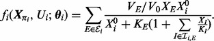
Data were obtained using reverse-phase protein arrays [RPPA; Hennessey et al. (2010)] applied to a panel of breast cancer cell lines (Neve et al., 2006). Data comprised equilibrium observations for p = 38 phosphorylated proteins, in addition to their unphosphoryated counterparts (Fig. 3a). Cell lines belong to two biologically distinct subtypes known as basal (n = 22) and luminal (n = 21), with each member cell line comprising one sample. The true data-generating network is not known for biological samples, but for certain nodes, the relevant kinase–substrate relationships have been described in considerable mechanistic detail in the literature. To minimize the risk of comparing results of inference against an incorrect literature model, we focused attention on selected nodes in the data for each of whom the key kinase is well established. For example, the protein S6 is known to be phosphorylated via the kinase activity of p70 S6 Kinase (p70S6K); both proteins are included in our assay. Treating S6 as the target (i.e. the network child), we scored each of the remaining 37 proteins as a candidate regulator (i.e. for inclusion in the parent set π_S6) using each method. Figure 3b displays the result of inference for the parents of S6 (S6 is phosphorylated on amino acid residues Serine 235 236; results for basal subtype shown and measurements of S6 phosphorylation on residues Serine 240 244 were excluded since this correlates closely with phosphorylation on Serine 235 236). Despite the known well-established regulatory role for p70S6K, it is striking that only our approach ranks p70S6K highly. The LASSO approaches ascribe no weight to the correct kinase in this case. To gain more insight into the assignment of weights by the competing methodologies, we constructed scatter plots comparing weight distributions (Fig. 3c). It is immediately clear that the weight assignments vary markedly between basal and luminal subtypes. In addition, it is noticeable that there is little agreement between the apparently similar linear formulations. We extended this investigation to several other key signalling players whose regulation is well understood (Table 1). Overall, we find that the proposed approach outperforms the linear methods.

Fig. 3.

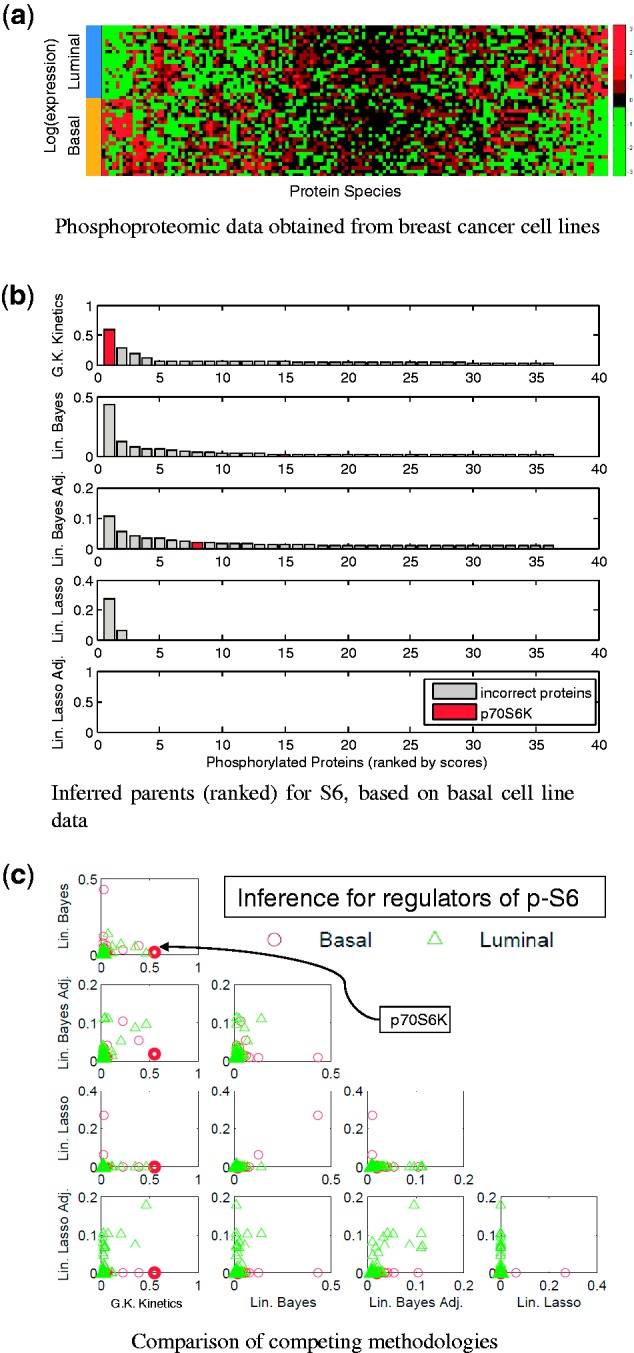
Cancer protein data. (a) Heatmap of reverse-phase protein array data from a panel of breast cancer cell lines. (b) Proteins were ranked as potential regulators of the node S6 under each methodology. The protein p70 S6 Kinase (p70S6K) is known to be a key kinase for the node S6; this known regulator is shown in red in the bar plots. (c) Comparison of methodologies: Each point in the scatter plots represents one phosphoprotein, with the known kinase p70S6K highlighted in bold. [(b) and (c) display weights (posterior probabilities or absolute regression coefficients) assigned to each protein by each method.]

Table 1.

Cancer protein data, comparison of methods

Target	Akt	p70S6K	S6	p53
G.K. Kinetics	4	3	1	8
Lin. Bayes	10	9	15	32
Lin. Bayes Adj.	14	8	8	14
Lin. Lasso	NA	8	NA	NA
Lin. Lasso Adj.	NA	12	NA	NA
Total No of candidates	36	37	36	37

The proposed method was compared with linear approaches using reverse-phase protein array data for nodes whose regulation has been extensively studied in the literature. Each method ranked potential regulators among candidate proteins; here, we display the rank assigned to the known kinase, using each of the five methods. For example, Figure 3b shows such an analysis for the target node (i.e. network child) S6, where G.K. Kinetics ranked the known kinase p70S6K 1st out of a total of 36 candidates. High rank indicates that the known kinase is correctly highlighted in the analysis; the highest-ranked result is highlighted in bold for each target node. Here, we show the rank assigned to the known kinase for each of the target nodes Akt, p70S6k, S6 and p53. (‘NA’ indicates that the known kinase received zero weight. Alternative phospho-forms of the target were excluded as candidates for Akt and S6, so that there were 36 candidates rather than 37. Here, we present results obtained using data from cell lines of basal subtype; luminal results are shown in Supplementary Information.)

4 DISCUSSION AND CONCLUSIONS

In this work, we investigated integration of biochemical mechanisms into network inference for steady-state data. We focused on protein phosphorylation, a key biochemical process where the availability of relatively sophisticated simulation models, extent of existing mechanistic insight and availability of relevant proteomic data combine to facilitate assessment of network inference approaches. Our results, on simulated and real data, demonstrated that protein signalling network topology may be estimated more successfully under our approach than by conventional linear formulations. The linear approaches we used were outperformed on simulated data and failed to identify known regulation in real data. In addition to superior performance, a chemical formulation ascribes mechanistic roles to variables and may increase interpretability. In complementary work, Oates and Mukherjee (2012b) consider the use of nonlinear chemical kinetics for network inference using time-course data, reporting that a chemical formulation outperformed a number of mechanism-free approaches, including non-parametric models.

Estimation of dynamical parameters in the presence of structural uncertainty remains an open area and an important topic for future work. Here, although we sampled both networks and parameters jointly, we focused exclusively on network inference. It remains unclear how to report kinetic parameter estimates in the presence of structural uncertainty. One approach would be to first fix a network and subsequently estimate the associated dynamics. However, this has the disadvantage of relying on a ‘point estimate’ of the network and therefore being sensitive to network misspecification. This is especially relevant in the small sample setting where typically no one model will capture substantial posterior mass. Alternatively, one could estimate the total effect of an interaction by averaging over all models. This relates to ideas in causal inference for graphical models (Pearl, 2009) but has the disadvantage that the resulting ‘total effect’ may lack a natural chemical interpretation.

It is important to note that the chemical formulations considered here are not fully identifiable with respect to parameters. Indeed, the maximal reaction rates V_E are identifiable only up to an unknown normalizing constant V₀, whereas the Michaelis–Menten parameters K_E are known to be only weakly identifiable (Calderhead and Girolami, 2011). Nevertheless, the model structure M itself remains identifiable in this setting (Supplementary Information). Our empirical results on simulated and real data provide examples where structural inference, using the formulation we propose, is possible under realistic conditions. However, factors including model mis-specification and missing variables (see e.g. Oates and Mukherjee, 2012a) may limit structural identifiability in general. Indeed, we found that all approaches performed poorly on luminal cell lines in our real proteomic data example (Supplementary Information). Therefore, results of structural inference should be interpreted with caution and treated as hypotheses to be tested experimentally.

We did not consider an explicit observation model. Because of the nonlinear nature of the Goldbeter–Koshland formulation, formal uncertainty propagation would be highly nontrivial for our model. Assuming log-normal observation error and neglecting predictor uncertainty, we arrived at the statistical model in Equation (6). In this sense, our formulation may be regarded as an approximation to inference under an explicit log-normal observation model. An interesting avenue for further research would be to make explicit the observation process.

Network inference is naturally facilitated by interventional experiments; however, adequate modelling of the effects of intervention is important to ameliorate statistical confounding (Eaton and Murphy, 2007; Pearl, 2009). Within a chemical kinetic framework, such factors may be naturally accounted for; for instance, a ‘perfect’ intervention simply corresponds to removal of the targeted species from the chemical model.

Network inference based on non-linear models is computationally challenging. We considered low-to-moderate dimensional settings (p = 12, 38), for which RJMCMC proved to be effective. The computations in this article are parallelizable, and it may therefore be possible to extend this work to the high-dimensional setting. In general, non-linear approaches are clearly more burdensome than their linear counterparts, where highly efficient approaches, including those based on LASSO and related penalized likelihood schemes, allow rapid estimation even in high dimensions. We therefore view the methods presented here as complementary to variable selection based on linear models, allowing more refined exploration in settings where some insight into underlying dynamics is available.

We investigated integration of biochemical mechanisms into network inference. Although the Goldbeter–Koshland formulae are invalid at the single-cell level, which is intrinsically stochastic, our results suggest that these deterministic non-linear equations represent a better approximation than the corresponding linear equations. In particular a chemical kinetic formulation is able to account, in a principled way, for variation in total protein levels between samples. Consequently, inferred edges cannot be interpreted as indicators of direct biochemical interaction; rather an edge corresponds to the prediction that intervention on the parent will result in a change in expression of the child, possibly indirectly via unobserved variables. In our real data example, we therefore allowed for candidate species, which are not themselves kinases, such as S6 and p53.

For simplicity, we did not consider post-translational modifications such as ubiquitinylation, nor spatial effects such as translocation, nor did we explicitly distinguish between phosphorylation on different residues. The methodology that we presented may be generalized to other molecular mechanisms. In particular alternative mechanisms of enzyme interaction such as non-competitive, uncompetitive, hyperbolic and parabolic inhibition could be readily integrated into our framework.

REFERENCES

- Bansal M, et al. How to infer gene networks from expression profiles. Mol. Syst. Biol. 2007;3:78. doi: 10.1038/msb4100120. [DOI] [PMC free article] [PubMed] [Google Scholar]
- Bender C, et al. Dynamic deterministic effects propagation networks: learning signalling pathways from longitudinal protein array data. Bioinformatics. 2010;26(ECCB 2010):i596–i602. doi: 10.1093/bioinformatics/btq385. [DOI] [PMC free article] [PubMed] [Google Scholar]
- Calderhead B, Girolami M. Statistical analysis of nonlinear dynamical systems using differential geometric sampling methods. J. Roy. Soc. Interface. 2011;1:821–835. doi: 10.1098/rsfs.2011.0051. [DOI] [PMC free article] [PubMed] [Google Scholar]
- Cantone I, et al. A yeast synthetic network for in vivo assessment of reverse-engineering and modeling approaches. Cell. 2009;137:172–181. doi: 10.1016/j.cell.2009.01.055. [DOI] [PubMed] [Google Scholar]
- Chen W, et al. Input-output behavior of ErbB signaling pathways as revealed by a mass action model trained against dynamic data. Mol. Syst. Biol. 2009;5:239. doi: 10.1038/msb.2008.74. [DOI] [PMC free article] [PubMed] [Google Scholar]
- Eaton D, Murphy K. Exact Bayesian structure learning from uncertain interventions. Proceedings of the Eleventh Conference on Artificial Intelligence and Statistics (AISTATS-07) 2007 San Juan, Puerto Rico. [Google Scholar]
- Ellis B, Wong WH. Learning causal Bayesian network structures from experimental data. J. Am. Stat. Assoc. 2008;103:778–789. [Google Scholar]
- Goldbeter A, Koshland DE. An amplified sensitivity arising from covalent modification in biological systems. Proc. Natl Acad. Sci. USA. 1981;78:6840–6844. doi: 10.1073/pnas.78.11.6840. [DOI] [PMC free article] [PubMed] [Google Scholar]
- Green PJ. Reversible jump Markov chain Monte Carlo computation and Bayesian model determination. Biometrika. 1995;82:711–732. [Google Scholar]
- Green P, Hastie D. Reversible jump MCMC. Technical Report. 2009. University of Bristol. Available at http://www.maths.bris.ac.uk/∼mapjg/papers/rjmcmc_20090613.pdf. Accessed date: 31/07/12.
- Heagerty PJ, Kurland BF. Misspecified maximum likelihood estimates and generalised linear mixed models. Biometrika. 2001;88:973–985. [Google Scholar]
- Hennessey BT, et al. A technical assessment of the utility of reverse phase protein arrays for the study of the functional proteome in nonmicrodissected human breast cancer. Clin. Proteomics. 2010;6:129–151. doi: 10.1007/s12014-010-9055-y. [DOI] [PMC free article] [PubMed] [Google Scholar]
- Hill SM, et al. Integrating biological knowledge into variable selection: an empirical Bayes approach with an application in cancer biology. BMC Bioinformatics. 2012;13:94. doi: 10.1186/1471-2105-13-94. [DOI] [PMC free article] [PubMed] [Google Scholar]
- Kholodenko BN. Cell-signalling dynamics in time and space. Nat. Rev. Mol. Cell Bio. 2006;7:165–176. doi: 10.1038/nrm1838. [DOI] [PMC free article] [PubMed] [Google Scholar]
- Kim SY, Ferrell JE. Substrate competition as a source of ultrasensitivity in the inactivation of wee1. Cell. 2007;128:1133–1145. doi: 10.1016/j.cell.2007.01.039. [DOI] [PubMed] [Google Scholar]
- Lee WP, Tzou WS. Computational methods for discovering gene networks from expression data. Brief. Bioinform. 2009;10:408–423. doi: 10.1093/bib/bbp028. [DOI] [PubMed] [Google Scholar]
- Lee JM, et al. Dynamic analysis of integrated signaling, metabolic, and regulatory networks. PLoS Comput. Biol. 2008;4:e1000086. doi: 10.1371/journal.pcbi.1000086. [DOI] [PMC free article] [PubMed] [Google Scholar]
- Leskovac V. Comprehensive Enzyme Kinetics. New York: Kluwer Academic/Plenum Publisher; 2003. [Google Scholar]
- Lv J, Liu JS. Model selection principles in misspecified models. Technical Report. 2010 University of Southern California and Harvard University, arXiv,1005.5483v1. [Google Scholar]
- Madigan D, et al. Bayesian graphical models for discrete data. Int. Stat. Rev. 1995;63:215–232. [Google Scholar]
- Markowetz F, Spang R. Inferring cellular networks – a review. BMC Bioinformatics. 2007;8(Suppl. 6):S5. doi: 10.1186/1471-2105-8-S6-S5. [DOI] [PMC free article] [PubMed] [Google Scholar]
- Morrissey ER, et al. On reverse engineering of gene interaction networks using time course data with repeated measurements. Bioinformatics. 2010;26:2305–2312. doi: 10.1093/bioinformatics/btq421. [DOI] [PubMed] [Google Scholar]
- Mukherjee S, Speed TP. Network inference using informative priors. Proc. Natl Acad. Sci. USA. 2008;105:14313–14318. doi: 10.1073/pnas.0802272105. [DOI] [PMC free article] [PubMed] [Google Scholar]
- Nam D, et al. Ensemble learning of genetic networks from time-series expression data. Bioinformatics. 2007;23:3225–3231. doi: 10.1093/bioinformatics/btm514. [DOI] [PubMed] [Google Scholar]
- Neve R, et al. A collection of breast cancer cell lines for the study of functionally distinct cancer subtypes. Cancer Cell. 2006;10:515–527. doi: 10.1016/j.ccr.2006.10.008. [DOI] [PMC free article] [PubMed] [Google Scholar]
- Oates CJ, Mukherjee S. Network inference and biological dynamics. Ann. Appl. Stat. 2012a doi: 10.1214/11-AOAS532. [DOI] [PMC free article] [PubMed] [Google Scholar]
- Oates CJ, Mukherjee S. CRiSM Working Paper Series, No. 12–07. Department of Statistics, University of Warwick; 2012b. Structural inference using nonlinear dynamics. [Google Scholar]
- Oates CJ, et al. On the relationship between ODEs and DBNs. Technical Report. 2012 Netherlands Cancer Institute, Amsterdam, arXiv, 1201.3380v2. [Google Scholar]
- Opgen-Rhein R, Strimmer K. Learning causal networks from systems biology time course data: an effective model selection procedure for the vector autoregressive process. BMC Bioinformatics. 2007;8(Suppl. 2):S3. doi: 10.1186/1471-2105-8-S2-S3. [DOI] [PMC free article] [PubMed] [Google Scholar]
- Pearl J. Causal inference in statistics: An overview. Stat. Surveys. 2009;3:96–146. [Google Scholar]
- Peters J, et al. Proceedings of the 27th Annual Conference Uncertainty in Artificial Intelligence (UAI-11) AUAI Press; 2011. Identifiability of causal graphs using functional models; pp. 589–598. [Google Scholar]
- Roberts GO, Rosenthal JS. Harris recurrence of Metropolis-within-Gibbs and trans-dimensional Markov chains. Ann. Appl. Probab. 2006;16:2123–2139. [Google Scholar]
- Sachs K, et al. Causal protein-signaling networks derived from multiparameter single-cell data. Science. 2005;308:5239. doi: 10.1126/science.1105809. [DOI] [PubMed] [Google Scholar]
- Schoeberl B, et al. Computational modeling of the dynamics of the MAP kinase cascade activated by surface and internalized EGF receptors. Natl Biotechnol. 2002;20:370–375. doi: 10.1038/nbt0402-370. [DOI] [PubMed] [Google Scholar]
- Steijaert MN, et al. Computing the stochastic dynamics of phosphorylation networks. J. Comput. Biol. 2010;17:189–199. doi: 10.1089/cmb.2009.0059. [DOI] [PubMed] [Google Scholar]
- Xu T, et al. Inferring signaling pathway topologies from multiple perturbation measurements of specific biochemical species. Sci. Signal. 2010;3:ra20. [PubMed] [Google Scholar]