Long-Range Parallel Processing and Local Recurrent Activity in the Visual Cortex of the Mouse

Abstract

The transfer of visual information from the primary visual cortex (V1) to higher order visual cortices is an essential step in visual processing. However, the dynamics of activation of visual cortices is poorly understood. In mice, several extrastriate areas surrounding V1 have been described. Using voltage-sensitive dye imaging in vivo, we determined the spatiotemporal dynamics of the activity evoked in the visual cortex by simple stimuli. Independently of precise areal boundaries, we found that V1 activation is rapidly followed by the depolarization of three functional groups of higher order visual areas organized retinotopically. After this sequential activation, all four regions were simultaneously active for most of the response. Concomitantly with the parallel processing of the visual input, the activity initiated retinotopically and propagated quickly and isotropically within each region. The size of this activation by local recurrent activity, which extended beyond the initial retinotopic response, was dependent on the intensity of the stimulus. Moreover the difference in the spatiotemporal dynamic of the response to dark and bright stimuli suggested the dominance in the mouse of the ON pathway. Our results suggest that the cortex integrates visual information simultaneously through across-area parallel and within-area serial processing.

Introduction

Determining the dynamics of information transfer between the primary and higher order visual cortices is essential to understand cortical processing of visual information. However, the distributed nature of information transfer in the visual cortex makes the problem extremely difficult and overall very poorly understood. In primates, the primary visual cortex (V1) connects to two dozen richly interconnected extrastriate areas (Felleman and Van Essen, 1991; Van Essen et al., 2001). These higher order territories, also called associative visual cortical areas, are responsible for most of the analysis of the information provided by the retina such as motion processing (performed in the middle temporal area and beyond) (Allman and Kaas, 1971) or object shape recognition (task of the inferotemporal area) (Gross et al., 1972).

Extrastriate areas have been also described in other mammals such as cats, ferrets, and rodents. The existing maps of the mouse visual cortex, drawn using electrophysiological recordings, intrinsic imaging and anatomical tracers (Wagor et al., 1980; Schuett et al., 2002; Kalatsky and Stryker, 2003; Tohmi et al., 2006; Wang and Burkhalter, 2007; Wang et al., 2011), and two-photon imaging (Andermann et al., 2011; Marshel et al., 2011) present V1 surrounded anteriorly, medially, and laterally by extrastriate cortices. To characterize the spatiotemporal properties of visual responses within and across visual areas, it is necessary to use techniques able to report the activity of large neuronal populations with an excellent spatial and temporal resolution, such as voltage-sensitive dye (VSD) imaging. Studies of the population activity of V1 evoked by visual stimuli have been performed using VSD in rats (Xu et al., 2007; Han et al., 2008), ferrets (Roland et al., 2006; Harvey et al., 2009), cats (Jancke et al., 2004; Benucci et al., 2007; Sharon et al., 2007), and monkeys (Sit et al., 2009; Ayzenshtat et al., 2010), but never in mice. Most of these studies have been performed in anesthetized animals to prevent spontaneous eye movements inherent to the awake condition. However, cellular and population activities of the striate cortex have been proved to differ in awake and anesthetized animals (Greenberg et al., 2008), making it hazardous to extrapolate awake brain activity from experiments in anesthetized animals. To overcome these issues, we imaged the visual cortex of mice under neuroleptanalgesia, a combination of neuroleptic tranquilization and opioid sedation. Neuroleptanalgesia maintains the brain activity in a desynchronized electroencephalographic (EEG) state similar to the one of awake animals (Polack et al., 2007; Constantinople and Bruno, 2011), and makes possible the use of systemic curare injection to prevent eye movements.

We therefore imaged the activity of the visual cortex evoked by simple stimuli in mice under neuroleptanalgesia. We found that three functional regions, organized retinotopically, activate a few milliseconds after V1 through long-range connections. Simultaneously to the parallel processing of the visual information by different visual territories, the evoked activity spreads in each region isotropically beyond the initial retinotopic response. The extent of this local activation, which likely involves local recurrent connections, depends on the nature and intensity of the visual stimulus.

Materials and Methods

Animal preparation and surgery

All procedures were conducted in accordance with the ethical guidelines of the National Institutes of Health and were approved by the Institutional Animal Care and Use Committee at the School of Medicine of the University of Pennsylvania. Experiments were performed on adult C57BL/6 male mice (1–5 months; 25–30 g; n = 24). Animals were initially anesthetized with a combination of propofol (75 mg · kg⁻¹), medetomidine (1 mg · kg⁻¹), and fentanyl (0.25 mg · kg⁻¹) (Alves et al., 2009). A cannula was then inserted into the trachea, and the animal was placed in a stereotaxic frame (David Kopf Instruments). Wounds and pressure points were repeatedly (every 2 h) infiltrated with lidocaine (2%). Animals were artificially ventilated and kept in a deep state of anesthesia with isoflurane (0.5%). A recording chamber was attached to the skull using dental cement, and a large craniotomy was made over the left occipital cortex (anteroposterior: −2 to +3 mm from lambda; mediolateral: +1 to +4 mm from the midline). The recording chamber was filled with Ringer's solution containing the following in (mm): 135 NaCl, 5 KCl, 5 HEPES, 1.8 CaCl₂, and 1 MgCl₂ (Ferezou et al., 2006) to prevent the cortex from desiccating until the staining process was started. The dura was resected under immersion over the entire craniotomy by tearing it gently upward with a 27G½ needle with a tip that bent 90 degrees. Once the surgical procedures were completed, isoflurane was progressively removed and mice were maintained in a narcotized and sedated state by injections of fentanyl (3 μg · kg⁻¹, i.p) and haloperidol (600 μg kg⁻¹, i.p) repeated every 30 min (Langlois et al., 2010). The stereotaxic apparatus was rotated by 60° to direct the right eye toward the LCD monitor. To prevent miniature eye movements that could preclude the accuracy of the VSD data, mice were immobilized with gallamine triethiodide and artificially ventilated. Body temperature was maintained (36.5–37.5°C) with a servo-controlled homoeothermic blanket and temperature monitoring with rectal probe. Motor cortex EEG and heart rate were continuously monitored.

Staining and optical recording

VSD RH1838 (1 mg · ml⁻¹; Optical Imaging) was dissolved in warm Ringer's solution, and 1 mm³ pieces of Gelfoam (Pharmacia & Upjohn) were soaked in the dye solution and placed on the exposed cortex for 90 min. An excess of dye was added in the recording chamber, then changed every 10 min. The cortex was subsequently washed to remove unbound dye and covered with agar 1.5% before placing a coverslip on top. Closing the recording chamber with a coverslip not only permitted an optimal optic path to image the brain, but it also prevented iatrogenic desiccation and cooling associated with a large craniotomy.

Recordings were made with a modified upright microscope (BX50WI; Olympus). Illumination was provided by a 12 V halogen lamp gated by a Uniblitz shutter. Excitation light was bandpass-filtered at 620 ± 30 nm; light emitted from the preparation was longpass-filtered below 665 nm. Optical signals were collected with a CCD camera (MiCam02-HR; BrainVision) with a detector array of 184 × 124 pixels (sensor size: 6.4 × 4.8 mm²) at a frame rate of 250 Hz (4 ms/frame). Frame times given in figures and text refer to the beginning of acquisition of a frame. The microscope objective was 4× (NA = 0.28; Olympus) and a condenser was placed in front of the camera (NA = 0.35; Olympus), resulting in an imaged area of 4.38 × 3.40 mm² and a pixel size of 24 × 27.5 μm² (660 μm²). Optical recording was controlled by the MiCam software and triggered by the visual stimulation system. Shutter was opened 2 s before acquisition of the VSD signal.

Electrophysiological recordings

Motor cortex EEG was obtained with a small self-tapping screw (#000 × 1/8 inch) placed on the surface of the left motor cortex (+2 mm cranial to the bregma and 2 mm from the midline) and sealed with dental cement. The signal was amplified and bandpass filtered between 0.1 and 300 Hz (FHC) and recorded synchronously with the VSD imaging using the analog input of the MiCam02 hardware.

Visual stimulation

Stimuli were presented on a gamma-corrected 19 inch LCD monitor (800 × 600 pixels) operating at 75 frame · s⁻¹. The mean luminance of the screen was 83.0 cd · m⁻² (range: 0.3–153.4). The mouse was placed at a distance of 30 cm from the screen, which represented 75 × 56° in the visual field. Stimuli were generated via ViSaGe stimulation generation system (Cambridge Research Systems) using homemade scripts in MATLAB. Contrast and moving bar stimuli were shown in series of trials containing all the elements (14 contrasts and 4 directions, respectively) and a blank stimulus. All elements were randomly permutated every 10 series.

Data analysis

Optical data were collected as differential fluorescence and divided by a reference image acquired automatically at the start of each trial to produce fractional fluorescence (ΔF/F) data used for all analysis and figures. Data were acquired as single trials and averaged off-line. Bleaching was removed using the MiCam software using the following strategies: for movies lasting 2 s, the bleaching of fluorescence was corrected by subtraction of a best-fit exponential curve to each single trial; for movies of 4 s duration (traveling bar experiments), the average ΔF/F of the trials resulting from the same stimuli was subtracted to the average of the blank trials of the same series; for single trial movies lasting >4 s, bleaching was removed using a highpass filter with a cutoff frequency of 0.8 Hz. ΔF/F = 0 was then set for each pixel as the average value of the baseline (500 ms). Analysis was done with custom routines written in Igor Pro (Wavemetrics). Signal-to-noise ratio (SNR) was enhanced using a sliding average in time (three points) and a 7 × 7 pixel average in space. The baseline noise was quantified by obtaining the SD at each pixel during the baseline, and then plotting the distribution of these values, which was always unimodal. The peak, which represents the most common SD over the image, was used to set the range of each color for pseudocolor images. When different movies taken in the same animal were compared the average of this value is used. In all pseudocolor images only statistically significant activity (>2 SD) is shown.

Region delimitation.

Functional regions were delimited using the peak maps and latency maps obtained with the presentation of a flashing square. The border between two regions was determined as the pixel of lowest value between the two regions. We draw successively V1, the extrastriate lateral (ESL) region, and the extrastriate medial (ESM) and then the extrastriate anterior (ESA) between ESL and ESM. We assessed the pertinence of the border of these functional regions by visualizing the movie and the latency map and corrected the borders if necessary.

Single trials analysis.

Responses were defined as activities >2 z-score initiated retinotopically in a temporal window of 50 ms centered on the average initiation time. The displacement of the response was analyzed visually in V1. Traveling waves were defined as evoked activities in which the active center moves continuously from its initiation point (defined as a 7 × 7 pixel area) such as the center is still active (>2 z-score) when the initiation point inactivates (<2-zscore). Traveling waves were local when the active center remained in the boundary of V1.

Statistical analysis

Statistical tests were used as noted in the main text. Significance was set at p < 0.05. In text, errors are expressed as SD of the mean. Error bars in figures denote SEM unless stated otherwise.

Results

Brain state of the imaged animals

Imaging studies of the dynamics of sensory responses in visual cortex of a variety of species including rats (Xu et al., 2007; Han et al., 2008; Huang et al., 2010), ferrets (Roland et al., 2006; Harvey et al., 2009), or cats (Jancke et al., 2004; Benucci et al., 2007; Sharon et al., 2007) have mostly been conducted under anesthesia. Anesthetic regimes that include urethane, barbiturate, or gases such as isoflurane or halothane are known to induce slow waves over vast cortical areas with well known interactions with sensory responses (Simons et al., 1992; Timofeev et al., 1996; Sachdev et al., 2004; Rosanova and Timofeev, 2005). During anesthesia the membrane potential (V_m) of cortical neurons alternates between quiescent hyperpolarization and short periods of depolarization, an oscillatory state first described in thalamic and cortical neurons of cats in vivo and termed “slow oscillation” (Steriade et al., 1993). An alternative preparation, used for both rodents and primates, is to combine the analgesia associated with opioid sedation to neuroleptic tranquilization (neuroleptanalgesia). Animals under neuroleptanalgesia present a desynchronized EEG similar to the desynchronized EEG that can be recorded in awake animals (among other patterns; Ferezou et al., 2007; Poulet and Petersen, 2008) and characterized by a low amplitude (between 120 and 200 μV; Fig. 1B, top trace) and disorganized waveform containing all frequencies from 0 to 20 Hz (Fig. 1C). The EEG and the activity of cortical neurons during neuroleptanalgesia resemble activity that can be recorded from awake animals in which the membrane potential is depolarized and lacks quiescent periods of long-lasting hyperpolarization (Constantinople and Bruno, 2011). The high SNR of our VSD recordings allowed us to record single trials over the large surface of the exposed visual cortex (Fig. 1A). Under neuroleptanalgesia, the VSD signal integrated from regions of interest (ROIs) of 5 × 5 pixels (Fig. 1A, squares) was characterized by a mix of desynchronized periods and irregular low-amplitude oscillations (Fig. 1B, bottom traces). Furthermore, the very low correlation between the VSD signal of each pixel and the EEG from the ipsilateral motor cortex (Fig. 1D, left) demonstrates the absence of wide hemispheric synchronization. The low spatial synchronization was also attested by the decay, as a function of distance, of the cross-correlation of the VSD activity with respect to a point in the center of the image (Fig. 1D, right, point at the center is c as indicated in A).

Figure 1.

Spontaneous VSD activity in the mouse visual cortex during desynchronized EEG state. A, Image of the surface of the left hemisphere visual cortex on which the locations of the 5 × 5 pixel areas used in B are superimposed. Here and in the following figures, images are oriented such as the top of the image is anterior (A), the bottom is posterior (P), the left is lateral (L), and the right is medial (M). B, Simultaneous recording of the motor cortex EEG (top trace) and the variation of the ΔF/F (12 bottom traces) during spontaneous activity under neuroleptanalgesia. Each VSD trace corresponds to the average ΔF/F from the 5 × 5 pixel boxes indicated in A. Traces are highpass filtered with a cutoff frequency of 0.3and 0.8 Hz for the EEG and ΔF/F, respectively. Here and in the following figures, the short horizontal line on the left side of the traces indicates 0 ΔF/F or 0 μV. Traces 4 and c are identical. C, Fast Fourier transform analysis of the EEG trace showed in B. D, Map of the maximal cross-correlation between the ΔF/F of each pixel and the motor cortex EEG (left), and the ΔF/F of the pixel at the center of the image (corresponding to the central pixel of c). Note that correlations decrease quickly with distance.

Simple visual stimuli activate sequentially distinct regions of the visual cortex

Nonoriented stimuli such as a square are known to produce a robust response in the visual cortex of cats (Jancke et al., 2004) and rats (Han et al., 2008). We used a bright square (luminance: 153 Cd/m², size 18 × 18°) on a gray background (83 Cd/m²) presented for 250 ms each time (Fig. 2). The dimensions of the square were chosen to be 50% larger than the median receptive field size of mouse V1 neurons (Métin et al., 1988; Niell and Stryker, 2008; Gao et al., 2010). The stimulus was presented between 10 and 50 times (mean = 27, n = 21 mice), then the response was averaged for each pixel. Figure 2A shows sequential snapshots of the response evoked in the visual cortex (average of 50 trials; note that the image is elongated in this and all figures by 115% in the anteroposterior axis due to the camera pixel shape; Fig. 2B, calibration bars). At 100 ms after the onset of the stimulus, a region located near the transverse sinus, in the caudal part of the visual cortex, was robustly activated (Fig. 2A, top row, ON response). This primary activated area grew spatially and was followed within 20–50 ms by activation of three other functional territories located laterally, medially, and anteriorly to the first activated region (Fig. 2A, ON response). After the offset of the stimulus, an OFF response occurred first in the primary activated area and was followed by the activation of the three other secondary areas almost simultaneously (Fig. 2A, middle row, OFF response). Finally, following the OFF response, a weak after-response was confined to the primary activated region (Fig. 2A, bottom row, after-response). To capture the spatial extent of activation, we calculated peak maps (Fig. 2B), which represent the maximum value of significant ΔF/F (expressed as z-scores) reached by each pixel during the response (here the 500 ms following the stimulus onset). Peak maps showed the existence of one central region (the primary activated area) surrounded by three other areas of activation. The largest value of fluorescence was reached at the center of the primary region (Fig. 2C, maximal values: ΔF/F₍₁₎ = 0.13%; ΔF/F₍₂₎ = 0.09%; ΔF/F₍₃₎ = 0.08%; ΔF/F₍₄₎ = 0.09%; ΔF/F₍₅₎ = 0.06%; ΔF/F₍₆₎ = 0.06%). The fluorescent signal from representative ROIs (Fig. 2B, black squares) is depicted in Figure 2C for the entire duration of the response and illustrates the variations in amplitudes during the ON (filled circle), OFF (open square), and after (filled triangle) responses. The after-response was only present in the central primary region. The associated latency map (Fig. 2D), which represents the time at which the ΔF/F value of each pixel crosses a given threshold (here 2 SD of the baseline noise), shows that the pixels presenting the highest activation (highest ΔF/F) in each region were also the first activated (t_{[SD > 2](1)} = 91 ms; t_{[SD > 2](2)} = 105 ms; t_{[SD > 2](3)} = 108 ms; t_[SD>2](4) = 108 ms; t_[SD>2](5) = 126 ms; t_[SD>2](6) = 121 ms). The latency map evidences that the centers of the four functional regions are activated very rapidly in sequence, with the central region followed by the lateral and then by the two anterior regions (Fig. 2E; ROIs 1, 3, 5, and 6). Once the centers are activated, the responses in the four regions spread locally in all directions (Fig. 2D). But, very importantly, the latency map shows that each of the four regions is activated from its center outward and not by invasion of propagating activity from neighboring regions. The sequence of activation is also obvious when superimposing the fluorescent signal from the abovementioned ROIs (Fig. 2E; peak values and peak latencies provided above). Because activity is initiated early at the center of the four regions and spreads laterally within each region very fast, most of the duration of visual response to the 250 ms square happens simultaneously in the four areas as well as within a single region.

Figure 2.

Visual cortex activity evoked by a flashed square. A, Images of the ΔF/F (single frames, time of acquisition is indicated on top) averaged over 50 consecutive trials. The presentation during 250 ms of a bright square (18 × 18°) in the center of the visual field is followed by an ON response (top line), an OFF response (middle line), and an after-response (bottom line). B, Peak map of the activity shown in A. For each pixel the maximum value of ΔF/F reached during the 500 ms following the stimulus appearance is indicated as z-score (inset). C, ΔF/F in the six 5 × 5 pixel areas indicated in B. Colored lines represent the average of 50 trials and shaded areas the SE to this mean. The vertical red box indicates the period when the stimulus was presented. Horizontal gray boxes represent 2 SD of the baseline. Note the ON response (circle), OFF response (square), and after-response (triangle). D, Latency map of the activity shown in A. For each pixel, the time at which the ΔF/F crosses the threshold of 2 z-score is reported with the color code in inset. E, Superimposition and enlargement (bottom box) of the traces shown in C. Color scale in B applies to A. Z-score from 2 to 12 corresponds to 0.02–0.14% of ΔF/F.

We quantified visual responses from the different functional regions in 21 mice (Fig. 3). All animals displayed an ON response initiated in a central region within the coordinates of the primary visual cortex (Fig. 3A, V1). The depolarization in V1 was followed by the activation of three nearby regions, supposedly belonging to the extrastriate cortex. We will follow here a nomenclature based on the anatomical localization relative to V1 and name the three functional regions (as shown in Fig. 3A) as different parts of the extrastriate cortex: ESL, ESA, and ESM. ESL and ESM were easily delimited because even if these regions can present multiple centers of activation (Fig. 2B,D, ESL; Fig. 3A, ESM) the variation of ΔF/F within each of these territories occurs synchronously and allows their identification as part of a same functional region (Fig. 2A,E). The region ESA was defined as the territory located between ESL and ESM and anterior to V1. The borders between the different regions were defined in the peak maps as the pixels located between two regions that had the lowest z-score value (see Material and Methods). To compare the spatial and temporal activation pattern of the four visual cortex regions, we quantified the number of responding pixels as a function of time, which is a proxy for the area of activation (Fig. 3B). A pixel was activated when the value of its ΔF/F was equal or above a threshold (usually expressed as z-score). As illustrated by the example in Figure 3, A and B, we found that the variation in time of the activated area (both for thresholds of 2 and 5 SD; Fig. 3B) in the four visual cortex regions resembled closely the variation of the ΔF/F and, in particular, followed the pattern ON, OFF, and after-response. By transforming the number of pixels into a measure of area (mm²; see Materials and Methods), we found that, in the example of Figure 3A, the visual response in V1 reached a maximum area of 2.3 mm² for the ON response, and 2.2 and 1.8 mm² for the OFF and after-response, respectively. The after-response was mainly restricted to V1, and all responses occupied a larger area in V1 than V2. This analysis of area also confirmed that the first activated pixels were located in V1 followed by ESL, before the more anterior regions ESM and ESA depolarized (Fig. 3B, inset).

Figure 3.

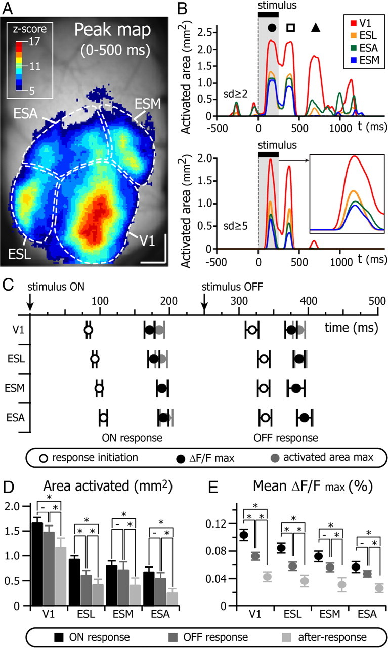
Spatiotemporal sequence of activation in the striate and extrastriate cortices. A, Peak map of the VSD response to a bright square flashed for 250 ms (averaged response of 50 trials) for an example experiment. V1: primary visual cortex; ESL: lateral extrastriate cortex; ESM: medial extrastriate cortex; ESA: anterior part of the extrastriate cortex. Boundaries between the different functional territories are defined on the basis of the least activated pixels located between two regions. B, Variation in time of the activated area (in mm²) in the four functional regions of the visual cortex (color code in inset) delimited in A. Pixels are activated when their ΔF/F value is >2 and 5 baseline SD (top and bottom graph, respectively). Note the ON response (circle), OFF response (square), and after-response (triangle) pattern. Inset, Enlargement of the time course of the ON response. C, Temporal sequence of activation in the primary and high-order visual cortices (average of 21 mice). Response initiation: time at which the ΔF/F crosses the threshold of 2 baseline SD (white dots). ΔF/F_max: time at which the ΔF/F reaches its maximum (black dots). Activated area max: time at which the activated area curve (as shown in B) reaches its maximum (gray dots). D, Maximal area activated during the ON, OFF, and after-responses in the four different functional regions of the visual cortex (21 mice). E, Maximal ΔF/F during the ON, OFF, and late response (21 mice). ⁻p > 0.05; *p < 0.05. Z-score from 5 to 17 correspond to 0.06–0.16% of ΔF/F.

To quantify the visual responses across the population, we obtained a measure of the activity per functional area by calculating the mean activity of all pixels within each area as a function of time. We measured response latency as the time at which the average response crossed a threshold of 2 SD of the background noise calculated from a 500 ms baseline for each animal (0.0168 ± 0.0105%, mean ± SD, n = 21 mice). In the population, as with the example shown above, V1 was activated first with a latency of the ON response of 83.7 ± 12.5 ms (n = 21 mice, paired t test: ESL, p < 0.0001; ESA, p = 0.0002; and ESM, p < 0.0001), followed by ESL (92.4 ± 12.3 ms; n = 21 mice, paired t test: ESA, p = 0.01 and ESM, p = 0.04, then ESA and ESM started depolarizing at approximately the same time (105.3 ± 25.5 ms; n = 21 mice and 99.4 ± 18.9 ms; n = 21 mice, respectively, paired t test: p = 0.16) (Fig. 3C). Despite the differences in onset latency, ΔF/F signal of the ON response reached a peak almost simultaneously in all four functional regions of the visual cortex (V1: 171.8 ± 32.9 ms; ESL: 177.9 ± 36.7 ms; ESM: 189.9 ± 37.6 ms; ESA: 191.2 ± 33.8 ms; n = 21 mice; all t test p > 0.05) (Fig. 3C). However, the value of ΔF/F of V1 (0.104 ± 0.037%; n = 21 mice) was largest (paired t test: p = 0.007, p < 0.0001, and p < 0.0001 for ESL, ESA, and ESM, respectively) (Fig. 3D). ESL maximal ΔF/F (0.084 ± 0.033%; n = 21 mice) was also larger than the one of ESA (0.057 ± 0.037%; n = 21 mice) and ESM (0.072 ± 0.035%; n = 21 mice; paired t test: p < 0.0001 and p = 0.009, respectively). The response in ESA was the weakest (paired t test: p = 0.009) (Fig. 3D). The time at which the area activated by the ON response was maximal was the same in all territories (V1: 185.3 ± 35.6 ms; ESL: 188.4 ± 37.9 ms; ESA: 196.0 ± 42.4 ms; ESM: 189.5 ± 33.8 ms, n = 21 mice; paired t test: p > 0.05 for all comparisons) (Fig. 3C). Using the activated area curve calculated for each region (with a 2 SD threshold; Fig. 3D), we measured maximal activated areas of 1.64 ± 0.50 mm² in V1, 0.92 ± 0.34 mm² in ESL, 0.67 ± 0.46 mm² in ESA, and 0.80 ± 0.46 mm² in ESM.

In 33% of experiments (7 of 21), the ON response was followed by a steady depolarization and no OFF or after-response could be seen. In the remaining animals (14 of 21) there was a clear OFF response between 60 and 80 ms after stimulus offset (V1: 68.9 ± 35.8 ms; ESL: 85.5 ± 33.1 ms; ESA: 87.7 ± 33.1 ms; ESM: 85.3 ± 32.4 ms; n = 14 mice), and the maximum value of ΔF/F of the OFF response was reached at approximately the same time in all visual areas (V1: 124.7 ± 33.1 ms; ESL: 136.3 ± 30.8 ms; ESA: 143.6 ± 39.2 ms; ESM: 132 ± 45.5 ms; n = 14 mice, all t test p > 0.15). The activated area was also maximal at the same time (Fig. 3C, gray dots). The OFF response compared with the ON response was significantly less intense in V1 and ESL (Fig. 3D). The maximal area activated was a little bit smaller in all regions during the OFF response; however, this difference was only significant for ESL (Fig. 3D).

In 86% of the cases with an OFF response (12 of 14 mice), a nonspecific after-response followed the activity evoked by the disappearance of the square. Similar late activity following OFF responses has been also described in 72% of the neurons of the macaque primary visual cortex (McLelland et al., 2010). This nonspecific after-response was mainly restricted to V1 (Figs. 2A,C, 3B,D) as the amplitude of the after-response in V1 was the only one greater than the amplitude of the noise (paired t test with SD of the baseline; 0.017 ± 0.010%, n = 21, p = 0.008, other comparison p > 0.05) (Fig. 3D). This after-response reached a peak of ΔF/F (0.042 ± 0.024%, n = 12 mice) 406.3 ± 79.9 ms after the stimulus offset and spread on a surface of 1.16 ± 0.65 mm² (n = 12 mice; Figs. 3D, 2A).

Retinotopic organization

After showing the existence of functional regions activated in parallel by a simple visual stimulus, we investigated how this functional organization corresponds to the known retinotopic organization of the visual cortex. We used different strategies to evidence the retinotopic organization of visual cortex in our experiments and compare our results with published electrophysiological and anatomical data (Wagor et al., 1980; Wang and Burkhalter, 2007). We first used flashed squares of 9 × 9° at 2–5 different locations of the visual field (Fig. 4A; n = 3 mice) and compared the position of the cortical response in V1 (Fig. 4B). During the first 100 ms after the onset of the stimulus the location of cortical responses was distinct and corresponded to the known retinotopic organization of V1 (Wagor et al., 1980; Schuett et al., 2002; Kalatsky and Stryker, 2003; Tohmi et al., 2006; Wang and Burkhalter, 2007) (Fig. 4B, left). Between 100 and 150 ms after stimulus onset the activated areas overlapped but their centers remained the same (Fig. 4B, right). This spread of depolarization around a response center (already shown Fig. 2A,D) suggests that the corticocortical recurrent activity activated by visual stimuli extends beyond the initial retinotopic position. This phenomenon had already been described in the cat V1 (Jancke et al., 2004; Sharon et al., 2007) and rat and mouse barrel cortex (Petersen et al., 2003; Civillico and Contreras, 2006; Ferezou et al., 2006) and here we generalized it to the mouse.

Figure 4.

Evoked responses in V1 are not restricted to the retinotopy of the initial response. A, Peak maps of the response of V1 to the presentation at four different location of the screen of a 9 × 9° bright square (luminance: 153 Cd/m²) on a gray background (luminance: 83 Cd/m²) (n = 10 trials for each location). For each position, a peak map was computed between 50 and 100 ms (top), and 100 and 150 ms (bottom). B, Superimposition of the peak maps shown in A. Each peak map has been assigned a color as indicated in the inset above. Colors have been set in transparency so pixels activated by more than one position appear in a shade resulting from the mix of primary colors. Threshold of 4 SD correspond to 0.06% of ΔF/F.

To more efficiently generate a complete mapping of visual space, we used oriented bars (vertical or horizontal, size: 9° × 75° and 9 × 56° degrees, respectively, luminance: 153 Cd/m²) drifting across the screen within 2 s in four different directions (left ↔ right and top ↔ bottom, velocity: 37.5 and 28°/s, respectively) (Fig. 5A, top row). When the drifting bar entered the visual field, it activated the corresponding edge of primary and extrastriate cortex. In Figure 5A, the bar (top row) is represented at its position 80 ms before the first detected response since that was the mean latency of our optical responses (see above). Thus, when the bar was on the top of the screen it activated the posterior part of V1 (Fig. 5A, first column), whereas when the bar was on the bottom of the screen it activated the anterior part of V1 (Fig. 5A, second column). The presentation of drifting vertical bars also allowed determining the azimuthal boundaries of the visual field representation. The presence of the bar on the left of the screen activated the lateral part of the contralateral V1 (Fig. 5A, third column), whereas a bar located on the right activated the medial part of the contralateral V1 (Fig. 5A, fifth column). All previous instances also activated the extrastriate cortex.

Figure 5.

Cortical activity evoked by a bar traveling across the visual field (single trials). A, Sequence of five consecutive single trials. Four trials consist in a bright bar (153 Cd/m²; 75 × 9° [horizontal bars] or 9 × 56° [vertical bars]), crossing a gray screen in 2 s (83 Cd/m²) in four different directions (top to bottom, bottom to top, left to right, and right to left). For one trial no stimulus is shown (No stim). Bottom row, Single frame acquired when the bar is located at the position indicated in A. For the No Stim trial, the snapshot has been replaced by the image of the surface of the occipital cortex and the location of the 5 × 5 pixels areas from which traces are presented in B. The four functional regions are delimited by dotted lines. Scale bars: 0.5 mm. B, Simultaneous recording of the ΔF/F (8 bottom traces) and the motor cortex EEG (top traces) for the five consecutive single trials (from left to right). Vertical arrows delimit the time period during which bars cross the screen. Inset, Enlargement and superimposition of the variation of the ΔF/F indicated by dotted boxes. Note that the sequence of activation is inverted when the bar is moving in the opposite direction. Z-score from 4 to 10 correspond to 0.18 to 0.45% of ΔF/F.

While the bar progressed across the visual field the fluorescence signal moved steadily across the cortex and extinguished at the opposite side from where it started. This sequential activation of the cortex was clear in the variation of the ΔF/F taken from ROIs at different locations of V1 (Fig. 5B, ROIs indicated by the squares in fourth column in A). A horizontal bar traveling from bottom to top activated first the anterior part of V1 then the posterior part, whereas the bar with the same orientation but traveling in the opposite direction activated V1 in the reverse sequence (Fig. 5B, first and second columns, respectively; see superimposed traces below). The same was true for left and right movement (Fig. 5B, compare third and fifth columns).

We averaged the responses to the horizontal and vertical bars drifting at a constant velocity for 2 s (n = 14 mice; 10–50 presentations for each direction). Each recording lasted 4 s in which we presented an isoluminant gray screen for 1 s, followed by a bright bar drifting across the screen for 2 s, followed by the presentation of an isoluminant gray screen for 1 s. Using the time difference between the appearance and the disappearance of the response in V1, we could estimate the size of the visual field mapped in the contralateral cortex to be 38.7 ± 6.4° (elevation, n = 14 mice) by 53.6 ± 7.1° (azimuth; n = 14 mice) (Fig. 6A). This size of the represented visual field corresponds to the one described by Kalatsky and Stryker (2003) using intrinsic imaging. To create a retinotopic map from these data it is necessary to determine for each pixel the position of the bar that elicits the maximal response. This is not possible directly due to fluorescence noise that prevents determining a reliable maximum for the evoked activity in each pixel (Fig. 6B, top left). Instead, we generated an arbitrary temporal reference in the shape of a Gaussian function centered at 2000 ms with respect to the beginning of the trial and with a SD of 500 ms (Fig. 6B, top right trace). This curve well describes the time course of activation at the center of V1 (Fig. 6B, top left), the rise and decay of the ΔF/F in the extrastriate areas. We then calculated the cross-correlation function between the activation profile of each pixel and this theoretical reference Gaussian and used the peak offset from zero (corresponding to the appearance of the drifting bar at one extremity of the screen) as the time of activation for that pixel. To avoid measuring the time peak of pixel having a low correlation with the Gaussian, we displayed only pixels with a peak of correlation above a threshold (mean cross-correlation threshold value = 0.3 ± 0.1; n = 14 mice). The offset from zero ranged from 0.3 to 1.8 s (n = 14 mice). The offset of the cross-correlograms was represented as pseudocolor (32 equally spaced colors from red to blue or short to long) for the horizontal (Fig. 6B) and the vertical (Fig. 6C) bar to generate retinotopic maps of the visual cortex (Fig. 6B, bottom left). To assess the reliability of this method, we compared the retinotopic maps provided by the datasets obtained in the same animal for bars of the same orientation traveling in the opposite directions (Fig. 6C,D). In all of our experiments (n = 14 mice), we found a good correspondence between the map obtained with the horizontal bar going from bottom to top or from top to bottom (Fig. 6C) and the vertical bar going from right to left or left to right (Fig. 6D) in V1 and ESL. In V1, the top of the visual field was represented in the caudal part and the bottom of the visual field in the rostral part, at the border with ESA and ESM. The most medial portion of the contralateral visual field was represented on the lateral part of V1 and the lateral periphery of the visual field on the medial part of V1. This organization of V1 corresponds to the one already described using electrophysiological and anatomical techniques (Wagor et al., 1980; Wang and Burkhalter, 2007). ESL presents several retinotopical maps. In all of our experiments, we could distinguish two main maps corresponding to the anterolateral (AL) area and the lateromedial (LM) area (Wang and Burkhalter, 2007) of ESL also obvious in some experiments with the flashed square (Fig. 2B,D). Two other areas in ESL (laterointermediate area and posterior area) described anatomically (Wang and Burkhalter, 2007) could be found in some animals (Fig. 6C,D). In 11 animals (78.6%), ESM was obviously subdivided in two retinotopic maps corresponding to the anteromedial (AM) area and the posteromedial (PM) area of the extrastriate cortex (Wang and Burkhalter, 2007; Fig. 3A). In none of the animals could we find a clear and robust retinotopic organization of ESA (Fig. 6C,D) certainly due to the fact that projections from V1 to this region are sparse (Wang and Burkhalter, 2007) leading to a signal too weak for the sensitivity of our experimental setup.

Figure 6.

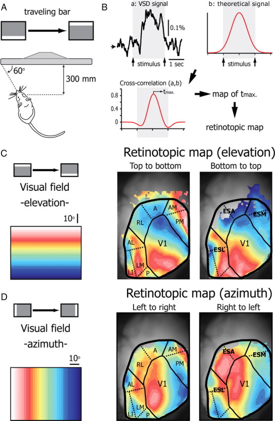
Retinotopy of the primary visual cortex and the extrastriate areas determined with VSD imaging. A, Schematic representation of the experimental setup. Bars (4 different directions) traveling across the screen in 2 s were presented to the eye contralateral to the imaged cortex. B, Construction of the retinotopic maps. For each direction the response of pixels is averaged over 50 trials (a: VSD signal). For each pixel, the time of activation is defined as the time at which the cross-correlogram (cross-correlation a,b) between the VSD signal of the pixel (a: VSD signal) and a Gaussian curve reference (b: reference) reaches its maximum (t_max). Color maps (presented in C and D) are created by assigning to each pixel its t_max value. C, Retinotopic maps of the elevation calculated using the VSD signal evoked by a horizontal bar crossing the screen from top to bottom (left map) or from bottom to top (right map). Color code of the elevation is indicated on the left. D, Retinotopic map of the azimuth calculated using the VSD signal evoked by a vertical bar crossing the screen from left to right (left map) or from right to left (right map). The boundaries of V1, ESL, ESA, and ESM are delimited by solid lines. Dotted lines highlight distinct retinotopically organized extrastriate areas described anatomically by Wang and Burkhalter (2007). A, anterior area; AL, anterolateral area; AM, anteromedial area; LI, laterointermediate area; LM, lateromedial area; P, posterior area; PM, posteromedial area; RL, rostrolateral area.

Propagating and standing waves

Once we studied the retinotopic organization of the four regions of the visual cortex, we investigated the dynamics of the individual responses. VSD imaging studies conducted in the visual cortex of the deeply anesthetized rat suggested the existence of propagating waves beyond (Xu et al., 2007) and within (Han et al., 2008) V1 during synchronized EEG states. We wanted to test the propensity of these propagating activities that occur in mice during neuroleptanalgesia when the EEG is in a desynchronized state and the cortical neurons are depolarized (Constantinople and Bruno, 2011). The analysis of propagation has to be done at the single trial level since averaging of responses propagating in different directions renders stationary waves. We studied 567 single trial responses in 21 mice to a flashed bright square (250 ms, 153 Cd/m²) on a gray background (83 Cd/m²). The probability to detect a response in single trials (using 2 SD above baseline noise as criterion) was 0.79 ± 0.10 in V1, 0.70 ± 0.20 in ESL, 0.3 ± 0.3 in ESA, and 0.38 ± 0.23 in ESM (n = 21 mice). Single trial responses in V1 generated a wave that propagated beyond the boundaries of V1 in 23 ± 12% of trials (mean of means of 21 mice), or a wave propagating locally within V1, characterized by the displacement of the center of activation within V1, in 16 ± 9% of trials (mean of means of 21 mice). In the remaining trials (61%), the responses did not propagate but remained anchored to their centers. Thus, rather than traveling as a wave, we found that even at the single trial level the response evoked by a discrete visual stimulus arises and remains centered on its cortical response field rather than travel.

Local recurrent activity is a function of the stimulus intensity

Next we measured the effect of stimulus luminance on response parameters. In six mice we measured the responses to flashed squares (250 ms, 18 × 18°; Fig. 7A) of 15 different luminance levels (7 bright, 7 dark, 1 mean gray background; Fig. 7B, luminance values indicated on top of frames in C) on an even gray background (83 Cd/m²). From the averaged ON responses (30–50 trials) we quantified response magnitude as (1) the maximal area activated and (2) the average value of the ΔF/F within the four cortical visual regions. In Figure 7C, we show for the same animal the movie frames at which the maximal activated area was reached for the 15 different luminance levels (time from stimulus onset is indicated on the top right corner). This figure shows that the maximum areas activated in response to the four higher luminance levels were much larger for bright than for dark stimuli.

Figure 7.

Properties of the evoked response as a function of the stimulus intensity. A, Stimulus sequence, A bright square of 18 × 18° is flashed for 250 ms on a gray background (83 Cd/m²). B, The contrast between the luminance of the square and the background could take 15 values ranging from −83 Cd/m² to +70 Cd/m². C, Single frames (average of 50 trials) corresponding to the maximal area activated in V1 during the ON response. ΔF/F is expressed as z-score (scale on the bottom right). For each contrast (indicated above each frame) this maximal activation occurred after the delay indicated on the top right corner of the image. D, Plot of the maximal surface activated (threshold 2 baseline SD) during the ON response for V1, ESL, ESM, and ESA (n = 6). E, Maximum values of the ΔF/F in the four functional regions of the visual cortex (n = 6). F, Delay between the stimulus onset and the response initiation (black trace), the ΔF/F_max (light gray), and the maximal activated area (activated area max., dark gray) in the V1 as a function of the stimulus contrast.

As shown in Figure 7C, the population means of the maximum area activated for the highest stimulus luminance also showed a strong asymmetry between bright and dark stimuli, and the difference was significant in V1 and ESL (Fig. 7D; Table 1). The maximum activated area showed some degree of dependence on luminance only for bright stimuli and mainly in V1 (Fig. 7D; constraint a = 0, i.e., start at the origin; Table 2). Similarly to the area of activation, the response magnitude to the highest luminance stimulus, given by the values of the average ΔF/F over each region, displayed a tendency for being higher for bright than dark stimuli (Fig. 7E; Table 3). The slope of the maximum ΔF/F as a function of luminance obtained from linear fits to the averaged data were very shallow and only clearly dependent on luminance in V1 and ESL for bright stimuli (Fig. 7E; constraint a = 0, i.e., start at the origin; Table 4).

Table 1.

Maximum area activated for the highest dark and bright luminance in the four functional regions of the visual cortex

Amax (n = 6 mice)	Bright	Dark	Paired t test
V1	1.68 ± 0.27 mm2	0.18 ± 0.07 mm2	p = 0.001
ESL	0.86 ± 0.17 mm2	0.28 ± 0.08 mm2	p = 0.012
ESA	0.64 ± 0.26 mm2	0.17 ± 0.10 mm2	p = 0.184
ESM	0.61 ± 0.30 mm2	0.015 ± 0.013 mm2	p = 0.095

Averaged value of the maximum area activated (A_max) for the highest dark (−83 Cd/m²) and bright (+70 Cd/m²) differential of luminance of the square with the isoluminant gray screen and the probability of these value to be different estimated with a paired t test (n = 6). ESL, lateral part of the extrastriate cortex; ESA, anterior part of the extrastriate cortex; ESM, medial part of the extrastriate cortex.

Table 2.

Dependence of the maximum activated area on luminance in the four functional regions of the visual cortex

Amax slope (n = 6 mice)	Bright (mm2/(Cd/m2))	Dark
V1	0.0239 (r = 0.959)	−0.0036 (r = −0.603)
ESL	0.0128 (r = 0.948)	−0.0039 (r = −0.827)
ESA	0.0082 (r = 0.867)	−0.0022 (r = −0.901)
ESM	0.0081 (r = 0.826)	−0.0005 (r = −0.376)

Slope of the linear fit of the curves A_max = f(variation of the luminance) presented in Figure 7D. The value of the Pearson correlation coefficient (r) is indicated in parentheses.

Table 3.

Response magnitude for the highest dark and bright luminance in the four functional regions of the visual cortex

DF/Fmax (n = 6 mice)	Bright	Dark	Paired t test p value
V1	0.094 ± 0.012%	0.045 ± 0.007%	p = 0.009
ESL	0.084 ± 0.009%	0.066 ± 0.005%	p = 0.067
ESA	0.060 ± 0.011%	0.056 ± 0.005%	p = 0.732
ESM	0.068 ± 0.013%	0.029 ± 0.010%	p = 0.018

Values of the average fractional fluorescence over each region for the highest dark (−83 Cd/m²) and bright (+70 Cd/m²) differential of luminance of the square with the isoluminant gray screen and the probability of these value to be different estimated with a paired t test (n = 6).

Table 4.

Dependence of the response magnitude on luminance in the four functional regions of the visual cortex

Amax slope (n = 6 mice)	Bright (%/(Cd/m2)	Dark
V1	0.00149 (r = 0.970)	−0.00064 (r = −0.955)
ESL	0.00141 (r = 0.969)	−0.00083 (r = −0.956)
ESA	0.00095 (r = 0.950)	−0.00062 (r = −0.917)
ESM	0.00096 (r = 0.966)	−0.00037 (r = −0.874)

Slope of the linear fit of the curves ΔF/F = f(variation of the luminance) presented in Figure 7E. The value of the Pearson correlation coefficient (r) is indicated in parentheses.

To quantify the time course of the responses as a function of luminance we measured the latencies to (1) response onset, (2) peak of ΔF/F, and (3) maximal area activated (Fig. 7F). The responses to bright stimuli showed a tendency to shorter onset latency (e.g., for the highest luminance R_Bright = 73 ± 8 ms and R_Dark = 84 ± 5 ms, p = 0.054). As well, higher luminance stimuli showed a tendency to shorten the latency of the visual response, but this tendency was more pronounced for bright than for dark stimuli (R_100%Bright = 73 ± 8 ms and R_50%Bright = 99 ± 13 ms, p = 0.005 // R_100%Dark = 84 ± 5 ms and R_50%Dark = 96 ± 6 ms, p = 0.043). There was no difference between bright and dark stimuli in the latency to peak of the ΔF/F, either at maximum or half-luminance (R_Bright = 149 ± 16 ms and R_Dark = 134 ± 7 ms, p = 0.349 // R_100%Bright = 149 ± 16 ms and R_50%Bright = 99 ± 13 ms, p = 0.108 // R_100%Dark = 134 ± 7 ms and R_50%Dark = 166 ± 24 ms, p = 0.226). Similarly, there were no differences in the latency to maximal area between highest luminance bright and dark stimuli or between half- and highest luminance (R_Bright = 143 ± 9 ms and R_Dark = 168 ± 20 ms, p = 0.498 // R_100%Bright = 143 ± 9 ms and R_50%Bright = 151 ± 11 ms, p = 0.240 // R_100%Dark = 168 ± 20 ms and R_50%Dark = 211 ± 29 ms, p = 0.312). Altogether these data suggest that the intensity of the stimulus modulates the strength of the feedforward thalamocortical input and the recurrent synaptic activity within the local networks of the striate and extrastriate cortices.

Discussion

We studied the properties of visually evoked activity in the mouse visual cortex during desynchronized EEG states using optical imaging with VSDs. Our main findings were as follows: (1) visual information is processed simultaneously in V1 and in three functional groups of high order visual cortices (ESL, ESA, and ESM) having distinct activation dynamics, (2) each functional group of extrastriate cortex is subdivided in areas organized retinotopically, (3) in each striate and extrastriate area the activity evoked by the stimulus is initiated retinotopically and subsequently spreads radially to adjacent nonretinospecific territories, and (4) this radial spread of activity is mostly a standing wave and the spatial extent of this activation depends on the intensity of the stimulus.

Parallel processing in the visual cortex

Our results show that during desynchronized EEG states, visual information is distributed in a retinotopically specific manner via long-range connections from V1 to higher order visual areas. These long-range connections can be mediated by corticothalamocortical connections or by direct corticocortical connections between the striate and extrastriate cortices (Wang and Burkhalter, 2007). In this study we show for the first time the sequence of activation evoked by a simple visual stimulus. The extrastriate cortex can be separated in three dynamically distinct functional groups containing several copies of the retinotopic map. The first extrastriate area activated (ESL) is located laterally to V1 and corresponds to the AL and the LM (Wang and Burkhalter, 2007). ESL has long been considered as a single entity and homologous of the primate V2 (Rosa and Krubitzer, 1999; Kalatsky and Stryker, 2003; Van den Bergh et al., 2010). However AL and LM have distinct cytoarchitectures and chemoarchitectures and project to different sets of cortical targets (Wang et al., 2011). In particular, the fact that AL projects preferentially to the medial entorhinal cortex whereas LM projections are stronger in the lateral entorhinal cortex suggests that AL and LM are the gateways of the dorsal and ventral streams, respectively (Wang et al., 2011). Two studies using calcium imaging recently confirmed that AL could belong to the dorsal stream as the neurons located there show high temporal frequency and direction selectivity (Andermann et al., 2011; Marshel et al., 2011). The role of ESA and ESM is much less understood. As these two regions are activated after ESL and are less sensitive to the stimulus contrast, it is likely that these regions represent a subsequent stage of visual information processing. This hypothesis is supported by anatomical evidence: V1, AL, and LM send massive projection toward the AM and the PM area (Wang and Burkhalter, 2007; Wang et al., 2011), two areas activated simultaneously in ESM. PM, whose neurons respond to low stimulus speed and relatively high spatial frequency, could be an area belonging to the ventral stream and specialized in object recognition (Andermann et al., 2011; Marshel et al., 2011). The two regions belonging to ESA, the rostrolateral area and anterior area, receive also projections from V1, AL, and LM (Wang and Burkhalter, 2007; Wang et al., 2011). The consecutive activation of V1, ESL, then ESA and ESM represent, to our knowledge, the first evidence of the existence in the mouse of parallel processing streams of visual information possibly distributing the analysis of specific parameters of the visual stimulus to distinct specialized areas.

Recurrent activity in the visual cortex

In addition to the parallel processing of visual information by different high-order visual cortices, we showed that within each region of the striate and extrastriate cortices, the surface activated by a stimulus (also called “cortical response field”; Sharon et al., 2007), extends over a large portion of the visual area, beyond the early retinotopic response, leading to a large amount of spatial overlap of visual responses. In the primary visual cortex of cats and primates, VSD imaging showed subthreshold synaptic potential spread far beyond the retinotopic area classically described as the region of action potential firing (Grinvald et al., 1994; Jancke et al., 2004; Benucci et al., 2007; Sharon et al., 2007; Chavane et al., 2011). Similar results were obtained using field potential measurements (Kitano et al., 1995; Nauhaus et al., 2009) or intracellular recordings (Bringuier et al., 1999). A radial spread of activity beyond the anatomical boundaries of the corresponding barrel has also been described during whisker stimulation in rodents (Petersen et al., 2003; Civillico and Contreras, 2006; Ferezou et al., 2006). Intracortical connections provided by horizontal projections of layer 2/3 neurons (Burkhalter, 1989) are likely to be responsible for this spread of the evoked activity (Contreras and Llinas, 2001; Sharon et al., 2007; Chavane et al., 2011). Lateral activity enhances the specificity and reliability of visual responses (Haider et al., 2010) and is thought to be the physiological mechanism underlying line motion illusion (Jancke et al., 2004).

Our study of the variation of the evoked response with stimulus intensity provides further insight on how this retinotopically nonspecific activity is recruited. We found that the response to an intense stimulus arises sooner and propagates further than that to a weak stimulus. The variation of the latency of the response with contrast is in line with measurements from single cells (Dean and Tolhurst, 1986; Carandini and Heeger, 1994; Albrecht, 1995). The spatiotemporal profile of depolarization at the center and the periphery of the response in V1, and the variation of response intensity with contrast reported here are similar to those described in cats (Jancke et al., 2004; Chavane et al., 2011) and in awake monkeys (Sit et al., 2009). This later study showed that the spatial profile of the peak response is independent of stimulus contrast. This may seem as a discrepancy with our claim that the maximal area activated with high contrast stimuli is larger than the one activated by low contrast. However, Sit et al. (2009) compared the absolute spatial profile of the response using normalized Gaussian fits of the response while we present the area whose pixel value crosses a given threshold of ΔF/F. When rescaled to the absolute value of the ΔF/F, their results are comparable to ours. Another study that appears to contradict our findings showed visually evoked responses that were spatially restricted even when the contrast of full-screen drifting gratings increased (Nauhaus et al., 2009). It is possible that full-screen stimuli of high contrast recruit massive local inhibition (Mateo et al., 2011), which then prevents the propagation of recurrent activity. Altogether our results on the contrast dependence of the lateral spread suggest that the intensity of the recruitment of polysynaptic pathways and recurrent connections within the visual cortex are dependent on the intensity of the visual stimulus.

One surprising finding of our study is the greater sensitivity of the visual cortex of the mouse to bright compared with dark stimuli. It is likely that this difference originates in the retina where the segregation of responses signaling light increments and decrements into parallel ON and OFF pathways is initiated (Hartline, 1938). This segregation begins at the first synapse of photoreceptors with bipolar cells (Werblin and Dowling, 1969). In macaques and cats, the OFF pathways dominate in the central retina (Ahmad et al., 2003), in the thalamus (Jin et al., 2008, 2011), and in V1 (Yeh et al., 2009; Xing et al., 2010), generating larger visual-evoked potentials than lights (Zemon et al., 1988). Surprisingly, our results suggest that in mice the ON pathway dominates visual responses instead.

Propagating waves during desynchronized EEG state

Our analysis of single trials shows that in 23% of cases visual stimuli triggered a wave of depolarization that center travels beyond the boundaries of V1. However, we did not find activities such as compression activity (Xu et al., 2007) and spiral waves (Huang et al., 2010), which were reported in rats anesthetized with 1.5–2% isoflurane, urethane, or pentobarbital. Spontaneous propagating waves are a well described phenomenon during highly synchronized EEG states associated with anesthesia (Contreras et al., 1996; Mohajerani et al., 2010) and slow-wave sleep (Massimini et al., 2004). The role and the cellular mechanisms of these large-scale propagating activities are still poorly understood. Under neuroleptanalgesia, an anesthesia that preserves quiet wakefulness EEG dynamics (Constantinople and Bruno, 2011), we found that ∼40% of the trials initiate waves traveling locally or beyond the boundaries of V1. It is possible that these activities occur during synchronous periods (Fig. 1B), which can trigger spontaneous propagating waves in mice during quiet wakefulness (Mohajerani et al., 2010).

References

- Ahmad KM, Klug K, Herr S, Sterling P, Schein S. Cell density ratios in a foveal patch in macaque retina. Vis Neurosci. 2003;20:189–209. doi: 10.1017/s0952523803202091. [DOI] [PubMed] [Google Scholar]
- Albrecht DG. Visual cortex neurons in monkey and cat: effect of contrast on the spatial and temporal phase transfer functions. Vis Neurosci. 1995;12:1191–1210. doi: 10.1017/s0952523800006817. [DOI] [PubMed] [Google Scholar]
- Allman JM, Kaas JH. A representation of the visual field in the caudal third of the middle tempral gyrus of the owl monkey (Aotus trivirgatus) Brain Res. 1971;31:85–105. doi: 10.1016/0006-8993(71)90635-4. [DOI] [PubMed] [Google Scholar]
- Alves HC, Valentim AM, Olsson IA, Antunes LM. Intraperitoneal anaesthesia with propofol, medetomidine and fentanyl in mice. Lab Anim. 2009;43:27–33. doi: 10.1258/la.2008.007036. [DOI] [PubMed] [Google Scholar]
- Andermann ML, Kerlin AM, Roumis DK, Glickfeld LL, Reid RC. Functional specialization of mouse higher visual cortical areas. Neuron. 2011;72:1025–1039. doi: 10.1016/j.neuron.2011.11.013. [DOI] [PMC free article] [PubMed] [Google Scholar]
- Ayzenshtat I, Meirovithz E, Edelman H, Werner-Reiss U, Bienenstock E, Abeles M, Slovin H. Precise spatiotemporal patterns among visual cortical areas and their relation to visual stimulus processing. J Neurosci. 2010;30:11232–11245. doi: 10.1523/JNEUROSCI.5177-09.2010. [DOI] [PMC free article] [PubMed] [Google Scholar]
- Benucci A, Frazor RA, Carandini M. Standing waves and traveling waves distinguish two circuits in visual cortex. Neuron. 2007;55:103–117. doi: 10.1016/j.neuron.2007.06.017. [DOI] [PMC free article] [PubMed] [Google Scholar]
- Bringuier V, Chavane F, Glaeser L, Frégnac Y. Horizontal propagation of visual activity in the synaptic integration field of area 17 neurons. Science. 1999;283:695–699. doi: 10.1126/science.283.5402.695. [DOI] [PubMed] [Google Scholar]
- Burkhalter A. Intrinsic connections of rat primary visual cortex: laminar organization of axonal projections. J Comp Neurol. 1989;279:171–186. doi: 10.1002/cne.902790202. [DOI] [PubMed] [Google Scholar]
- Carandini M, Heeger DJ. Summation and division by neurons in primate visual cortex. Science. 1994;264:1333–1336. doi: 10.1126/science.8191289. [DOI] [PubMed] [Google Scholar]
- Chavane F, Sharon D, Jancke D, Marre O, Frégnac Y, Grinvald A. Lateral Spread of Orientation Selectivity in V1 is Controlled by Intracortical Cooperativity. Front Syst Neurosci. 2011;5:4. doi: 10.3389/fnsys.2011.00004. [DOI] [PMC free article] [PubMed] [Google Scholar]
- Civillico EF, Contreras D. Integration of evoked responses in supragranular cortex studied with optical recordings in vivo. J Neurophysiol. 2006;96:336–351. doi: 10.1152/jn.00128.2006. [DOI] [PubMed] [Google Scholar]
- Constantinople CM, Bruno RM. Effects and mechanisms of wakefulness on local cortical networks. Neuron. 2011;69:1061–1068. doi: 10.1016/j.neuron.2011.02.040. [DOI] [PMC free article] [PubMed] [Google Scholar]
- Contreras D, Llinas R. Voltage-sensitive dye imaging of neocortical spatiotemporal dynamics to afferent activation frequency. J Neurosci. 2001;21:9403–9413. doi: 10.1523/JNEUROSCI.21-23-09403.2001. [DOI] [PMC free article] [PubMed] [Google Scholar]
- Contreras D, Destexhe A, Sejnowski TJ, Steriade M. Control of spatiotemporal coherence of a thalamic oscillation by corticothalamic feedback. Science. 1996;274:771–774. doi: 10.1126/science.274.5288.771. [DOI] [PubMed] [Google Scholar]
- Dean AF, Tolhurst DJ. Factors influencing the temporal phase of response to bar and grating stimuli for simple cells in the cat striate cortex. Exp Brain Res. 1986;62:143–151. doi: 10.1007/BF00237410. [DOI] [PubMed] [Google Scholar]
- Felleman DJ, Van Essen DC. Distributed hierarchical processing in the primate cerebral cortex. Cereb Cortex. 1991;1:1–47. doi: 10.1093/cercor/1.1.1-a. [DOI] [PubMed] [Google Scholar]
- Ferezou I, Bolea S, Petersen CC. Visualizing the cortical representation of whisker touch: voltage-sensitive dye imaging in freely moving mice. Neuron. 2006;50:617–629. doi: 10.1016/j.neuron.2006.03.043. [DOI] [PubMed] [Google Scholar]
- Ferezou I, Haiss F, Gentet LJ, Aronoff R, Weber B, Petersen CC. Spatiotemporal dynamics of cortical sensorimotor integration in behaving mice. Neuron. 2007;56:907–923. doi: 10.1016/j.neuron.2007.10.007. [DOI] [PubMed] [Google Scholar]
- Gao E, DeAngelis GC, Burkhalter A. Parallel input channels to mouse primary visual cortex. J Neurosci. 2010;30:5912–5926. doi: 10.1523/JNEUROSCI.6456-09.2010. [DOI] [PMC free article] [PubMed] [Google Scholar]
- Greenberg DS, Houweling AR, Kerr JN. Population imaging of ongoing neuronal activity in the visual cortex of awake rats. Nat Neurosci. 2008;11:749–751. doi: 10.1038/nn.2140. [DOI] [PubMed] [Google Scholar]
- Grinvald A, Lieke EE, Frostig RD, Hildesheim R. Cortical point-spread function and long-range lateral interactions revealed by real-time optical imaging of macaque monkey primary visual cortex. J Neurosci. 1994;14:2545–2568. doi: 10.1523/JNEUROSCI.14-05-02545.1994. [DOI] [PMC free article] [PubMed] [Google Scholar]
- Gross CG, Rocha-Miranda CE, Bender DB. Visual properties of neurons in inferotemporal cortex of the Macaque. J Neurophysiol. 1972;35:96–111. doi: 10.1152/jn.1972.35.1.96. [DOI] [PubMed] [Google Scholar]
- Haider B, Krause MR, Duque A, Yu Y, Touryan J, Mazer JA, McCormick DA. Synaptic and network mechanisms of sparse and reliable visual cortical activity during nonclassical receptive field stimulation. Neuron. 2010;65:107–121. doi: 10.1016/j.neuron.2009.12.005. [DOI] [PMC free article] [PubMed] [Google Scholar]
- Han F, Caporale N, Dan Y. Reverberation of recent visual experience in spontaneous cortical waves. Neuron. 2008;60:321–327. doi: 10.1016/j.neuron.2008.08.026. [DOI] [PMC free article] [PubMed] [Google Scholar]
- Hartline HK. The response of single optic nerve fibers of the vertebrate eye to illumination of the retina. Am J Physiol. 1938;121:400–415. [Google Scholar]
- Harvey MA, Valentiniene S, Roland PE. Cortica l membrane potential dynamics and laminar firing during object motion. Front Syst Neurosci. 2009;3:7. doi: 10.3389/neuro.06.007.2009. [DOI] [PMC free article] [PubMed] [Google Scholar]
- Huang X, Xu W, Liang J, Takagaki K, Gao X, Wu JY. Spiral wave dynamics in neocortex. Neuron. 2010;68:978–990. doi: 10.1016/j.neuron.2010.11.007. [DOI] [PMC free article] [PubMed] [Google Scholar]
- Jancke D, Chavane F, Naaman S, Grinvald A. Imaging cortical correlates of illusion in early visual cortex. Nature. 2004;428:423–426. doi: 10.1038/nature02396. [DOI] [PubMed] [Google Scholar]
- Jin J, Wang Y, Swadlow HA, Alonso JM. Population receptive fields of ON and OFF thalamic inputs to an orientation column in visual cortex. Nat Neurosci. 2011;14:232–238. doi: 10.1038/nn.2729. [DOI] [PubMed] [Google Scholar]
- Jin JZ, Weng C, Yeh CI, Gordon JA, Ruthazer ES, Stryker MP, Swadlow HA, Alonso JM. On and off domains of geniculate afferents in cat primary visual cortex. Nat Neurosci. 2008;11:88–94. doi: 10.1038/nn2029. [DOI] [PMC free article] [PubMed] [Google Scholar]
- Kalatsky VA, Stryker MP. New paradigm for optical imaging: temporally encoded maps of intrinsic signal. Neuron. 2003;38:529–545. doi: 10.1016/s0896-6273(03)00286-1. [DOI] [PubMed] [Google Scholar]
- Kitano M, Kasamatsu T, Norcia AM, Sutter EE. Spatially distributed responses induced by contrast reversal in cat visual cortex. Exp Brain Res. 1995;104:297–309. doi: 10.1007/BF00242015. [DOI] [PubMed] [Google Scholar]
- Langlois M, Polack PO, Bernard H, David O, Charpier S, Depaulis A, Deransart C. Involvement of the thalamic parafascicular nucleus in mesial temporal lobe epilepsy. J Neurosci. 2010;30:16523–16535. doi: 10.1523/JNEUROSCI.1109-10.2010. [DOI] [PMC free article] [PubMed] [Google Scholar]
- Marshel JH, Garrett ME, Nauhaus I, Callaway EM. Functional specialization of seven mouse visual cortical areas. Neuron. 2011;72:1040–1054. doi: 10.1016/j.neuron.2011.12.004. [DOI] [PMC free article] [PubMed] [Google Scholar]
- Massimini M, Huber R, Ferrarelli F, Hill S, Tononi G. The sleep slow oscillation as a traveling wave. J Neurosci. 2004;24:6862–6870. doi: 10.1523/JNEUROSCI.1318-04.2004. [DOI] [PMC free article] [PubMed] [Google Scholar]
- Mateo C, Avermann M, Gentet LJ, Zhang F, Deisseroth K, Petersen CC. In vivo optogenetic stimulation of neocortical excitatory neurons drives brain-state-dependent inhibition. Curr Biol. 2011;21:1593–1602. doi: 10.1016/j.cub.2011.08.028. [DOI] [PubMed] [Google Scholar]
- McLelland D, Baker PM, Ahmed B, Bair W. Neuronal responses during and after the presentation of static visual stimuli in macaque primary visual cortex. J Neurosci. 2010;30:12619–12631. doi: 10.1523/JNEUROSCI.0815-10.2010. [DOI] [PMC free article] [PubMed] [Google Scholar]
- Métin C, Godement P, Imbert M. The primary visual cortex in the mouse: receptive field properties and functional organization. Exp Brain Res. 1988;69:594–612. doi: 10.1007/BF00247312. [DOI] [PubMed] [Google Scholar]
- Mohajerani MH, McVea DA, Fingas M, Murphy TH. Mirrored bilateral slow-wave cortical activity within local circuits revealed by fast bihemispheric voltage-sensitive dye imaging in anesthetized and awake mice. J Neurosci. 2010;30:3745–3751. doi: 10.1523/JNEUROSCI.6437-09.2010. [DOI] [PMC free article] [PubMed] [Google Scholar]
- Nauhaus I, Busse L, Carandini M, Ringach DL. Stimulus contrast modulates functional connectivity in visual cortex. Nat Neurosci. 2009;12:70–76. doi: 10.1038/nn.2232. [DOI] [PMC free article] [PubMed] [Google Scholar]
- Niell CM, Stryker MP. Highly selective receptive fields in mouse visual cortex. J Neurosci. 2008;28:7520–7536. doi: 10.1523/JNEUROSCI.0623-08.2008. [DOI] [PMC free article] [PubMed] [Google Scholar]
- Petersen CC, Grinvald A, Sakmann B. Spatiotemporal dynamics of sensory responses in layer 2/3 of rat barrel cortex measured in vivo by voltage-sensitive dye imaging combined with whole-cell voltage recordings and neuron reconstructions. J Neurosci. 2003;23:1298–1309. doi: 10.1523/JNEUROSCI.23-04-01298.2003. [DOI] [PMC free article] [PubMed] [Google Scholar]
- Polack PO, Guillemain I, Hu E, Deransart C, Depaulis A, Charpier S. Deep layer somatosensory cortical neurons initiate spike-and-wave discharges in a genetic model of absence seizures. J Neurosci. 2007;27:6590–6599. doi: 10.1523/JNEUROSCI.0753-07.2007. [DOI] [PMC free article] [PubMed] [Google Scholar]
- Poulet JF, Petersen CC. Internal brain state regulates membrane potential synchrony in barrel cortex of behaving mice. Nature. 2008;454:881–885. doi: 10.1038/nature07150. [DOI] [PubMed] [Google Scholar]
- Roland PE, Hanazawa A, Undeman C, Eriksson D, Tompa T, Nakamura H, Valentiniene S, Ahmed B. Cortical feedback depolarization waves: a mechanism of top-down influence on early visual areas. Proc Natl Acad Sci U S A. 2006;103:12586–12591. doi: 10.1073/pnas.0604925103. [DOI] [PMC free article] [PubMed] [Google Scholar]
- Rosa MG, Krubitzer LA. The evolution of visual cortex: where is V2? Trends Neurosci. 1999;22:242–248. doi: 10.1016/s0166-2236(99)01398-3. [DOI] [PubMed] [Google Scholar]
- Rosanova M, Timofeev I. Neuronal mechanisms mediating the variability of somatosensory evoked potentials during sleep oscillations in cats. J Physiol. 2005;562:569–582. doi: 10.1113/jphysiol.2004.071381. [DOI] [PMC free article] [PubMed] [Google Scholar]
- Sachdev RN, Ebner FF, Wilson CJ. Effect of subthreshold up and down states on the whisker-evoked response in somatosensory cortex. J Neurophysiol. 2004;92:3511–3521. doi: 10.1152/jn.00347.2004. [DOI] [PubMed] [Google Scholar]
- Schuett S, Bonhoeffer T, Hübener M. Mapping retinotopic structure in mouse visual cortex with optical imaging. J Neurosci. 2002;22:6549–6559. doi: 10.1523/JNEUROSCI.22-15-06549.2002. [DOI] [PMC free article] [PubMed] [Google Scholar]
- Sharon D, Jancke D, Chavane F, Na'aman S, Grinvald A. Cortical response field dynamics in cat visual cortex. Cereb Cortex. 2007;17:2866–2877. doi: 10.1093/cercor/bhm019. [DOI] [PubMed] [Google Scholar]
- Simons DJ, Carvell GE, Hershey AE, Bryant DP. Responses of barrel cortex neurons in awake rats and effects of urethane anesthesia. Exp Brain Res. 1992;91:259–272. doi: 10.1007/BF00231659. [DOI] [PubMed] [Google Scholar]
- Sit YF, Chen Y, Geisler WS, Miikkulainen R, Seidemann E. Complex dynamics of V1 population responses explained by a simple gain-control model. Neuron. 2009;64:943–956. doi: 10.1016/j.neuron.2009.08.041. [DOI] [PMC free article] [PubMed] [Google Scholar]
- Steriade M, McCormick DA, Sejnowski TJ. Thalamocortical oscillations in the sleeping and aroused brain. Science. 1993;262:679–685. doi: 10.1126/science.8235588. [DOI] [PubMed] [Google Scholar]
- Timofeev I, Contreras D, Steriade M. Synaptic responsiveness of cortical and thalamic neurones during various phases of slow sleep oscillation in cat. J Physiol. 1996;494:265–278. doi: 10.1113/jphysiol.1996.sp021489. [DOI] [PMC free article] [PubMed] [Google Scholar]
- Tohmi M, Kitaura H, Komagata S, Kudoh M, Shibuki K. Enduring critical period plasticity visualized by transcranial flavoprotein imaging in mouse primary visual cortex. J Neurosci. 2006;26:11775–11785. doi: 10.1523/JNEUROSCI.1643-06.2006. [DOI] [PMC free article] [PubMed] [Google Scholar]
- Van den Bergh G, Zhang B, Arckens L, Chino YM. Receptive-field properties of V1 and V2 neurons in mice and macaque monkeys. J Comp Neurol. 2010;518:2051–2070. doi: 10.1002/cne.22321. [DOI] [PMC free article] [PubMed] [Google Scholar]
- Van Essen DC, Lewis JW, Drury HA, Hadjikhani N, Tootell RB, Bakircioglu M, Miller MI. Mapping visual cortex in monkeys and humans using surface-based atlases. Vision Res. 2001;41:1359–1378. doi: 10.1016/s0042-6989(01)00045-1. [DOI] [PubMed] [Google Scholar]
- Wagor E, Mangini NJ, Pearlman AL. Retinotopic organization of striate and extrastriate visual cortex in the mouse. J Comp Neurol. 1980;193:187–202. doi: 10.1002/cne.901930113. [DOI] [PubMed] [Google Scholar]
- Wang Q, Burkhalter A. Area map of mouse visual cortex. J Comp Neurol. 2007;502:339–357. doi: 10.1002/cne.21286. [DOI] [PubMed] [Google Scholar]
- Wang Q, Gao E, Burkhalter A. Gateways of ventral and dorsal streams in mouse visual cortex. J Neurosci. 2011;31:1905–1918. doi: 10.1523/JNEUROSCI.3488-10.2011. [DOI] [PMC free article] [PubMed] [Google Scholar]
- Werblin FS, Dowling JE. Organization of the retina of the mudpuppy, Necturus maculosus. II. Intracellular recording. J Neurophysiol. 1969;32:339–355. doi: 10.1152/jn.1969.32.3.339. [DOI] [PubMed] [Google Scholar]
- Xing D, Yeh CI, Shapley RM. Generation of black-dominant responses in V1 cortex. J Neurosci. 2010;30:13504–13512. doi: 10.1523/JNEUROSCI.2473-10.2010. [DOI] [PMC free article] [PubMed] [Google Scholar]
- Xu W, Huang X, Takagaki K, Wu JY. Compression and reflection of visually evoked cortical waves. Neuron. 2007;55:119–129. doi: 10.1016/j.neuron.2007.06.016. [DOI] [PMC free article] [PubMed] [Google Scholar]
- Yeh CI, Xing D, Shapley RM. “Black” responses dominate macaque primary visual cortex v1. J Neurosci. 2009;29:11753–11760. doi: 10.1523/JNEUROSCI.1991-09.2009. [DOI] [PMC free article] [PubMed] [Google Scholar]
- Zemon V, Gordon J, Welch J. Asymmetries in ON and OFF visual pathways of humans revealed using contrast-evoked cortical potentials. Vis Neurosci. 1988;1:145–150. doi: 10.1017/s0952523800001085. [DOI] [PubMed] [Google Scholar]