A quantitative analytic pipeline for evaluating neuronal activities by high throughput synaptic vesicle imaging

Abstract

Synaptic vesicle dynamics play an important role in the study of neuronal and synaptic activities of neurodegradation diseases ranging from the epidemic Alzheimer’s disease to the rare Rett syndrome. A high-throughput assay with a large population of neurons would be useful and efficient to characterize neuronal activity based on the dynamics of synaptic vesicles for the study of mechanisms or to discover drug candidates for neurodegenerative and neurodevelopmental disorders. However, the massive amounts of image data generated via high throughput screening require enormous manual processing time and effort, restricting the practical use of such an assay. This paper presents an automated analytic system to process and interpret the huge data set generated by such assays. Our system enables the automated detection, segmentation, quantification, and measurement of neuron activities based on the synaptic vesicle assay. To overcome challenges such as noisy background, inhomogeneity, and tiny object size, we first employ MSVST (Multi-Scale Variance Stabilizing Transform) to obtain a denoised and enhanced map of the original image data. Then, we propose an adaptive thresholding strategy to solve the inhomogeneity issue, based on the local information, and to accurately segment synaptic vesicles. We design algorithms to address the issue of tiny objects-of-interest overlapping. Several post-processing criteria are defined to filter false positives. A total of 152 features are extracted for each detected vesicle. A score is defined for each synaptic vesicle image to quantify the neuron activity. We also compare the unsupervised strategy with the supervised method. Our experiments on hippocampal neuron assays showed that the proposed system can automatically detect vesicles and quantify their dynamics for evaluating neuron activities. The availability of such an automated system will open opportunities for investigation of synaptic neuropathology and identification of candidate therapeutics for neurodegeneration.

Introduction

Recent studies on neurodegradation diseases, such as Alzheimer’s disease and Rett syndrome, include evidence provided by analysis of synaptic vesicle activities (Selkoe 2002; Zoghbi 2003; Cheung, Fu et al. 2006; Moretti, Levenson et al. 2006; Abramov, Dolev et al. 2009; Esposito, Fernandes et al. 2011). Synaptic vesicles store various neurotransmitters. They play essential roles in nerve impulse propagation by releasing neurotransmitters at synapses (Sudhof 2004). The quantity and intensity of vesicles are the most significant features for estimating the activity and function of live or cultured neurons in presynaptic imaging (Rizzoli and Betz 2004; Abramov, Dolev et al. 2009; Dreosti and Lagnado 2011). All presynaptic functions involve synaptic vesicles, either directly or indirectly (Sudhof 2004). Recently, optical microscopy imaging has been increasingly applied to study the synaptic activities in neural circuits (Dreosti and Lagnado 2011). Compared with traditional electrophysiology, these imaging methods (Dreosti and Lagnado 2011) allow identification of neuron locations and synaptic connections. In addition, with modern fluorescence microscopes the imaging process can now be fully automated so that assays can be carried out in a high-throughput manner (Hann and Oprea 2004). A cell population containing hundreds or even thousands of neurons can now be studied in its entirety, thus obtaining a much more comprehensive understanding of neural circuit function and more significant statistical power than the conventional means, in which only a few neuronal cells are investigated. Therefore, such high throughput synapse assays allow the research of the neuron activity of neurodegration diseases at a system level, with minimal human interference. However, these high-throughput neuronal activity studies are not being realized, largely due to the lack of informatics tools that can automatically interpret the massive amounts of synaptic imaging data.

A widely used method for imaging synaptic activities is via FM dyes (Cochilla, Angleson et al. 1999; Gaffield and Betz 2006). FM dyes are modified styryl dyes that selectively stain secretory membrane structures that are undergoing exocytosis and endocytosis; they have been used extensively to investigate synaptic vesicle recycling (Betz and Bewick 1992). By imaging the membrane staining and destaining process, we can study a set of presynaptic activities such as endocytosis, recycle time, vesicle-pool dynamics, and exocytosis (Cochilla, Angleson et al. 1999). In addition, this technique was recently used to detect early synaptic deficit in neurodegeneration conditions (Abramov, Dolev et al. 2009). The FM dye approach is an ideal candidate for high throughput synaptic studies, its advantages include wide application to multiple types of synaptic preparation and simple procedures. Moreover, for large scale data generated by high-throughput image screening or high content screening in drug discovery or other biological applications, automated analysis and quantization will be valuable (Wang, Zhou et al. 2009).

For an image-based method, information can be acquired by image quantification and statistical analysis. Intensity and morphological features, such as size, shape, and boundary, are key elements in measuring the outcome of a knocked-down gene, a treatment, or other experimental procedures (Yan, Zhou et al. 2008). The dynamic changes to synaptic vesicles before and after electric stimulation, which forces dye release, provide a convincing quantitative criterion for determining neuron activity. Therefore, a successful automated image analysis tool will enable large-scale screening for effectors on pre-synaptic activities and greatly accelerate neuronal mechanism studies and drug screening. In this paper, we propose an automated strategy to measure neuron activities based on the synaptic assay. It can be applied to any large-scale studies of neuron activity that use synaptic vesicles as measurement. Our automated pipeline, which, to our knowledge, is a brand new procedure for screening large scale neuronal synaptic vesicles, requires minimal human intervention and is capable of batch processing. With the proposed system, biologists can generate and process large amounts of imaging data with minimal manual analysis to study the pathology and treatment of neurodegenerative diseases.

There are several popular algorithms for spot or similarly-shaped object detection. In cell segmentation, the common strategy is the marker controlled watershed algorithm (Wang, Zhou et al. 2008; Zhou, Li et al. 2009). However, cell images are usually collected from multi-channels; for example, nuclei channel images can be used to detect and segment cytoplasm channel images (Wang, Zhou et al. 2008). However, for the synaptic assay, we only have single channel information and markers are not easy to obtain. In addition, in the cell image nuclei channel, objects do not locate inside any other structures and can be fairly easily detected using common contrast enhancement methods. On the other hand, synapses are projections onto dendrites; most pre-synaptic boutons are located on or near the dendrites and suffer from inhomogeneous fluorescence background due to non-specific FM dye binding to dendrites. Moreover, the size of synaptic vesicle boutons is much smaller than that of cells. Therefore, following the cell segmentation pipeline results in vesicle detection failures. Another strategy, the LBF level set algorithm (Li, Lebonvallet et al. 2007; Li, Kao et al. 2008; Fan, Zhou et al. 2009), usually applied to address inhomogeneous images, is a popular algorithm in medical image processing. Due to stain imperfection, the intensity of both vesicle boutons and their background structures vary by a fairly large range. The active contour-based method fails to accurately stop at boundaries of such spots and misses low-intensity weak spots as well. In addition, the standard thresholding-based methods (Gonzalez and Woods 2008) are also not able to solve the inhomogeneity issue. Another alternate, MSVST (Multi-Scale Variance Stabilizing Transform (Zhang, Fadili et al. 2008)), a denoising and enhancement method, is reported as a fast and effective solution for spot detection. However, this method itself cannot achieve high detection accuracy for our presynaptic imaging application because it does not deliver accurate segmentation. Because MSVST is effective to denoise and enhance the original image, we will include it in the pipeline as a module followed by several additional steps.

Fig. 1 shows example images of a dissociated hippocampal neuron stained with FM 1-43 dye to visualize the recycling synaptic boutons used in this work. Fig. 1b is a zoom-in look of the squared marked region in Fig. 1a. Fig. 1c was acquired with electric stimulation applied to destain. The active vesicles release the dye after the stimulation, and disappear in Fig. 1c. The inactive vesicles are usually dead or slowly releasing vesicles with low activity levels. These two categories are marked by differently directed arrows in Fig. 1b. From Fig. 1c, we notice that, in addition to inactive vesicles, there are also other neuronal structures, such as dendrites, and some undesired spots. Taking these image data as an example, we will discuss several challenges in the detection and quantification of vesicles.

Fig. 1.

An example image of the synaptic vesicle assay on a hippocampal neuron. (a) An example image of hippocampal neuron stained with FM 1-43 dye taken before stimulation; (b) A zoom-in version of the squared region in Fig. 1a. Arrows pointing southwest show the active synapses. Arrows pointing northeast illustrate the inactive synapses; (c) The same region of Fig. 1a after stimulation.

The first issue is image intensity inhomogeneity. Vesicle boutons across the image have different intensity distribution and background, as illustrated in Fig. 1. For example, some dark spots might be recognized as background if we set a global intensity threshold too high. On the other hand, there are weak vesicles that fall below the level of background intensity. These weak vesicle boutons, referred as spots with low intensity, are easily missed in conventional detection methods. The weak spots possess neither high intensity nor dramatic intensity gradients. In addition, in our application, another category of relatively weak vesicles is usually located within bright background regions. The intensity change between before- and after-destaining is not as obvious as other vesicles, thus we name it a relatively weak vesicle. As discussed above, the inhomogeneity issue should be addressed and local information would be helpful to accurately detect and segment vesicles for FM-143-based synaptic vesicle assay.

The second issue is the tiny size of the object of interest, ten pixels on average, which instantly fails many available algorithms designed for large spots. Because of this issue, the detection result is sensitive to noise, some of which is of similar size to the object. Noise is comprised of Gaussian white noise and Poisson noise introduced by physical mechanisms (Zhang, Fadili et al. 2008). Gaussian random noise can be easily removed by filtering. However, the Poisson noise is introduced during the imaging process; it is a result of the random nature of photon emission and thus needs extra effort to eliminate. In the synaptic vesicle bouton data, the Poisson noise corrupts the edge as well as the texture of the object, which results in difficulties in detection and segmentation. Since the vesicle bouton size is much smaller than cells and although some cell image processing pipelines may look appropriate for this application, they fail in several steps. These include the methods (Jung, Kim et al. 2010) to resolve the overlapped objects and the center of the detection regions. In addition, these methods suffer unacceptable rates of both false positives and false negatives.

Another source of aberration is blurring and out-of-focus. The objects of interest in this study are spots, or tiny fluorescent puncta. These spots do not possess clear boundaries, and in turn, the intensity of objects gradually fades from the center to the periphery. The blurring is caused by the diffraction phenomenon and imperfection of the optical imaging system. Moreover, since cultured neurons do not grow on the same plane, some regions of interest may be out of focus. These intrinsic blurring and artificial blurring hinder accurate detection and segmentation of vesicle spots.

There are also some undesired structures in the image which prevent accurate detection of vesicles. These structures include inactive vesicles and vesicle-like structures introduced by imperfect staining. Furthermore, neuron dendrite membranes are stained by the FM dye due to the staining imperfection. These structures should be addressed in the prepossessing or post-processing procedures.

To summarize, accurate detection of neuron vesicles is impeded by difficulties in image inhomogeneity, object size, noise removal, and artifacts introduced by imperfections in imaging. To address these issues, we developed an automated pipeline for vesicle detection and quantification to characterize synaptic activities using vesicle dynamics. Our pipeline employs a Multi-Scale Variance Stabilizing Transform (MSVST) to alleviate the Poisson noise and enhance the signals. Local information is then employed to solve the inhomogeneity issue. A new iterated procedure employing object size and local intensity in an adaptive thresholding manner is proposed to detect vesicles with high intensity background as well as weak vesicles. In addition, we define criteria especially for this application to filter false positives with morphological features. We also design novel algorithms to separate the overlapped tiny objects such as vesicles. We define a score to measure neuron activity using the density and intensity dynamics of vesicle boutons. This unsupervised method provides accurate results with automated, fast, and batch processing capabilities. In addition, we compare this method with a supervised method based on the popular SVM (support vector machine (Cortes and Vapnik 1995)) using most common image features for spot objects and feature selection strategies (Yan, Zhou et al. 2008) and discuss the application of these two strategies.

The paper is organized as follows. The Materials and Methods section describes our data and the workflow of our pipeline in detail. Here, we explain acquisition of images, image denoising and enhancement, adaptive thresholding to segment vesicles, post processing, feature extraction, scoring, and the supervised detection method. The experimental results and validation by comparing automated results with manual results are presented in the Experimental Results section. Algorithmic related issues and scientific generalization are discussed in the Discussion section. We summarize our work in the Conclusions section.

Materials and Methods

Fig. 2 illustrates the pipeline of the whole procedure of processing the synapse assay data. In this section, we first introduce the cell culture and imaging protocols. Then we present steps of vesicle detection and segmentation in detail, which are represented by blue blocks in Fig. 2. Then we will introduce feature extraction and the definition of the neuron activity score. The outputs of the system provide a straightforward score of neuron activity and various categories of vesicle features. We also briefly describe the supervised detection method and related issues at the end of the section.

Fig. 2.

The automated pipeline of vesicle detection and analysis. The outputs of the pipeline are quantified vesicle features and a neuron activity score for each synaptic vesicle image.

Hippocampal cell culture

Mouse hippocampal CA3-CA1 neurons were prepared from embryonic day 16 (E16) C57BL/6 mice. Briefly, the hippocampal region was dissected and dissociated with 0.25% trypsin at 37°C for 20 minutes. The cells were triturated to single cells and plated on poly-L-lysine coated coverslips (#1.0, about 0.14mm thick) at a density of 200 cells/mm² in neural medium (neurobasal with B27 supplement and glutamax). Cells were used between DIV 14 and DIV 21.

FM 1-43 dye loading, destaining and data imaging

The resting buffer consisted of 25mM HEPES, 119mM NaCl, 2.5mM KCl, 2mM CaCl₂, 2mM MgCl₂, 30mM Glucose, 10μM 6-cyano-7-nitroquinoxaline-2,3-dione (CNQX), and 50μM D,L-2-amino-5-phosphonovaleric acid (D,L-AP5), pH 7.4. Buffer was balanced with sucrose to 315 mmol kg⁻¹osM⁻¹. Field stimulation was achieved through parallel platinum electrodes immersed in the perfusion chamber, delivering 70 V, 1 ms pulses at 10 Hz. Cells were washed with resting buffer twice before they were incubated with resting buffer containing 10 μM FM 1-43. To load FM dye, cells were stimulated with 900 action potentials (APs). They were then washed extensively with resting buffer for 10 minutes. To destain, cells were continuously stimulated and fluorescence images were recorded for 3 minutes at 5 second intervals.

In this study, we made use of the first image before destaining and the last image after destaining. For imaging, cells were viewed via a 60× 1.4 NA objective on an inverted microscope. The microscope was equipped with a stage environment control box and the temperature was maintained at 37°C. In this application, each data set contained two images, the first was scanned after staining and washing, and the other was taken using the same hardware settings after the electric stimulation, which excited the neuron to release stained dye. If the stimulation forced a complete dye release, indicating that the neuron and vesicles were active, few bright spots were observed in the second image. Therefore, the differences between before and after stimulation can be employed as a measurement of activity.

Image preprocessing

Image preprocessing procedures are employed to correct artifacts to help achieve optimal results. Due to non-specific staining, some neuron structures other than vesicle boutons are stained and these structures are illuminated in both before and after destaining images. In addition, although biologists endeavor to keep identical conditions before and after stimulation, there are still slight differences, such as changes in locations of the same neuron structure and intensity of non-vesicle structures. If there is need for registration, we apply the Iterative Closest Point (ICP) algorithm (Besl and McKay 1992) to align the two images. ICP finds the closest point on a geometric entity, which is the foreground object in an image, to a given point. The ICP algorithm converges monotonically to the nearest local minimum of a mean-square distance metric and the rate of convergence is fast (Besl and McKay 1992). For each data set, we manually select four reference points from the stained structures from the first time point image. Since no severe deformations are observed, we find it sufficient to consider only rigid transformation with the ICP algorithm. Note that the registration is an optional step in the pipeline, which can be enabled if necessary. After registration is the global background correction step. When the same neuron component has been aligned at the same or very close Euclidean location for two image slides, a consistent intensity range is desired. To do this, linear image enhancement is applied to the second image to establish consistence with the first. For an image batch, we employ an averaged range to adjust the background.

Given a data set of registered and background corrected images, we can simply subtract the second image from the first to obtain the difference image. In this image, the staining artifacts are mostly removed. These structures include both inactive vesicles and non-vesicle structures. The following procedures, including MSVST enhancement and adaptive thresholding, will be performed on the difference image of each image set.

Image segmentation

One of the most challenging issues is overcoming image inhomogeneity to identify both weak vesicles and vesicles with high intensity. To address this issue, we implement the MSVST method to perform approximate gaussianization and stabilize the variance of a sequence of independent Poisson random variables filtered using a low-pass linear filter. This wavelet-based algorithm is fast and effectively controls the false discovery rate (FDR) (Zhang, Fadili et al. 2008). This transform will provide an enhanced and denoised map of the difference image. Then we propose an adaptive thresholding-based iteration to directly address the inhomogeneity issue. The adaptive thresholding takes affect only on a limited number of vesicle regions and considers only local information. Thus, it is able to identify vesicles located in both bright and dark background regions. In addition, the proposed adaptive thresholding strategy addresses the size issue by varying the region size threshold to accurately acquire object boundaries. The parameters are loosely set to allow as small a number of false negatives as possible. The reason is that the loose thresholding will introduce some false positives; however, false positives can be eliminated in post processing but false negatives are very complicated to retrieve. To reduce the number of false positives, filters are defined to remove the fake vesicles including isolated spots, non-vesicle structures, and weak-vesicle-like structures.

1. MSVST

We first briefly explain the MSVST method as an enhancement and denoising procedure. Assume [Y_n] is a sequence of output RVs (random variable) of a finite impulse response (FIR) filter h, and [X_n] is independent RVs; equation (1) stands and the goal is to stabilize the variance of Y_n. In this case, the filter h functions as an averaging filter to increase the signal-to-noise ratio at the output.

$$y_n=\sum _{i}h(i)x_{n-i}$$ (1)

Any form of transformations would not change the property of the variance of [Y_n]. The general form of VST (variance stabilization transform) is given as: $T(Y)=b\sqrt{Y+c}$. We follow the definitions of b and c described by Zhang, Fadili et al. 2008.

After the stabilization procedure, UWT (undecimated wavelet transform) is applied to enhance the signal, which is intensity in this case. A filter bank (h, g) is employed by UWT, W ={w₁, w₂, ···, w_J, a_J}, where w_j, 1≤ j ≤ J is the wavelet coefficient at scale j, and a_J is the coefficient at the coarsest resolution. The update from one resolution to the next can be represented as: a_j+1 = h[−k]^(j) * a_j and w_j+1 = g[−k]^(j) * a_j. The reconstruction is obtained as a_j = (h̃^(j) * a_j+1 + g̃^(j) * w_j+1). The filter bank (h, g, h̃, g̃) has to meet the reconstruction conditions defined by Zhang, Fadili et al. 2008.

With the given definition and formulation, UWT denoising with MSVST involves the following three major steps: 1) transformation: to obtain UWT coefficients with MSVST; 2) detection: to identify significant wavelet coefficients by hypothesis testing; and 3) estimation: to iteratively reconstruct the final estimate with the identified wavelet coefficients. The detailed iterative reconstruction procedure is described in Box 1 .

Box 1. Procedures of MSVST enhancement.

Given a filter bank (h, g = δ − h, h̃ = δ, g̃ = δ)

Initialization: a0 = x

for j = 0 to J −1

do

Calculate the approximation coefficients aj+1 = h[−k](j)*aj

Calculate wj+1 =Tj aj − Tj+1aj+1 with VST as $T_j{a}_j={\tau }_1^{-1/2}\sqrt{a_j+c_j}$

Where ${\tau }_k={\displaystyle \sum _i}{(h{[i]}^{(j)})}^k$ and c= (7τ2 / 8τ1)−(τ3 / τ2)

Employ hypothesis testing-based denoiser ψ to wj+1, ŵj+1 = ψwj+1

end for

Reconstruct a0 as ${\widehat{a}}_0=T_0^{-1}(T_J{a}_J+{\displaystyle \sum _{j=1}^J}{\widehat{w}}_j)$

The reconstructed map is an enhanced version of the original difference image. In this map, bright spots are more illuminated while weak spots and spots contaminated by noise have been strengthened. At the same time, the background noise has been reduced. Moreover, edges of vesicle boutons are more obvious than before the procedure. Fig. 3 illustrates the effect of MSVST. Fig. 3a shows the original image while Fig. 3b is the MSVST transformed version of the difference image. Fig. 3c illustrates Fig. 3b in a 3D view with the value of MSVST map on the z-axis.

Fig. 3.

An illustration of MSVST enhanced map. (a) Original Image; (b) MSVST enhanced map of the original image; (c) A 3D view of the enhanced map.

2. Adaptive thresholding

We propose an adaptive thresholding-based procedure on the MSVST enhanced map to address the inhomogeneity issue. The adaptive thresholding employs local information to identify vesicles of both high and low intensity. From Fig. 3, we notice that if a global thresholding method is applied to such an inhomogeneous image, neither large thresholds nor small ones will accurately segment objects of interest. A large threshold will cause a false negative problem, which is unacceptable in most applications. On the other hand, a small threshold cannot accurately segment vesicles because it might derive loose boundaries. In our data, some vesicles cluster in a group with relatively high intensity background, such as dendrites and axon terminals. We name these vesicle groups HIC (high intensity clusters). Therefore, local information should be considered to solve this typical inhomogeneity issue.

We apply an initial intensity threshold to the enhanced difference image generated by the previous step. This threshold is low enough to allow very limited number of false negatives. Then, on the binarized image, we apply an area threshold T_A to obtain regions larger than the given threshold for further processing. For each of these regions, we employ the MSVST-derived values and identify subregions with intensity larger than T_I. This T_I will shrink or split the original region by selecting points with intensity larger than the threshold. If the shrunk or split subregions have smaller areas than the updated area threshold T_A, we save these updated regions as segmented spots and do not process them any further. For subregions with a larger area than the updated T_A, they will go through the next iteration and are filtered by increased threshold T_I. This iterative procedure is presented in Box 2 and illustrated by Fig. 4.

Box 2. The process of adaptive thresholding to detect vesicles in HIC.

For regions with area A > TA

for j =1: MaxIter

find subregions with average intensity Ī >TI

for each subregion i

if subregion i with area Ai < TA

save subregion i

else subregion i enters into the next for loop

end if

end for

increase TI = TI + StepLength * j

decrease T = ae− j +TAL, where a>1 is a descending

coefficient and TAL is the lower bound of TA

end for

Fig. 4.

A simulated example of the proposed process of adaptive thresholding. (a) Unprocessed image regions; (b) The effect of increasing T_I. The region splits into two subregions; (c) The effect of another iteration of updatedT_A and increased T_I. One subregion is saved and the other enters into the next iteration (d).

The StepLength is the intensity increment. It linearly increases T_I during the iteration until reaching the intensity upper bound. On the other hand, the update of the area threshold is not linear. T_A approaches the lower bound in an inverse exponential manner. The lower bound of T_A is usually a large portion of the average size of the spots; in our application, it is set to a value smaller than 75% of average spot size derived by experiments.

As illustrated in Fig. 4, there is an HIC region and an isolated spot with low intensity and small area. The area of the isolated spot is smaller than the initial area threshold and is not processed by adaptive thresholding. Increased intensity threshold decreases the area of the HIC background, which is illustrated in Fig. 4b and 4c. Once spots fail to satisfy the area condition, which indicates identification of a vesicle from a relatively high intensity background, regions are saved as segmented spots. This process is illustrated in Fig. 4c and 4d.

3. Segment the overlapped vesicles

Overlapped objects are commonly found in cell assays. Accurate quantification and segmentation are required to measure neuron activity, and as such, the overlap issue must be addressed. There are two classes of algorithms solving this issue (Dejnozkova and Dokladal 2004; Zeng, Miao et al. 2009). The first one relies on curvature to detect crossing points (points C and D marked by yellow squares in Fig. 5), which typically have large curvature values on edges of overlapped spots. Once these points are detected, we can simply connect them with any line connection algorithm. However, in our case, the size of vesicles is too small (around 10 pixels) to accurately calculate the curvature of each point on the edge and to identify the crossing points. The second common strategy to solve this issue is based on the assumption that the shape of objects of interest can be approximated as round disks. The crossing points can then be identified using the radius and distance between centers of each object. However, in our application, the object size is too small to make any shape approximation or assumption. Therefore, this type of strategy also fails to accurately identify the crossing points. Here, we propose a method to solve this issue.

Fig. 5.

Segmentation of overlapped vesicles. Points A and B are central points for each overlapped spot and connected by a green line section. Points C and D are the crossing points and the black line section separates the two overlapped regions. Solid red line sections represent candidates to split the two regions while the red dashed-line sections illustrate the non-candidates which fail to cross the green line section.

Our proposed strategy starts with distance mapping. The binary image derived by adaptive thresholding is iteratively eroded by a one-pixel radius disk template until all pixels are zeros. The number of iterations at which a non-zero pixel is eliminated is the distance from the pixel to the edge. Edge points always have distance as one and center points (points A and B in Fig. 5) usually have the largest values in the distance map. With the distance mapping we first locate the central points of each spot region. Overlapped vesicle regions may not contain the local maxima with maximal distance. In this case, we follow a strategy similar to the watershed algorithm on the distance map, which is illustrated by Fig. 6. Since prior information about number of vesicles in an overlapped region is unknown, we first consider all the local maximum regions with the largest distance in the distance map as central regions for each candidate spot. Then we search along the downhill direction on the distance map until we identify another isolated local maximum. There are two typical cases illustrated in Fig. 6a and 6b. Fig. 6a demonstrates a case in which two overlapped regions have the same local maximum while Fig. 6b illustrates a case in which one region has a larger local maximum than the other. To differentiate the cases in Fig. 6b and 6c, we also check neighbors of local maxima in the distance map. If a local maximum spreads over pixels, it is not considered as a center point. Since the radius of a circular vesicle or the minor axis of an ellipsoid vesicle usually varies from 2–5, the repetition of the decreasing on the distance map are performed twice in our experiments. For local maximal regions containing more than one pixel, we employ central points of these regions.

Fig. 6.

An illustration of searching for the local maxima as the region central points.

On the distance map, points with a value of one are the edge points. An example of an overlapped region is provided in Fig. 7. We use a template to detect all possible crossing points. In the distance map, we first search for 2’s (green squares in Fig. 7b) with at least two 1’s (red squares in Fig. 7b) within its 4-connection neighborhood, with 90 degree difference. These 1’s are candidate crossing points. This procedure reduces the amount of candidate crossing points on the edge, which depends dramatically on the size and shape of the region. Then, for each pair of overlapped regions, centers are connected with a line section, illustrated by the green line in Fig. 5. After that, we employ an exhaustive search on the candidate crossing points and save pairs whose connecting line section crosses the line section linking the region centers. These sections are represented by the red solid lines in Fig. 5; the dashed lines represent non-candidate pairs whose linking line sections fail to intersect with the line connecting region centers (green line). Finally, we use the pair with the smallest distance (white squares in Fig. 7b) that crosses the center connection as the crossing point for the two overlapped regions. This line section is illustrated by the black line in Fig. 5. In our data, spot regions are usually lined up without dramatic direction change so that the center connection line section is always within the overlapped region, indicating that two crossing points are located on opposite sides of the line. This strategy can be easily generalized to cases in which multiple regions are overlapped in a line.

Fig. 7.

An example of identification of the crossing points of two overlapped regions. (a) An overlapped region example; (b) The distance map of Fig 7a. The candidates of crossing points are marked in red. The 2’s, according to which we select candidate crossing points, are marked green. Two white squares are the crossing points identified by our algorithm.

Post processing

The purpose of post processing is to remove false positives from vesicle detection results. These false positives are comprised of three major classes: 1) isolated spots, 2) non-vesicle structures introduced by staining imperfection, and 3) weak-vesicle-like spots. We define these classes and provide detailed description of removal of these false positives in the following.

a. Filtering isolated spots

Vesicles usually cluster in neuronal structures such as dendrites and axon terminals, and seldom isolate with each other within a neighborhood. Isolated spots with high intensity are probably introduced by staining imperfection. Therefore, these spots should be reconsidered. We can simply define a neighborhood size and count the total number of spots in the neighborhood. If no other spots exist, the neighborhood filtering removes the isolated spot.

b. Remove non-vesicle structures

The non-vesicle structures are generally introduced by staining imperfections. The majority of these structures are dead spots. These objects are high in intensity in both before and after destaining slides when compared with active vesicles. Although we notice that decreases in average intensity are larger in part of these objects than in active vesicles, the changing ratio is lower than that of active vesicles. The numerical changing ratio is defined as the ratio between intensity decrease of a certain region from before to after stimulation and the intensity before stimulation. Usually the ratio of an active vesicle is 1.5 times the ratio of dead vesicles. By discarding spots with slight changes in average intensity, we remove the majority of the second false positive group. Other types of non-vesicle structures are neuronal structures such as line-structure dendrites and other irregularly shaped structures. These objects can be easily eliminated by shape descriptors such as major axis length, convexity, etc.

c. Remove weak-vesicle-like structures

There is another class of false positives that are difficult to distinguish from true active vesicles. This category is similar to weak vesicles in relatively low intensity as well as trivial intensity change compared to active vesicles. Unlike weak vesicles, these regions seldom contain a subregion with higher intensity than the region’s average intensity. Therefore, to distinguish this category, we first shrink these weak-vesicle-like regions by erosion according to region areas with 1 or 2 pixel radius disks. Then we calculate the change ratio defined previously for the shrunken region. For active vesicles, the intensity in the center is higher; the intensity change ratio of the shrunken region between before and after stimulation is larger than that of an unmodified region. Based on this observation, we can discard regions with slight change to the ratio before and after shrinkage.

After the previous steps, including preprocessing, segmentation by adaptive thresholding on MSVST enhanced maps, and post processing to remove different categories of false positives, we now consider the result as our final detection result for vesicle image data.

Image quantification

Vesicle quantification extracts straightforward features of each vesicle bouton, including average intensity, area, perimeter, etc. On the other hand, there are certain image features that cannot be directly or spatially observed from an image. These features are extracted from the frequency transformed domain of the original image. In the following paragraphs, we will describe all extracted vesicle bouton features in both spatial and frequency domains.

The first feature category includes general information about vesicle shape, size, and intensity. This fourteen-feature set is comprised of maximal intensity, minimal intensity, average intensity, deviation of gray level, length of long axis, length of short axis, long axis/short axis, equivalent diameter, area, convex area, perimeter, eccentricity, orientation, and solidity.

The second feature category is Haralick co-occurrence texture feature (Wang, Zhou et al. 2009), which can be extracted from each of the gray level spatial-dependence matrices. There are totally 13 co-occurrence texture features defined. They are angular second moment, contrast, correlation, sum of squares, inverse difference moment, sum average, sum variance, sum entropy, entropy, difference variance, difference entropy, information measures of correlation, and maximal correlation coefficient.

Another feature category is the wavelet coefficients. Gabor wavelets (Feichtinger and Strohmer 1998) are directly connected with Gabor filters because they can be designed for a number of scales and orientations. The Gabor filters can be considered dilation and rotation-tunable line detectors. In addition, the texture information can be characterized by statistical information, such as mean and variance in a certain patch. Here we adopt the strategy described in detail by Manjunath and Ma, 1996. With five scales and seven orientations, we have a seventy-element feature vector for each input sample image: [μ₀₀σ₀₀μ₀₁σ₀₁ ···μ₄₆σ₄₆]. μ_ij is the mean and σ_ij is the standard deviation of the magnitude of the transform coefficients. i stands for the scale while j denotes the orientation.

The Zernike moment feature is a region-based shape descriptor which is used as a pattern feature in object recognition from shape. Zernike moments are derived from Zernike polynomials which present an orthogonal set (Boland, Markey et al. 1998). The orthogonality provides the uniqueness of features extracted by the polynomials. In addition, the moments defined in polar coordination are invariant with respect to their magnitude under rotation. In our implementation, we first locate the centroid of each image. Second, we define the maximum radius R as the farthest pixel from the centroid. The images are then normalized with the center of mass and the maximum radius R. The pixel (x,y) in the original image is represent by (ρ,θ), which is the projected image from a Cartesian to a polar coordinate. With the notation I (x, y) and I(ρ,θ) for intensities of original and projected images, respectively, the Zernike moment for each image is defined as:

$$Z_{nm}=\frac{n+1}{\pi }\sum _{x^{\prime }}\sum _{y^{\prime }}{V}_{nm}^{\ast }(\rho ,\theta )I(\rho ,\theta )$$

Where 0 ≤ m ≤ n, (n − m) is even, ρ≤1, $V_{nm}^{\ast }$ is the complex conjugate of a Zernike polynomial V_nm of degree n and angular dependence m, which is defined over the unit disk as V_nm (ρ, θ) = R_nm(ρ)exp(jmθ). R_nm (ρ) is the Zernike polynomials given by

$$R_{nm}(\rho )=\sum _{k=0}^{(n-m)/2}\frac{{(-1)}^k(n-k)!}{k!\left(\frac{n+m}{2}-k\right)!\left(\frac{n-m}{2}-k\right)!}{\rho }^{n-2k}$$

The magnitude of Z_nm will be used as features. We choose n =12 so that we obtain 49 moment features in total. Details are provided by Boland et al, 1998.

In addition to the features described above, we propose a feature category specially designed for this application. This category includes 1) the average intensity difference between before and after stimulation of a certain region, 2) the ratio of 1) to the average intensity before stimulation, 3) the average intensity difference between before and after stimulation of a shrunken region, 4) the ratio of 3) to the average intensity before stimulation of the shrunken region, 5) the average intensity difference between before and after stimulation of an expanded region (following a similar manner to the shrinkage, but expanding the region instead), and 6) the ratio of 5) to the average intensity before stimulation of the expanded region. These features illustrate the intensity changes between the same regions in original, shrunken, and expanded cases, which are the most important features experts use in manual labeling. In total, we extract 152 features for each vesicle.

Supervised method

We briefly describe the supervised method to detect and segment vesicle images. Although the proposed post-processing criteria in the unsupervised strategy remove most predictable false positives, it is interesting to question whether there are better fitted models using more features to identify vesicles. Support vector machine (SVM) is widely employed in a variety of classification problems in bioinformatics. Its advantages in avoiding overfitting, managing large scale feature space, and incorporating diverse kernel methods make it a suitable solution to solve classification problems. In our study, we apply LIBSVM software (Chang and Lin 2001) to classify vesicles and false positives. Five-fold cross validation (CV) is performed. In N-fold CV, the original data set is equally separated into N partitions. N-1 partitions are employed to train the classifier and one partition is left to test the performance of the classifier. This procedure is performed N times for all N partitions and the accuracy is an average of all N tests. The training data is obtained from manual vesicle labeling by our experts. Details of manual labeling will be provided in the next section.

In the situation in which the dimension of the feature space is very large, the classifier easily tends to be overfitted. Feature selection is a solution to solve this problem and desirably, it also can increase the accuracy of the classification result and better interpret the model. SVM-RFE (Support Vector Machine-Recursive Feature Elimination (Rakotomamonjy 2003)) is an efficient feature selection algorithm in a backward discarding manner. This procedure starts with all the features, then removes one feature each time, and all the features are ranked in the end. The ranking principle for each step is the coefficients of the weight vector w of a linear SVM. The procedure is illustrated in Fig. 8.

Fig. 8.

Procedure of SVM-RFE.

Scoring system

To summarize neuron activity based on the synaptic vesicle assay, one straightforward idea is to employ the summarization of vesicle features, such as intensity and area; alternately, averaged features can be employed. However, the average intensity and area, defined as the summation divided by the total number of vesicles, suffer when a large image contains a limited number of vesicles with average vesicle quality. More specifically, this measurement cannot differentiate a decent synaptic vesicle image (with a large number of vesicles) from an image indicating poor neuron activity (with a similar image size but only a limited number of vesicles). In this case, the strategy based on averaged information fails to provide the obvious differences between the decent and the poor cases.

$$\mathit{Score}=\frac{{\sum }_{i=1}^n({\overline{I}}_{\mathit{Before},i}-{\overline{I}}_{\mathit{After},i})}{\mathit{Area}}\times k$$ (2)

Since intensity change of the same spot-region between before and after destaining is the most significant feature that allows the measurement of neuron activity, we employ this descriptor as the major factor to score the neuron activity. The definition of the score is provided by equation (2). Ī_i is the average intensity of region i. Subscripts Before and After indicate the before and after stimulation cases. The Area is the size of the image data. k is a constant number, equal to 100 in our example to modify the score to around 1. Instead of averaging by the vesicle quantity, we utilize the size of the image to divide the total intensity of all detected vesicles. In this case, one image with a considerable number of vesicles has a higher score than the one with a limited number of vesicles of the same size. This is based on the assumption that neurons containing more vesicles releasing FM dye are more active or vigorous than those with a limited number of vesicles.

Since the fluorescence intensity of segmented puncta is the most important parameter for measuring the activity of pre-synaptic boutons, we propose a precise measurement strategy to accurately quantify this value. Subtraction images of the before and after destaining images allows global background correction; however, this method only measures the activity of fast recycling vesicles, which undergo exocytosis in the second round of stimulation (destaining). To measure the total vesicle activity, quantification of the image after FM dye uptake alone is necessary. However, this is hampered by the inhomogeneous background as the pre-synaptic boutons reside on or near dendrites to which FM dyes nonspecifically bind, illustrated in Figure 1. Global background correction is inappropriate in this case. To achieve accurate background correction, we propose the following method. First, the background neurite trace will be detected using curvilinear structure detector described in our previous work (Fan, Zhou et al. 2009). These results are illustrated in Fig. 9a. For puncta isolated from dendrites, a box with edge length equal to the major axis is drawn and the background intensity is calculated as the average inside the box other than the puncta area, as illustrated on the upper left in Fig. 9b. For the puncta intersecting with neurites, average background intensity is calculated as the inserted picture in Fig. 9b, in which a rectangular region is drawn along the direction of the background dendrite. The major axis length is then extended on both ends along the direction of central line by h, which is usually 1/3 to 1/2 of the major axis length and can be further determined case by case. The background intensity is then calculated from the pixels inside the rectangle.

Fig. 9.

Dendrite fluorescence background correction. Since synapses are projections onto dendrites, most pre-synaptic boutons are located on or near the dendrites and suffer from inhomogeneous fluorescence background. (a) Dendrites are tracked using the curvilinear structure detector and the centerlines are marked by green curves; b) an illustration of local background correction procedures.

Experimental Results

Fig. 10 and Fig. 11 illustrate results of the proposed automated vesicle detection pipeline. We compare these results with manual labeling and consider the manual labeling results as the ground truth. In both Fig. 10 and 11, panels a and b are original images before and after stimulation, respectively. Panel d shows the manual labeling results on an enhanced version of the original image before stimulation. Panel e presents the unsupervised detection and segmentation results while panel c illustrates the supervised results. The vesicles segmented by the automated method are labeled by red contours in both panels c and e. Vesicle features are quantified for further use and can be integrated into the scoring method to offer a straightforward measurement for neuron activity. The segmentation statistics and scoring results of a data batch with four images are illustrated in Tables 1 and 2.

Fig. 10.

An example of detection and segmentation results of the proposed pipeline on Image 1. (a) Image before stimulation; (b) image after stimulation; (c) supervised detection results, detected vesicles are circled in red; (d) manual labeling results, positive examples are marked in red while negative examples are marked in green. The blue marked spots are positive examples labeled by one of our experts; (e) Results of the proposed method.

Fig. 11.

An example of detection and segmentation results of the proposed pipeline on Image 2. (a) Image before stimulation; (b) image after stimulation; (c) supervised detection results, detected vesicles are circled in red; (d) manual labeling results, positive examples are marked in red while negative examples are marked in green. The blue marked spots are positive examples labeled by one of our experts; (e) Results of the proposed method.

Table 1.

Statistics for 4 images in a batch.

	Manual (both)	Manual (one)	Automated	FP(both)	FP(one)	FN (miss)	FN (one)
Image1	160	7	180	19	3	5	3
Image2	106	6	119	10	4	1	2
Image3(not shown)	114	6	127	14	3	4	4
Image4 (not shown)	99	5	109	11	3	4	1

Table 2.

Results of supervised detection. CV is the cross-validation accuracy with combined training data from Image1 to Image 4; w/ FS indicates the accuracy with SVM-RFE feature selection; the last two columns list the number of features employed in the classifier with and without feature selection.

	Manual	Automated	FP	FN	CV	w/FS	# w/0FS	# w/FS
Image 1	160	188	38	10	82.1%	84.5%	152	87
Image 2	106	100	11	17
Image 3	114	121	20	13
Image 4	99	103	14	10

Manual labeling for validation and training purposes

The manual detection is performed without knowing automated detection decisions. Two biologists experienced in vesicle imaging marked images independently. They could zoom in every region during the observation and labeling process. In Fig. 10d and 11d, the red and green circles are marked by both experts as positive and negative examples of vesicles, respectively. The negative vesicle examples serve only for the supervised training purposes. Blue circles indicate marking results in which the two experts disagree. We only considered the inconsistence of positive examples. Manual labeling was performed on the enhanced version for better view; it is only for calculation of detection errors and it does not accurately segment vesicles due the size of objects.

Unsupervised method

From the enhanced and manually labeled image (panel d of both Fig. 10 and 11), we notice that the dendrite structures, extremely bright staining failure spots, and other irregular and isolated bright spots were not marked by experts. As demonstrated in the previous section, most of these undesired structures remain in the images after destaining. It is impossible for these structures to be perfectly overlapped, even with registration and background correction procedures. Consequently, these imperfections result in errors that include both false positives and false negatives. The error statistics are listed in Table 1.

In Table 1, the results can be separated in two parts. As discussed above, vesicle boutons marked by both experts are labeled in red and inconsistent labels are marked in blue. We follow the same color configuration in the table. The false positives are comprised of two parts: 1) proposed pipeline-detected vesicles labeled by neither expert, noted as FP(both) in the table, and 2) proposed pipeline-detected vesicle labeled by one of the experts, noted as FP(one). The false negatives are categorized as 1) spots labeled by only one of the experts but not by the automated pipeline, noted as FN(one); and 2) spots labeled by both experts but not by the automated pipeline, noted as FN(miss). From both Fig. 10e and 11e as well as Table 1, we can conclude that the unsupervised pipeline is very effective and accurate at identifying vesicle boutons, recognizing more than 98% of the spots labeled by both experts. If the false positives are considered as a detection error, the detection accuracy is still around 90%. We will discuss the source of false positives and negatives below.

False positives

Considering false positives labeled by the automated method but not by the experts, the overall proportion is about 10 percent. The results without post-processing are based on the adaptive thresholding results of the MSVST enhanced map calculated from the difference between before and after destain images. Therefore, due to the imperfection of registration, a major source of false positives (60% of total) is the movement of neuronal structures before and after the stimulation. It is impractical to achieve perfect registration because the movement of the releasing vesicle and other stained undesired structures is anisotropic. Thus, this type of false positive is very difficult to completely remove. On the other hand, as a thresholding-based method, the proposed strategy is sensitive enough to identify weak vesicles with low intensity. However, this sensitivity to weak spots will introduce false positives as well.

Although we performed background correction and local adaptive detection strategy, there were vesicles and false positives located in the regions with bright background. Consequently, another major source of false positives is due to the low threshold on the enhanced map and image inhomogeneity. This category is responsible for 30% of false positives. The principle of parameter setting is to reduce the amount of false negatives such that the detection of weak spots has higher priority than the elimination of false positives. It was also challenging for our experts to differentiate these false positives from true vesicles. We noticed that 50% of false positives labeled by only one of experts, but not both (marked blue in Fig. 10d and 11d) falls into this category. This indicates that even human manual labeling fails to achieve results without any false positives.

Lastly, dead spots are another type of false positives that are hard to completely eliminate. Although the intensity of a dead spot reduces largely after washing and stimulation, it is still brighter than the background. The automated pipeline identifies the dramatic intensity change but fails to differentiate some of these false positives from vesicles located in bright background areas, even with post-processing filters.

False negatives

False negatives are the spots labeled by the experts but not the automated method. Although false negatives are a limited proportion of detection failures, we prefer less false negatives over less false positives in our algorithm design. To achieve a balance, we accept the false negatives at a rate of two percent in our parameter settings. The majority of false negatives, as expected, are weak or relatively weak vesicles. Two procedures may cause false negatives. One is the parameter settings in MSVST enhancement and the other is post processing thresholding. Though thresholds have been set loose enough to include most vesicles, we allow a trivial portion of false negatives to avoid too many false positives.

Vesicle quantification

For detected vesicle candidates, the morphological and other features can be easily stored for future use, e.g., for supervised classification and scoring. Fig. 12 shows statistics of several important features selected by biologists, including the average intensity of objects before and after stimulation, maximum intensity, object size, and the major axis length. These features are very straightforward and are applied in the unsupervised detection pipeline.

Fig. 12.

Boxplots of vesicle features detected in Image 1–Image 4. (a) Intensity related features; (b) vesicle area in pixel; c) major axis length of each region in pixel.

Supervised detection results

The SVM classifier is trained by manually marked vesicles from the adaptive thresholding result of the original image. This binary image contains all possible spots that could be a vesicle bouton. The training data include both positive and negative training samples from all four images mentioned above. The dubious vesicles labeled by only one expert are excluded from the training data and the resulting statistics. Our biologists randomly selected several regions (not shown in Fig. 10 and 11) that were not positive vesicle candidates to enlarge the size of the negative training set for balancing the positive and negative effects to achieve accurate classification results. We performed five-fold cross validation and grid search for optimal parameters for the classifier. Feature selection with SVM-RFE improves the classification accuracy by 2% and keeps 87 out of 152 features, nearly 57% of its original size. This feature subset is determined at the global maximum of classification accuracy during the SVM-RFE procedure. We applied the classifier to each image and present the supervised detection results in panel c of Fig. 10 and 11. The classification results are listed in Table 2. In addition, numbers of features in each feature category before and after feature selection are described in Table 3. From this table, we notice that most features in the general information group and features specially designed for this work group survive the feature selection. For features in the transformed domain, wavelet and moments features dominate the after-selection feature space in numbers, which indicates these features are important to catch the characteristics of vesicle boutons.

Table 3.

Number of features of different category before and after feature selection (FS). The percentage is the ratio between the number of each class before and after feature selection.

	General information	Texture	Wavelet	Moments	Specially designed
# (before FS)	14	13	70	49	6
# (after FS)	13	8	30	31	5
Percentage	92.9%	61.5%	42.9%	63.3%	83.3%

By comparing Tables 1 and 2, we notice that numbers of both false positives and negatives of the supervised method are larger than those of unsupervised method proposed. From Table 2, shows that Image 1 and Image 3 suffer relatively large number of false negative issues. Aside from the false negatives, Fig. 10c and 11c show that spots with a bright background are the major source of false positives. The classifier fails to make the right decision for spots with high intensity in the destained image of each data set. It misses some weak spots as well. The overall performance of the supervised strategy is acceptable because it identifies most high confidence vesicles with obvious vesicle morphological features. However, for the weak and relatively weak vesicles, the classifier fails to produce result as solid as the unsupervised method.

Comparison between supervised and unsupervised strategies

Although we extract a comprehensive feature space that has been applied in the supervised detection, the supervised strategy fails to outperform the unsupervised pipeline that employs a small subset of the feature space. This might be because, in the proposed unsupervised pipeline, we have defined some hierarchical filtering conditions. For example, we first identify spots with average intensity higher than a given threshold and then check the intensity differences between before and after stimulation. In contrast, the SVM classifier lacks this ability to make such decisions.

For a given data set, the training process takes longer than the overall unsupervised detection processing time. However, if a data batch has a large number of images acquired under the same conditions, once the classifier has been built, the processing time might be less than that of unsupervised method. Therefore, considering the large data size and our interest in high confidence vesicles, the supervised strategy is very suitable and efficient. In turn, if accuracy is of higher priority, the proposed unsupervised automated pipeline is able to achieve reliable results without human intervention.

Neuron activity measure

The activity of neurons is quantified by equation (2). The scores of the four-image data are listed in Table 4. To better demonstrate the meanings of the scores, we employ several cropped patches from Images 1 and 2 to discuss different scenarios.

Table 4.

Scores of different images and image patches cropped from Image 1 and 2.

	Image 1	Image 2	Image 3	Image 4	Patch 1	Patch 2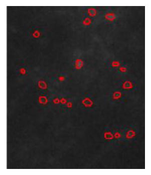	Patch 3	Patch 4
Score	1.01	0.98	1.02	0.95	2.54	1.54	0.97	0.12
Source					Image 1	Image 2	Image1	Image2
Remark					High vesicle density region	High vesicle density region	Average vesicle density region with bright spots	Low density vesicle region

Table 4 shows that there are no obvious differences between four images with similar vesicle density. Patches 1 and 2 are cropped from Images 1 and 2, representing cases with high a density of vesicles. Patch 3 illustrates the image with an average number of vesicles. Patch 4 contains a limited number of vesicles. Patch 3 also includes several bright spots which are not vesicles but noise. All four cropped patches have the same image size. As expected, high vesicle density Patches 1 and 2 have higher scores. Due to the nature of the score, the higher the vesicle density, the more active are the neurons. This positive correlation relation holds between the score and the intensity difference between before and after stimulation.

In this work, we do not provide a score benchmark because different data batches have varying neuron density and intensity conditions. It is not appropriate to assign a global threshold to distinguish active and non-active neurons for data generated for different purposes. With scores provided by the pipeline, biologists can simply set a threshold for each case according to their research objectives.

Parameter settings

Since several parameters are employed in this work, we briefly discuss the parameter setting issue here. For MSVST enhancement, we followed the standard parameter configuration described by Zhang et al., 2008. To achieve balance between false positives and negatives, we set the threshold on the enhanced map at two. In adaptive thresholding, the lower boundary of candidate vesicle region size is set to five. Parameters used in post processing were discussed in the Methods section. All parameters are derived from a large number of experiments. Most of them are robust and can be fixed loosely within a range. The size of vesicles and the shrinkage or expansion of the radius will vary from case to case because vesicles can be imaged at different facilities and resolutions. Here, we use relative information as much as possible (such as the difference between an image pair and the ratio of changes instead of absolute values); this enables the proposed robust strategy to be applied to different data sets. The average running time to process a 512×512 pixel image is less than a minute on a Xeon 3.0G Hz processor workstation with 4GB RAM.

Discussion

To measure neuron activity, we consider the total intensity difference of vesicles divided by the area of the image data. In this scoring system, the number of vesicles, the sum of the average intensity of each vesicle, and the size of image data influence the activity score. Since we extracted various features from the vesicles, it might be possible to incorporate more features into the scoring system. For example, we can include the regression coefficients or soft classification coefficients into the score if the supervised method is employed. Other features, such as wavelet coefficients, are not appropriate for introduction to the scoring system because it is difficult to explain neuron activity with abstract numbers in a transformed domain. For the same reason, features in the moment group are difficult to directly connect to neuron activity with biological meaning.

Although the proposed unsupervised methods achieve desired results, there is still a possibility of improving the detection result by employing more sophisticated machine learning strategies. A potential choice is online SVM (Bordes, Ertekin et al. 2005). Rather than batch learning problems, online SVM updates the classifier with new samples and new labels. We can include high confidence data in each learning step and update the classifier to achieve better accuracy. In addition, some features can be generated and updated during the online learning processing. For example, as we noted earlier, vesicles tend to cluster in a neighborhood, as do dead spots. Therefore, we can count the number of both positive and negative training samples in the neighborhood region of a given spot. This information can be updated after each learning step and also can be used in the classifier to obtain the support vector. Although online SVM and other semi-supervised SVM may achieve better classification accuracy, these methods suffer lengthy processing time and frequent human intervention. In our future work, we will aim to achieve a balance between accuracy and time-consumption together with human effort.

The final issue is the robustness of the proposed system. PSNR (peak signal-to-noise ratio) is an important criterion for quantifying the image quality as well as a measurement of system robustness. In order to find the lower boundary of image quality, we calculate the PSNR of the original data and images contaminated by additive Gaussian noise. Fig. 13 illustrates that, for Image 1, the PSNR decreases while the Gaussian noise variance level increases. The proposed system is able to identify about 70% of the spots detected in the added-noise-free version when the Gaussian noise variance increased to 1e-3. This corresponds to a cut-off value of PSNR at 33 dB.

Fig. 13.

PSNR of Image 1 contaminated by Gaussian noise.

Conclusions

Synaptic vesicles are involved in performing presynaptic functions. The synapse assay can be implemented in a high throughput manner via automated, multi-well plate microscopy to study neuron activity and to do drug screening in neurodegradation diseases. For the large amount of image data generated by large scale experiments, automated processing and statistical analysis of the synaptic vesicle image will provide significant statistical power and save biologists from manually labeling and counting vesicles. However, to our knowledge, such quantization tools designed specifically for high throughput synaptic vesicle assays do not exist.

In this paper, we presented a neural image quantization pipeline to analyze a synaptic vesicle neuron image stained by FM dye. We can detect active vesicles releasing the neurotransmitter, FM dye in this case, to measure the neuron activity. This pipeline is fully automated, time efficient, and ready for batch processing. We address the inhomogeneity issue by introducing local adaptive threshold on a MSVST enhanced map. This method is robust to detect both vesicles with high intensity background and weak vesicles with low intensity. In addition, we develop novel strategy to solve the overlapped spots issue for tiny objects such as synaptic vesicles. Several criteria have been proposed to remove various categories of undesired structures. When compared with a popular supervised method, the proposed pipeline provides better detection accuracy and time efficiency. With detection and segmentation results, we extract different types of image features to quantify each detection vesicle. These features include intensity, intensity change between before and after stimulation, perimeter, convexity, and other texture features, moment features, and wavelet coefficients. Finally, a quantified score is provided for each input image to measure the activity of the neuron in a whole image. This score allows the statistical quantification of the neuron activity, which is measured by differences between before and after stimulation. To summarize, we develop an automated, batch processing-ready, and cost-effective pipeline to measure the neuron activity based on the synaptic vesicle image data used in neurodegenerative disease research, which will help neuroscientists and researchers analyze high-throughput imaging data in neuropathology studies and drug screening.

References

- Abramov E, Dolev I, et al. Amyloid-beta as a positive endogenous regulator of release probability at hippocampal synapses. Nat Neurosci. 2009;12(12):1567–1576. doi: 10.1038/nn.2433. [DOI] [PubMed] [Google Scholar]
- Besl PJ, McKay ND. IEEE Transactions on pattern analysis and machine intelligence. 1992. A method for registration of 3-D shapes; pp. 239–256. [Google Scholar]
- Betz WJ, Bewick GS. Optical analysis of synaptic vesicle recycling at the frog neuromuscular junction. Science. 1992;255(5041):200–203. doi: 10.1126/science.1553547. [DOI] [PubMed] [Google Scholar]
- Boland MV, Markey MK, et al. Automated recognition of patterns characteristic of subcellular structures in fluorescence microscopy images. Cytometry. 1998;33(3):366–375. [PubMed] [Google Scholar]
- Bordes A, Ertekin S, et al. Fast kernel classifiers with online and active learning. The Journal of Machine Learning Research. 2005;6:1579–1619. [Google Scholar]
- Chang CC, Lin CJ. LIBSVM: a library for support vector machines. 2001. [Google Scholar]
- Cheung ZH, Fu AK, et al. Synaptic roles of Cdk5: implications in higher cognitive functions and neurodegenerative diseases. Neuron. 2006;50(1):13–18. doi: 10.1016/j.neuron.2006.02.024. [DOI] [PubMed] [Google Scholar]
- Cochilla AJ, Angleson JK, et al. Monitoring secretory membrane with FM1-43 fluorescence. Annu Rev Neurosci. 1999;22:1–10. doi: 10.1146/annurev.neuro.22.1.1. [DOI] [PubMed] [Google Scholar]
- Cortes C, Vapnik V. Support-vector networks. Machine learning. 1995;20(3):273–297. [Google Scholar]
- Dejnozkova E, Dokladal P. Modelling of overlapping circular objects based on level set approach. Image Analysis and Recognition. 2004:416–423. [Google Scholar]
- Dreosti E, Lagnado L. Optical reporters of synaptic activity in neural circuits. Exp Physiol. 2011;96(1):4–12. doi: 10.1113/expphysiol.2009.051953. [DOI] [PubMed] [Google Scholar]
- Esposito G, Fernandes AC, et al. Synaptic vesicle trafficking and Parkinson’s disease. Dev Neurobiol. 2011 doi: 10.1002/dneu.20916. [DOI] [PubMed] [Google Scholar]
- Fan J, Zhou X, et al. An automated pipeline for dendrite spine detection and tracking of 3D optical microscopy neuron images of in vivo mouse models. Neuroinformatics. 2009;7(2):113–130. doi: 10.1007/s12021-009-9047-0. [DOI] [PMC free article] [PubMed] [Google Scholar]
- Feichtinger HG, Strohmer T. Gabor analysis and algorithms: Theory and applications. Birkhauser; 1998. [Google Scholar]
- Gaffield MA, Betz WJ. Imaging synaptic vesicle exocytosis and endocytosis with FM dyes. Nat Protoc. 2006;1(6):2916–2921. doi: 10.1038/nprot.2006.476. [DOI] [PubMed] [Google Scholar]
- Gonzalez RC, Woods RE. Digital image processing. Upper Saddle River, NJ: Pearson/Prentice Hall; 2008. [Google Scholar]
- Hann MM, Oprea TI. Pursuing the leadlikeness concept in pharmaceutical research. Curr Opin Chem Biol. 2004;8(3):255–263. doi: 10.1016/j.cbpa.2004.04.003. [DOI] [PubMed] [Google Scholar]
- Jung C, Kim C, et al. Unsupervised segmentation of overlapped nuclei using Bayesian classification. IEEE Trans Biomed Eng. 2010;57(12):2825–2832. doi: 10.1109/TBME.2010.2060486. [DOI] [PubMed] [Google Scholar]
- Li C, Kao CY, et al. Minimization of region-scalable fitting energy for image segmentation. Image Processing, IEEE Transactions on. 2008;17(10):1940–1949. doi: 10.1109/TIP.2008.2002304. [DOI] [PMC free article] [PubMed] [Google Scholar]
- Li X, Lebonvallet S, et al. An improved level set method for automatically volume measure: application in tumor tracking from MRI images. Conf Proc IEEE Eng Med Biol Soc. 2007;2007:808–811. doi: 10.1109/IEMBS.2007.4352413. [DOI] [PubMed] [Google Scholar]
- Moretti P, Levenson JM, et al. Learning and memory and synaptic plasticity are impaired in a mouse model of Rett syndrome. J Neurosci. 2006;26(1):319–327. doi: 10.1523/JNEUROSCI.2623-05.2006. [DOI] [PMC free article] [PubMed] [Google Scholar]
- Rakotomamonjy A. Variable selection using svm based criteria. The Journal of Machine Learning Research. 2003;3:1357–1370. [Google Scholar]
- Rizzoli SO, Betz WJ. The structural organization of the readily releasable pool of synaptic vesicles. Science. 2004;303(5666):2037–2039. doi: 10.1126/science.1094682. [DOI] [PubMed] [Google Scholar]
- Selkoe DJ. Alzheimer’s disease is a synaptic failure. Science. 2002;298(5594):789–791. doi: 10.1126/science.1074069. [DOI] [PubMed] [Google Scholar]
- Sudhof TC. The synaptic vesicle cycle. Annu Rev Neurosci. 2004;27:509–547. doi: 10.1146/annurev.neuro.26.041002.131412. [DOI] [PubMed] [Google Scholar]
- Wang J, Zhou X, et al. An image score inference system for RNAi genome-wide screening based on fuzzy mixture regression modeling. J Biomed Inform. 2009;42(1):32–40. doi: 10.1016/j.jbi.2008.04.007. [DOI] [PMC free article] [PubMed] [Google Scholar]
- Wang M, Zhou X, et al. Novel cell segmentation and online SVM for cell cycle phase identification in automated microscopy. Bioinformatics. 2008;24(1):94–101. doi: 10.1093/bioinformatics/btm530. [DOI] [PubMed] [Google Scholar]
- Yan P, Zhou X, et al. Automatic segmentation of high-throughput RNAi fluorescent cellular images. IEEE Trans Inf Technol Biomed. 2008;12(1):109–117. doi: 10.1109/TITB.2007.898006. [DOI] [PMC free article] [PubMed] [Google Scholar]
- Zeng Q, Miao Y, et al. Algorithm based on marker-controlled watershed transform for overlapping plant fruit segmentation. Optical Engineering. 2009;48:027201. [Google Scholar]
- Zhang B, Fadili JM, et al. Wavelets, ridgelets, and curvelets for Poisson noise removal. IEEE Trans Image Process. 2008;17(7):1093–1108. doi: 10.1109/TIP.2008.924386. [DOI] [PubMed] [Google Scholar]
- Zhou X, Li F, et al. A novel cell segmentation method and cell phase identification using Markov model. IEEE Trans Inf Technol Biomed. 2009;13(2):152–157. doi: 10.1109/TITB.2008.2007098. [DOI] [PMC free article] [PubMed] [Google Scholar]
- Zoghbi HY. Postnatal neurodevelopmental disorders: meeting at the synapse? Science. 2003;302(5646):826–830. doi: 10.1126/science.1089071. [DOI] [PubMed] [Google Scholar]