Dissociation of Response Variability from Firing Rate Effects in Frontal Eye Field Neurons during Visual Stimulation, Working Memory, and Attention

Abstract

Recent studies suggest that trial-to-trial variability of neuronal spiking responses may provide important information about behavioral state. Observed changes in variability during sensory stimulation, attention, motor preparation, and visual discrimination suggest that variability may reflect the engagement of neurons in a behavioral task. We examined changes in spiking variability of frontal eye field (FEF) neurons in a change detection task requiring monkeys to remember a visually cued location and direct attention to that location while ignoring distracters elsewhere. In this task, the firing rates (FRs) of FEF neurons not only continuously reflect the location of the remembered cue and select targets, but also predict detection performance on a trial-by-trial basis. Changes in FEF response variability, as measured by the Fano factor (FF), showed clear dissociations from changes in FR. The FF declined in response to visual stimulation at all tested locations, even in the opposite hemifield, indicating much broader spatial tuning of the FF compared with the FR. Furthermore, despite robust spatial modulation of the FR throughout all epochs of the task, spatial tuning of the FF did not persist throughout the delay period, nor did it show attentional modulation. These results indicate that changes in variability, at least in the FEF, are most effectively driven by visual stimulation, while behavioral engagement is not sufficient. Instead, changes in variability may reflect shifts in the balance between feedforward and recurrent sources of excitatory drive.

Introduction

Recent studies suggest that trial-to-trial variability of neuronal spiking responses may provide information about behavioral and cognitive states. By itself, sensory stimulation elicits a decline in response variability throughout many cortical areas, regardless of behavioral context and whether or not a receptive field (RF) stimulus evokes a change in firing rate (FR) (Churchland et al., 2010), suggesting that sensory input drives local network activity to a stable state. In addition, changes in response variability have also been observed as a correlate of active behavioral states. Variability in visual cortex decreases with attention to a RF stimulus, indicating improved reliability of selected sensory representations (Mitchell et al., 2007; Cohen and Maunsell, 2009). Declines in variability during motor preparation, such as in dorsal premotor cortex for visually guided arm reaches (Churchland et al., 2006) and in visual cortex for visually guided saccades (Steinmetz and Moore, 2010), predict movement reaction time better than FR, suggesting that networks converge to a stable state before movement execution (Churchland et al., 2007).

The frontal eye field (FEF) is known to be involved in visually guided saccadic eye movements (Bruce and Goldberg, 1985), and FEF neurons exhibit spatially selective persistent activity during tasks in which monkeys make delayed saccades to previously cued spatial locations (Bruce and Goldberg, 1985; Sommer and Wurtz, 2000). The FEF has also been implicated in the control of covert spatial attention (Moore and Fallah, 2001; Noudoost et al., 2010). Even in the absence of saccade preparation, FEF neurons exhibit working memory-related delay activity that is linked to successful deployment of attention (Armstrong et al., 2009). In a task requiring monkeys to remember a location and direct attention to it while ignoring distracters, the FR of FEF neurons maintains a continuous representation of the remembered location. During the delay period, neurons exhibit spatially selective persistent activity that correlates with subsequent selection of the target stimuli during the array flashes. Furthermore, the FR predicts performance of the monkey on a trial-by-trial basis. Given the clear behavioral engagement of monkeys in the task and the robust visual and cognitive FR modulation of FEF neurons, one might expect the spiking variability of those neurons to also reflect components of the task.

We compared changes in FR and trial-to-trial spiking variability, as measured by the Fano factor (FF), across six cue locations for all epochs in the task and found clear dissociations between the two measures, indicating that effects in FF do not just mirror changes in FR. The FF declined with visual stimulation at all tested locations, even in the opposite hemifield, indicating much broader spatial tuning of the FF compared with the FR. However, during the delay period, the FF returned to baseline levels despite the robust spatially selective persistent activity. Spatial tuning of the FF during the flashes was absent as well, despite attentional modulation of the FR. Thus, declines in FF, at least in the FEF, appear to be most effectively driven by visual stimulation, and the degree of arousal or engagement of the network is not sufficient to drive changes in variability. Instead, changes in response variability may reflect shifts in the balance between feedforward and recurrent sources of excitatory drive.

Materials and Methods

Subjects.

Two male monkeys (Macaca mulatta; 7 and 12 kg) were used in these experiments. All experimental procedures were in accordance with National Institutes of Health Guide for the Care and Use of Laboratory Animals, the Society for Neuroscience Guidelines and Policies, and Stanford University Animal Care and Use Committee. General surgical procedures have been described previously (Armstrong et al., 2006).

Visual stimuli and behavior.

Visual stimuli, behavioral tasks, and physiological recordings have been described previously (Armstrong et al., 2009). Throughout the experimental session, monkeys were seated in a primate chair equipped with a manual response lever. For all experiments, eye position was monitored with a scleral search coil with a spatial resolution of ≪0.1° (Armstrong et al., 2006) and was digitized at 200 Hz. Figure 1 illustrates the behavioral task and the setup for recording. Monkeys were trained to maintain fixation on a 0.6° diameter central spot within a 2.3–4.9° diameter error window throughout the duration of the task and depress the lever to initiate an experimental trial. Breaks in fixation before the trial was completed were considered aborted trials and were not included in the data analysis. A total of 50–515 ms after the monkey's initiation of a trial, a circular cue stimulus (1.2° diameter) was presented for 120–270 ms (Cue epoch), indicating the target location in an upcoming array, followed by a delay period of 600–1600 ms (Delay Period epoch). For a given experimental block, the length of the delay period remained constant. At the end of the delay, a circular array comprised of six circular square-wave grating stimuli (2.5–4° diameter; 0.71–0.91 cycles/degree; 0.49–0.95 Michaelson contrast) was flashed twice. The first array was flashed for 285–290 ms (flash 1), followed by a 120–235 ms period during which only the fixation point remained on the screen [interflash interval (IFI)], and then the array was flashed a second time for 270 ms (flash 2). If the target grating changed orientation (20–90° rotation) between the two flashes of the array (change condition), monkeys were required to release the lever within 600 ms (monkey 1) or 1000 ms (monkey 2) following the onset of flash 2 to receive a juice reward. By contrast, if the target item did not change orientation between the two flashes (no-change condition), the monkeys were required to continue to depress the lever throughout the response window to be rewarded. A subset of uncued “probe” trials, occurring on randomly selected trials with a frequency of 0–10% for a given experiment, were included to test the dependence of behavioral performance on the cue. Probe trials had identical event timing as normal experimental trials; however, on the probe trials, the cue was not presented, and the screen was left blank during this interval. Performance on these interleaved trials in which the cue was omitted was significantly worse than for trials in which a spatial cue was given, confirming that the spatial cue was used to direct attention to the target location (Armstrong et al., 2009). Neuronal responses on probe trials were excluded from the data analyses reported here.

Figure 1.

Experimental setup. A, Change detection task. The monkey maintained fixation throughout the duration of the trial. To initiate a trial, the monkey depressed a manual lever, and, after a few hundred milliseconds, a peripheral cue was presented briefly, indicating the target location. After a fixed delay period, an array of six oriented gratings was flashed twice. On trials in which the target stimulus changed orientation across flashes (change trial), the monkey was rewarded for releasing the lever. On trials in which the target stimulus did not change (no-change trial), the monkey was rewarded for continuing to hold the lever for an additional 600–1000 ms. All six locations were equally likely to be cued, and the cue was 100% valid. B, Stimulus alignment. The FEF RF for each recording site was determined before running the change detection task by applying microstimulation (< 50 μA) during a simple fixation task and mapping the evoked saccades. An example set of eye traces from microstimulation-evoked saccades are shown. The array of gratings was positioned such that one grating was centered at the average evoked saccade endpoint. C, Trials in which the monkey was cued to attend to the RF are labeled “Cue RF,” whereas trials in which the monkey was cued to attend to the opposite array location are labeled “Cue away.”

On a given trial, a cue was equally likely to appear at any of the six array locations, and change and no-change trials were equally likely to occur. Each stimulus in the array was oriented at one of two angles, orientation A or orientation B, determined before the start of the experiment. On each trial, the orientations of the five distracter gratings were randomly assigned to either orientation A or B. The target grating was assigned to orientation A on one-half of the trials, and orientation B on the other one-half of trials. On change trials, the second flash of the target grating changed orientations (either A to B, or B to A), whereas for no-change trials the target grating remained the same. Orientation changes only occurred at the target location. All cue location, change and no-change, and target orientation conditions were pseudorandomly interleaved and were controlled by the CORTEX system for data acquisition and behavioral control. Each array stimulus was equidistant from the fixation point (3.6–16.8° visual angle), and each stimulus was separated from its neighbors by 60° θ. During each experiment, the array was adjusted so that one stimulus was positioned inside the RF of the FEF neuron being recorded. All visual stimuli were displayed on an LCD monitor. Stimulus presentation was controlled and recorded by CORTEX, and the timing of stimulus onset and offset events was confirmed with a photodiode.

Neural recordings.

Single-neuron recordings in awake monkeys were made through a surgically implanted cylindrical titanium chamber (20 mm diameter) overlaying the arcuate sulcus. Electrodes were lowered into the cortex using a hydraulic microdrive (Narashige). Activity was recorded extracellularly with varnish-coated tungsten microelectrodes (FHC) of 0.2–1.0 MΩ impedance (measured at 1 kHz). Extracellular waveforms were digitized and classified as single neurons using both template-matching and window-discrimination techniques either on-line or off-line (Plexon). During each experiment, a recording site in the FEF was first localized by the ability to evoke fixed-vector, saccadic eye movements with stimulation at currents of <50 μA (Bruce et al., 1985). During each experimental session, we mapped the saccade vector elicited via microstimulation at the cortical site under study with a separate behavioral paradigm (Moore and Fallah, 2001). In this paradigm, the monkey was required to fixate on a visual stimulus (0.48° diameter circle) for 500 ms, after which time a 100 ms stimulation train was delivered on one-half of the trials. For each trial, the visual stimulus was positioned at one of five locations, one at the center of gaze and one 10–13° from center along each cardinal direction. Evoked saccades had vectors with lengths ranging from 3.6 to 14.4° visual angle, and angles of 120–270° θ. After mapping the saccade vector, we recorded the response of any neuron that could be isolated by advancing the electrode within 0–900 μm of the stimulation site (average distance from stimulation site was 125 μm) while monkeys performed the change detection task. The array was adjusted so that one stimulus was presented inside the RF of the FEF neuron (Fig. 1B). This configuration allowed us to examine FEF neuron responses on trials in which the monkey was cued to direct attention to the stimulus appearing inside the RF of the FEF neuron (Cue RF condition) compared with when the cue appeared at the opposite array location (180° θ away, in the opposite hemifield), indicating that the monkey should direct attention away from the RF of the FEF neuron (Cue away condition) (Fig. 1C).

Data analysis.

All analyses were performed in MATLAB (MathWorks). Activity was analyzed by sliding a 150 ms window in 5 ms steps across the spike train data. Only data from completed trials with correct responses were included in the analyses. At each time point in the delay, only trials with delay lengths that included the specified time window were included. Normalized population response (FR) histograms were computed by dividing responses in each time bin by the peak average response across all time bins and conditions for individual neurons and then averaging across neurons. Trial-to-trial variability, as measured by the FF, was calculated as the ratio of the variance to the mean of spike counts across trials within each 150 ms time window. The FF was calculated separately for each condition and individual neuron and then averaged across neurons. The length of the delay period remained constant within an experimental block. Neuronal recordings for which the delay length was shorter than the analyzed window were excluded (e.g., neurons recorded with a short delay period of 600 ms were not included at the 1000 ms time point). The reported results for the full population remained comparable using only the subset of trials with long delay periods.

Modulation of both the FR and FF was assessed using a number of metrics. Conditions were grouped according to the location of the cue, in terms of the radial distance from the RF. To compare the condition in which the monkey was cued to attend the RF (Cue RF) with the condition in which the monkey was cued to attend the opposite array location (Cue away), a sliding analysis window, incremented every 10 ms, was used to determine intervals of significant difference between the Cue RF and Cue away condition (Wilcoxon's signed rank, p < 0.01), significant difference between the Cue RF condition and baseline (Wilcoxon's signed rank, p < 0.01), and significant difference between the Cue away condition and baseline (Wilcoxon's signed rank, p < 0.01). To quantify the magnitude of tuning across opposite cue locations, a spatial tuning index (STI) was calculated. The STI was computed as follows:

where y represents either the FR or FF. The STI was computed for individual neurons and then averaged across the population. The average STI was also converted to a spatial tuning ratio (STR), using the following:

where ȳ represents the population average of the FR or FF and STI represents the average STI across neurons. The STR was converted from the average STI rather than computed from individual neurons.

Tuning functions were constructed to examine difference in FR and FF across all six cue locations, using representative 150 ms analysis windows within each epoch: baseline (−150 to 0 ms before cue onset), cue (50–200 ms after cue onset), middle of the delay period (400–550 ms after cue offset), late in the delay period (1400–1550 ms after cue offset), first flash (50–200 ms after flash 1 onset), IFI (50–200 ms after flash 1 offset), and second flash (50–200 ms after flash 2 offset). Spatial modulation of the FR and FF was assessed using a separate set of metrics. To determine the significance of deviation of FR or FF from baseline for individual cue conditions during each epoch, a Wilcoxon's signed-rank test was used with a significance level of p < 0.05. The equality of population mean values across all six cue locations was measured using a repeated-measures ANOVA. In some cases in which the average FR was zero, the resulting FF was infinite and excluded from the population average. While the plotted population tuning curves with SEs include all finite values, only neurons with finite values for both FR and FF curves across all six locations were included in the repeated-measures ANOVA. All subsequent uses of the term “ANOVA” refer to a repeated-measures ANOVA. For tuning functions that yielded a significant ANOVA or STI result (p < 0.01), a von Mises, or circular Gaussian, function was used to fit a continuous tuning curve to the six population mean values using a nonlinear least-squares optimization (lsqcurvefit in MATLAB). The von Mises function was defined as follows:

where θ is the radial angle from the RF of the neuron in radians, μ determines the offset of the center from 0°, κ determines the width of the function (with larger values of κ representing narrower curves), A scales the amplitude, and c adds a constant offset for the base of the circular Gaussian. To avoid overfitting, the displacement of the peak of the function, μ, was restricted to ±10°. In the data, tuning functions for the FF were inverted (upside down) compared with the FR, and to maintain a consistent measure of the bandwidth for both functions, the width parameter was constrained to be positive (κ > 0). Negative values of κ result in inverted curves, so by constraining κ to be positive, the sign of all fitted functions was reflected only in the sign of the amplitude (A) term. For each parameter, 95% confidence intervals (CI₉₅) were estimated using a bootstrapping procedure (Efron, 1979). The population of neurons was resampled 500 times with replacement to calculate the averages for each cue condition, and the subsequent average was fit to the von Mises function. The confidence intervals were taken as the 5th and 95th percentile values for each parameter. Goodness of fit was measured by calculating an R² for each tuning curve fit. The tuning bandwidth was defined as the full width at half-maximum (FWHM), which was computed from the κ parameter of the von Mises fit, using the following formula (Elstrott et al., 2008):

Functional subpopulations were defined based on responsiveness to a cue presented in the RF and spatial selectivity during the delay. Visual responsiveness was defined as significantly higher average firing rate during the first 100 ms of the cue presentation (offset by a 50 ms visual latency) compared with the 200 ms baseline preceding the onset of the cue (Wilcoxon's rank sum, p < 0.05). Delay selectivity was defined as significant difference in average activity between the Cue RF and Cue away conditions during the last 400 ms of the delay period (p < 0.05). For statistical significance, p values <10⁻⁷ are reported as p < 10⁻⁷. Unless otherwise stated, statistics reported in Results are based on a Wilcoxon's signed-rank test.

Results

FEF neuron responses and response variability

We recorded the activity of 126 FEF neurons (monkey 1, 56 neurons; monkey 2, 70 neurons). Figure 2 shows the time courses of the normalized FR and FF, averaged over the population, for trials in which the cue appeared in the RF compared with trials in which the cue appeared in the opposite array location. In this task, all trials were visually indistinguishable after the presentation of the cue, but the FR of neurons differentiated between the Cue RF and Cue away conditions, starting from the onset of the cue and continuing throughout the remainder of the trial. Figure 2A shows the average normalized FR of the population of FEF neurons for both Cue RF and Cue away trials. At the onset of a brief cue presentation in the RF, FEF neurons exhibited a large, transient increase in FR (Cue RF vs baseline, p < 10⁻⁷). When the cue appeared away from the RF (in the opposite hemifield), the population average did not show a significant visual response (Cue away vs baseline, p > 0.23). After the disappearance of the cue in the RF, neurons sustained an elevated level of activity throughout the delay (p < 0.0003), while after a cue away, activity was initially suppressed compared with baseline (p < 10⁻⁵ until 400 ms after the offset of the cue) and remained near baseline later in the delay period (p > 0.01). In the second phase of the trial, in which the monkey must attend to the cued location to correctly identify a target stimulus change, the two stimulus array flashes each evoked a transient increase in the FR for both cue conditions (p < 10⁻⁷ compared with baseline). Despite an overall increase in FR due to equivalent stimulation in all conditions, the FR remained spatially modulated throughout both flashes (Cue RF vs Cue away, p < 0.01). Between array flashes, the FR in both cue conditions declined but still remained separated (p < 0.01), as the FR on Cue RF trials remained well above baseline (p < 10⁻⁷) and the FR on Cue away trials remained slightly above baseline (p < 0.01). The FR maintained a consistent representation of the cued location throughout the trial, exhibiting persistent activity in epochs without visual stimulation and spatially modulated visual responses during the stimulus array presentations.

Figure 2.

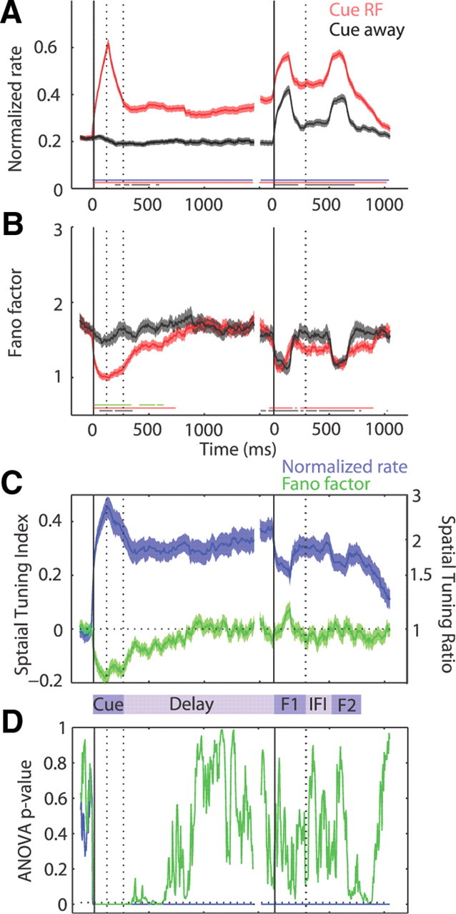
Time course of FR and FF. A, Average normalized FR of 126 FEF neurons, in a sliding 150 ms window, aligned to the onset of the cue (left solid vertical line) and the onset of the first presentation of the stimulus array (right solid vertical line) on correct trials in which the monkey was cued to attend to the RF location (red) and cued to attend away (gray). The vertical dotted lines indicate the range of offset times for the cue and first flash. Only no-change trials are included on the right. The thin lines along the bottom of the plot show intervals of significance, stepped every 10 ms: blue represents significant difference between the Cue RF and Cue away condition, red represents significant difference between the Cue RF condition and baseline, and black represents significant difference between the Cue away condition and baseline (Wilcoxon's signed rank, p < 0.01 for each). B, Corresponding FF. Conventions are the same as above, except the thin green line represents intervals of significant difference between the Cue RF and Cue away condition. C, Average STI for FR (blue) and FF (green), calculated using the respective values in Cue RF and Cue away conditions. Corresponding STR values on the secondary y-axis on the right were converted from the average STI values. The horizontal dotted line marks the zero value. D, Repeated-measures ANOVA p value for the FR (blue) and FF (green) values across all six cue locations. The horizontal dotted line marks 0.05 for reference. Error bars indicate SEM. F1, Flash 1; IFI, interflash interval; F2, flash 2.

In contrast to the FR, the FF transiently declined with each stimulus presentation but only exhibited spatially specific modulation during the cue presentation. The FF showed a greater decline when a stimulus was presented in the RF compared with the opposite array location. Figure 2B shows the time course of the average FF throughout the task for both Cue RF and Cue away conditions. The FF showed a sharp decline from its baseline value of ∼1.7 to a value near 1 in response to a cue presented in the RF (p < 10⁻⁷). When a cue was presented in the opposite location, the FF showed a smaller but still significant decline to ∼1.5 (p < 10⁻³). After the offset of a cue presented in the RF, the FF decayed back to baseline by 540–600 ms into the delay period (p < 0.01 until 540 ms and p < 0.05 until 600 ms). In contrast, after the offset of a cue presented in the opposite location, the FF was indistinguishable from baseline and remained this way throughout the delay (p > 0.01). During the array flashes, the FF declined for both Cue RF and Cue away conditions (p < 10⁻⁷). However, unlike the FR, the magnitude of the decline in FF during the array flashes remained indistinguishable between cue conditions (p > 0.01). Between array flashes, the FF rebounded but still remained significantly below baseline (p < 0.01) and lacked spatial tuning (p > 0.01). The FF consistently reflected the presence of a stimulus on the screen, but unlike the FR, the FF did not maintain a representation of the cued location throughout the trial.

To quantify the degree of spatial selectivity throughout the trial, we first calculated a running STI for both measures, as plotted in Figure 2C. Both STI_FR and STI_FF curves started at zero during baseline. Deviations from zero in either direction in subsequent task epochs indicate spatially specific modulation. With the onset of the cue, the STI_FR rose from zero to ∼0.45, or equivalently, the FR response to a cue in the RF was >2.5 times the response to a cue appearing in the opposite hemifield (p < 10⁻⁷). Similarly, at the onset of the cue, the STI_FF declined from zero to approximately −0.17, meaning the FF decline was ∼1.4 times greater for a cue presented in the RF compared with a cue presented in the opposite hemifield (p < 10⁻⁷). After the transient visual response to the cue, the STI_FR remained ∼0.35 throughout the delay, corresponding to a FR during Cue RF trials that was approximately two times the response during Cue away trials (STR_FR ≈ 2; p < 10⁻⁷). In contrast, the STI_FF decayed to within 0.05 of zero by 550 ms after the offset of the cue, corresponding to a FF that differed by <10% between Cue RF and Cue away trials. In the latter part of the trial, the STI_FR remained well above zero, showing declines during both flashed array presentations to ∼0.2 and a slight recovery between flashes to ∼0.3 (STI_FR, p < 10⁻⁷ for all three epochs). Thus, despite the large spatial modulation in the FR, the FF did not show spatial modulation throughout the remainder of the trial (STI_FF, p > 0.02). Figure 2D shows the statistical tuning of the FR and FF over time using all six cue conditions (including Cue RF and Cue away), as measured by the p value of an ANOVA performed at each time point. This plot confirms the difference in spatial tuning between the FR and FF with tuning of the FR remaining consistent throughout the trial and tuning of the FF decaying into the delay period. Both the population FR and FF reliably indicated the presence of an RF stimulus, but only the FR maintained spatial information throughout the trial and selected the target stimulus among distracters during the flashed array presentations.

Spatial tuning across epochs

To characterize the dynamics of spatial modulation of the FF and FR throughout the trial, we examined responses from conditions in which the cue was presented at each of the six possible radial locations. Figure 3 shows the population spatial tuning curves for FR and FF across all epochs of the task, using seven representative analysis windows. Each data point represents the average normalized FR or average FF as a function of radial location relative to the RF in a 150 ms time window during each epoch of the task: baseline, cue, mid-delay (400 ms after the cue offset), late-delay (1400 ms after the cue offset), flash 1, IFI, and flash 2. For functions that were significantly tuned (ANOVA or STI, p < 0.01), curve fitting with a von Mises (circular Gaussian) function was applied to the population average values to parameterize the tuning functions in terms of amplitude (A), tuning width measured as FWHM, and constant offset (c).

Figure 3.

Spatial tuning across all task epochs. A, B, Average normalized FR (A) and FF values (B) as a function of radial distance from the RF location for 150 ms windows during the baseline, cue, 400 ms into the delay, 1400 ms into the delay, first flash, interflash interval, and second flash. The box panels along the top show a schematic diagram of the display seen by the monkey during each task epoch. The horizontal magenta lines below the schematic timeline and connected to each box panel indicate the 150 ms window used for analysis (baseline, −150 to 0 ms before cue onset; cue, 50–200 ms after cue onset; delay, 400–550 and 1400–1550 ms after cue offset; flash 1, 50–200 ms after flash 1 onset; IFI, 50–200 ms after flash 1 offset; flash 2, 50–200 ms after flash 2 offset). Each point represents the average FR or FF value for the corresponding cue location, and error bars denote the SEM. The dotted lines represent the average baseline value across all six cue locations, and the black outlined points indicate significant deviation from baseline (Wilcoxon's signed rank, p < 0.05). For each tuning function, if the points were spatially tuned, as determined by an ANOVA (p < 0.01), the average values for each location were fit to a von Mises, or circular Gaussian function, shown by a continuous solid line. Functions that were not significantly tuned according to the ANOVA are shown with a dashed line across the mean of the average values across all locations.

Figure 3A shows spatial tuning curves for the FR during each epoch of the task, and Table 1 shows corresponding tuning curve fit parameters. The FR exhibited consistently high spatial tuning throughout all epochs of the trial starting from the onset of the cue (ANOVA, p < 10⁻⁷). Curve fitting with von Mises functions provided good fits for the FR tuning curves (R² > 0.96), with a positive peak centered around the RF (μ = ±10°; as constrained by the fit optimization) and a narrow bandwidth (FWHM_FR = 70–77°). Strong spatial tuning arose during the cue epoch as the FR increased significantly above baseline in response to a cue presented at locations within and immediately surrounding the RF (θ = −60°: p < 0.02; 0°: p < 10⁻⁷; 60°: p < 0.006), but remained near or below baseline in response to a cue presented at more distant locations (−120°: p < 0.03; 120°, 180°: p > 0.1), resulting in a narrow tuning curve with a base near the average baseline FR (c_FR: p > 0.05). During the delay period when no stimulus was present, the spatial tuning diminished in amplitude but was still clearly present (A_FR: p < 0.05 compared with cue epoch, p < 0.05 compared with zero). The FR on trials in which the monkey was cued to attend the RF location remained significantly above baseline (p < 0.04), while the FR on trials in which the monkey was cued to attend a location immediately surrounding the RF returned to baseline (θ = −60, 60°: p > 0.1), and the FR on trials in which the monkey was cued to attend more distant locations decreased below baseline (θ = −120, 120, 180°: p < 0.008). The fitted tuning curves remained comparably narrow (FWHM_FR: p > 0.05 compared with cue epoch) with a base near the average baseline FR (c_FR: p > 0.05). During the first flash presentation, the entire tuning curve shifted above baseline (c_FR: p < 0.05) as the FR increased above baseline for all cue conditions (p < 10⁻⁷). Despite an overall increase in FR across all conditions, the FR still maintained spatial selectivity similar to the preceding delay period (A_FR, FWHM_FR: p > 0.05). During the IFI, the tuning curve shifted down (c_FR: p < 0.05) but remained above the baseline FR (c_FR: p < 0.05), as the FR for most cue conditions remained above baseline (p < 0.01, except at 60°: p > 0.06), and spatial selectivity persisted (A_FR, FWHM_FR: p > 0.05 compared with F1). During the second flash presentation, the neurons again responded with an overall increase in FR for all cue conditions (p < 10⁻⁶ compared with baseline), leading to another upward shift in the entire tuning curve (c_FR: p < 0.05 compared with IFI) comparable with F1 (c_FR: p > 0.05), and spatial selectivity was still preserved (A_FR, FWHM_FR: p > 0.05). The FR maintained spatially modulated activity throughout all epochs with and without visual stimulation, and the amplitude and tuning bandwidth of the FR remained consistent after the disappearance of the cue.

Table 1.

Population spatial tuning parameters across epochs

	Cue	Mid-delay	Late delay	F1	IFI	F2
FWHMFR	77 [70, 73]	70 [59, 78]	73 [56, 93]	73 [65, 85]	74 [62, 85]	74 [63, 86]
AFR	0.41 [0.35, 0.47]	0.15 [0.12, 0.19]	0.19 [0.12, 0.21]	0.16 [0.12, 0.19]	0.19 [0.16, 0.22]	0.19 [0.15, 0.23]
cFR	0.20 [0.17, 0.23]	0.19 [0.17, 0.22]	0.17 [0.10, 0.21]	0.41 [0.36, 0.45]	0.26 [0.22, 0.29]	0.38 [0.34, 0.41]
FWHMFF	179 [144, 180]	137 [81, 180]	—	—	—	—
AFF	−14.1 [−130, −0.7]	−0.45 [−33, −0.3]	—	—	—	—
cFF	15.1 [1.7, 131]	1.8 [1.6, 35]	—	—	—	—

Parameters for population FR and FF spatial tuning functions in Figure 3 for tuning curves that yielded a von Mises fit with R² > 0.7. Parameters include FWHM, amplitude (A), and constant offset (c). Brackets indicate 95% confidence intervals.

In contrast to the FR, the FF declined with visual stimulation at all locations, with the strongest decline occurring when a stimulus was presented at the RF location (Fig. 3B). Moreover, spatial tuning was only apparent during the cue epoch and degraded during the delay period, remaining negligible throughout the remainder of the trial. During the cue epoch, while the FR increased only in response to a cue presented within or immediately surrounding the RF location, the FF declined relative to baseline for all cue conditions (θ = −120°: p < 0.0003; −60, 0, 60°: p < 10⁻⁷; 120°: p < 10⁻⁵; 180°: p < 0.0006). The FF showed significant spatial tuning (ANOVA, p < 10⁻⁷), and a von Mises function provided a good fit for the tuning curve (R² > 0.98) with a negative peak centered around the RF location (μ = ±10°). However, the tuning bandwidth was much broader than that of the FR curve with FWHM_FF = 178° (p < 0.05 compared with FWHM_FR). For the amplitude and constant offset parameters, least-squares optimization produced a highly variable set of values in the bootstrapping procedure, as both values covaried closely (A_FF + c_FF = 1.01; CI₉₅ = [0.94, 1.09]), with a consistently negative amplitude. During the delay period, spatial tuning diminished as the FF gradually returned to near-baseline values for all cue conditions. By 400 ms into the delay period, only the FF for a cue previously presented in the RF and surrounding locations remained significantly below baseline (θ = −60°: p < 0.04; 0°: p < 10⁻⁷; 60°: p < 0.0002; 120°: p < 0.02), while the FF for a cue previously presented at more distant locations was near baseline (θ = −120°: p > 0.5; 180°: p > 0.3). The FF was still spatially tuned (ANOVA, p < 0.001) and could be fit moderately well by a von Mises function (R² > 0.73) with a negative amplitude, centered near the RF (μ = ±10°). The measured tuning bandwidth was statistically indistinguishable from both the FWHM_FR and FWHM_FF during the cue epoch (p > 0.05). By 1400 ms into the delay, spatial tuning was no longer apparent (ANOVA, p > 0.7), and the FF was near or slightly deviated from baseline without a consistent relationship to spatial location of the cue (θ = −120, 0, 120°: p > 0.1; −60, 60, 180°: p < 0.05). The slow return of the FF to near-baseline levels in the late delay epoch appeared to be more related to a decaying influence of visual stimulation than to fixational saccades (i.e., microsaccades). In both monkeys, the frequency of microsaccades was stable between both middle and late-delay epochs (mid-delay: monkey 1, 3.6 microsaccades/s; monkey 2, 2.2 microsaccades/s; late delay: monkey 1, 4.5 microsaccades/s, monkey 2, 2.2 microsaccades/s). With the onset of the first flash, the FF exhibited a robust decline across all cue conditions (p < 10⁻⁷) but without significant spatial modulation (ANOVA, p > 0.06). During the IFI, the FF values increased slightly but still remained significantly below baseline (p < 0.02) and untuned (ANOVA, p > 0.06). During the second flash, the FF again declined (p < 10⁻⁶) uniformly across all cue conditions (ANOVA, p > 0.4). The FF declined in response to each stimulus presented on the screen, with larger declines when a stimulus was presented in or near the RF. However, spatial tuning was only apparent during the cue epoch and into the middle of the delay period but did not persist or recover throughout the remainder of the trial. While the FR and FF tuning functions both reflected the presence of a stimulus in the RF, the FR remained spatially modulated throughout the trial, maintaining information about the previously cued location, whereas spatial tuning of the FF decayed during the delay period. Furthermore, spatial tuning of the FF during the cue epoch exhibited a much broader tuning bandwidth compared with the FR, as the FF declined for a small cue presented at any of the six locations, including the opposite hemifield.

In addition to population curve fits, we looked at tuning curve fits for individual neurons during the cue epoch, summarized in Figure 4. As seen by the distribution of R² values for individual neuron von Mises fits, the majority of neurons showed spatial tuning for the FR (R² > 0.7; n = 96 of 126), while only a small fraction of neurons exhibited well fit tuning functions for the FF measure (n = 41 of 126). For individual neurons that had well fit tuning functions for either the FR or FF measure, we further looked at the distribution of tuning parameters. Without constraints on the peak/trough of the tuning curve fits (μ), the distributions of peaks for the FR curves and troughs for the FF curves were both indistinguishable from the RF location at 0° (p > 0.9 and p > 0.8, respectively). This fact indicates that, while the definition of the RF was based on the FR measure, the location of the FR peaks and FF troughs were comparable (Wilcoxon's rank sum, p > 0.9). The distribution of tuning bandwidths (FWHM) of the well fit subpopulation showed a trend toward broader tuning of the FF compared with the FR, but the difference between the two FWHM measures did not reach significance (Wilcoxon's rank sum, p > 0.1), perhaps due to the small number of well fit FF curves.

Figure 4.

Individual neuron tuning curve fits during the cue epoch. The left column shows histograms for the R² values for individual neuron tuning curve fits for FR (top) and FF (bottom). The dotted line with the arrow is at 0.7, the cutoff used to separate neurons that were well fit by a von Mises function. The remaining columns only include data from fits for which R² > 0.7. The middle column shows a histogram of the peaks (FR) or troughs (FF) of the fitted curves as a function of radial distance from the RF (°θ), and the right column shows a histogram of the tuning bandwidths as measured by FWHM (°θ).

Spatial tuning of visual versus nonvisual neurons

We further explored the nature of spatial tuning of the FR and FF during visual stimulation by separating neurons that were visually responsive to a single stimulus (the cue) presented in the RF (n = 87) from neurons that were not (n = 39) and examining their responses to the cue briefly flashed at one of the six possible radial locations. Figure 5 shows spatial tuning curves for the normalized FR and FF separately for these two subpopulations of neurons. Visual responsiveness to the cue, as defined for individual neurons, provided a clear separation both in terms of the level of activity and the spatial tuning of the average FR for the two subpopulations. The FR of visually responsive neurons (Fig. 5A) was highly tuned (ANOVA, p < 10⁻⁷; STI_FR = 0.64, p < 10⁻⁷), with a normalized response that was ∼4.5 times larger in the Cue RF condition compared with Cue away. The FR exhibited a significant increase from baseline when the cue was presented at the RF location (p < 10⁻⁷) and the immediately surrounding locations (−60, 60°: p < 0.0004) but was indistinguishable from baseline at the more distant locations (−120, 120, 180°: p > 0.1). The von Mises function provided a good fit for the tuning curve (R² > 0.99) with a narrow tuning bandwidth (FWHM_FR = 79°; CI₉₅ = [72, 85°]). In contrast, non-visually responsive neurons (Fig. 5B) showed near baseline FR responses for a stimulus presented at nearly any location (p > 0.07, except at 60°, p < 0.007). Although visual responsiveness was defined on an individual neuron basis, spatial tuning did not arise in the average FR of the subpopulation of non-visually responsive cells (ANOVA, p > 0.45; STI_FR = 0.079, p = 0.73).

Figure 5.

Spatial tuning of FR and FF during cue. A, B, Average normalized FR values as a function of radial distance from the RF location for visually responsive (A) and non-visually responsive (B) neurons during a 150 ms window aligned to the onset of the cue. C, D, Below are corresponding FF tuning function for visually responsive (C) and non-visually responsive (D) neurons. Conventions are the same as in Figure 3. Adjacent plots to the right of each tuning curve show the same points with curve-fitted functions and baselines in standard polar coordinates, with the RF location to the right, and using the same conventions as in the tuning curves. Scaling of the polar plots is consistent between the two FR polar plots and separately consistent between the two FF polar plots.

In contrast to the FR, the FF declined in response to a cue presented at any of the six locations, regardless of whether or not the neurons were visually responsive, as defined by the FR. For visually responsive neurons (Fig. 5C), the FF declined significantly below baseline when a stimulus was presented at any of the six radial locations (p < 0.004). Moreover, the FF showed spatial modulation (ANOVA, p < 10⁻⁷) with the largest decline at the RF location (STI_FR = −0.19; p < 10⁻⁷). The von Mises function provided a good fit for the FF tuning curve (R² > 0.98) and showed a broader spatial tuning bandwidth than that observed for the FR (FWHM_FF = 175°; CI₉₅ = [143, 180°]; p < 0.05 difference from FWHM_FR). For non-visually responsive neurons (Fig. 5D), the FF also declined significantly below baseline with the presentation of a stimulus at any of the six locations (p < 0.05). An ANOVA performed on the six cue locations did not reach significance (p > 0.1), but the STI_FF was significantly below zero (STI_FF = −0.12; p < 0.02), indicating a larger FF decline when a cue was presented in the RF compared with when a cue was presented in the opposite location. The von Mises function provided a moderately good fit for the tuning curve (R² > 0.80). The measured FF tuning bandwidth was statistically indistinguishable from the FR and FF bandwidths of visually responsive neurons (FWHM_FF = 174°; CI₉₅ = [71, 180°]; p > 0.05). For both visually responsive and non-visually responsive neurons, as defined by the FR, the FF showed spatially tuned declines in response to visual stimuli presented at all tested locations, even in the opposite hemifield.

Subpopulations of FEF neurons

The population of recorded FEF neurons displayed heterogeneous response properties, which can be obscured by averaging across the entire population. To examine how different temporal profiles of the FR corresponded with effects in the FF, we divided the population into functional subpopulations based on visual responsiveness during the cue presentation and spatial selectivity during the delay period, based on the Cue RF versus Cue away conditions. Figure 6 shows the time courses of the FR and FF for the four subpopulations, divided based on these two criteria. Table 2 lists the mean raw FR for the two conditions and each subpopulation.

Figure 6.

Functional subgroups: time course of FR and FF. Average normalized FR (top) and FF (bottom) values as a function of radial distance from the RF location for subpopulations of cells divided by visual responsiveness and spatial selectivity during the delay. The four subpopulations include visually responsive and delay-selective cells (Visual + Delay) (A), visually responsive and delay-nonselective cells (Visual + NonDelay) (B), non-visually responsive and delay-selective cells (NonVisual + Delay) (C), and non-visually responsive and delay-nonselective cells (NonVisual + NonDelay) (D). Conventions are the same as in Figure 2. F1, Flash 1; IFI, interflash interval; F2, flash 2.

Table 2.

Subpopulation mean raw firing rates

	Base	Cue	Mid-delay	Late delay	F1	IFI	F2
Visual + Delay
Cue RF	8.2	41.4	17.6	18.6	35.7	25.6	35.1
Cue away	8.3	7.6	7.1	6.4	24.1	13.2	21.7
Visual + NonDelay
Cue RF	7.2	33.7	10.4	9.4	30.4	21.3	28.6
Cue away	7.3	9.2	8.3	9.3	26.3	14.5	23.3
NonVisual + Delay
Cue RF	10.7	8.8	14.4	22.1	9.5	15.8	11.4
Cue away	11.1	8.1	7.6	6.9	5.1	8.1	5.7
NonVisual + NonDelay
Cue RF	11.0	9.2	11.9	6.6	15.1	11.6	15.1
Cue away	9.4	11.0	10.3	7.8	15.6	10.4	16.7

Values represent spikes per second. Mean raw firing rates in Cue RF and Cue away conditions the Visual + Delay, Visual + NonDelay, NonVisual + Delay, and NonVisual + NonDelay subpopulations shown in Figure 6. Analysis windows are the same 150 ms windows as those used to evaluate tuning functions for individual epochs.

Visually responsive, delay-selective neurons

Neurons that were both visually responsive to the cue and spatially selective during the delay (Visual + Delay) (Fig. 6A) accounted for the majority of the population (n = 62 of 126) and appeared to drive the full population average FR and FF effects seen in Figure 2. Similar to the full population average, the FR for this subpopulation showed a large transient increase in response to a cue presented in the RF (p < 10⁻⁷) and no change in response from baseline in response to a cue presented in the opposite location (p > 0.2). Throughout the delay, the FR remained elevated from baseline for conditions in which a cue was previously presented in the RF (p < 0.01) but remained near or below baseline for conditions in which a cue was previously presented in the opposite location (p < 0.01 until 220 ms after cue offset; p < 0.05 intermittently until 720 ms after the cue offset and after 1070 ms). Both array flashes evoked transient increases in FR for both Cue RF and Cue away conditions (p < 10⁻⁷). Between the array flashes in the IFI, the FR declined but remained well above baseline in the Cue RF condition (p < 10⁻⁷) and returned to baseline levels in the Cue away condition (p > 0.01). Throughout all epochs, starting from the onset of the cue until the end of the trial, the Cue RF and Cue away conditions remained spatially tuned (p < 10⁻³).

In contrast to the FR, the FF for the subpopulation declined only during visual stimulation and returned to baseline levels over time in the absence of visual stimulation, as observed in the population average. During the cue period, the FF showed a significant decline in response to a cue presented in the RF (p < 10⁻⁷) and a slight decline in response to a cue presented in the opposite location (0.01 < p < 0.05), resulting in spatial modulation with a larger decline in response to a cue in the RF (p < 0.01). This spatial modulation decayed during the delay period as the FF in the Cue RF condition returned to baseline 500–550 ms into the delay period (p > 0.01 and p > 0.05, respectively) and the FF in the Cue away condition remained near baseline with slight deviations (0.01 < p < 0.05 at 280–1030 ms after the cue offset and p > 0.05 otherwise), such that the FF became indistinguishable between both cue conditions by 460 ms into the delay period. During both array flashes, the FF declined in both Cue RF and Cue away conditions (p < 10⁻⁴), with no spatial modulation (p > 0.01). Between array flashes, the FF in the Cue RF condition remained below baseline (p < 0.01), whereas the FF in the Cue away condition was near baseline (p > 0.01), but there was no significant spatial modulation (p > 0.01).

The STI_FR and STI_FF across time for this subpopulation showed high spatial tuning of the FR throughout the trial, compared with spatially selective effects only during the cue presentation for the FF, which decayed by 460 ms into the delay period. The STI_FR stayed well above zero throughout the entire trial, with a peak of ∼0.7 during the cue (p < 10⁻⁷), corresponding to a 5.6 times larger FR in the Cue RF compared with Cue away condition. Throughout the delay period, the STI_FR remained between ∼0.4–0.6 (p < 10⁻⁶), declining sharply with the onset of the first flash to ∼0.2 (p < 10⁻⁷), rebounding to ∼0.4 in the IFI (p < 10⁻⁷), and again declining to ∼0.3 with the onset of the second flash (p < 10⁻⁷). In contrast, the STI_FF declined to approximately −0.2 during the cue presentation, corresponding to a 1.5 times larger drop in FF in the Cue RF compared with Cue away condition, but the STI_FF declined to near zero by 460 ms into the delay period (p > 0.01) and did not recover for the remainder of the trial. Thus the Visual + Delay subpopulation of neurons exhibited the same dynamics as the full population.

Visually responsive, non-delay-selective neurons

Neurons with visual activity but no spatial selectivity during the delay (Visual + NonDelay), which accounted for 25 of the 126 neurons in the full population, are shown in Figure 6B. Consistent with the definitions on an individual neuron basis, the average FR for this subpopulation responded with an increase in FR to the cue appearing in the RF (p < 10⁻⁴) and was not spatially selective during the latter part of the delay period (p > 0.01) as the FR for both conditions was near baseline (p > 0.01). When a cue was presented in the location opposite the RF, the FR showed a slight increase from baseline (0.01 < p < 0.05), such that FR responses to the cue were spatially modulated (p < 0.01). At the beginning of the delay period immediately following the offset of the cue, the FR decayed quickly to near-baseline levels in both cue conditions (p > 0.01 by 250 ms into the delay period for Cue RF condition; p > 0.01 by the start of the delay period for the Cue away condition), and spatial modulation persisted only until 200 ms into the delay period (p > 0.01). During the array flashes, the FR increased transiently in both conditions (p < 0.0002) but did not achieve a significant level of spatial selectivity (p > 0.05). Spatial selectivity did, however, emerge during the IFI (p < 0.002) as the FR remained elevated above baseline in the Cue RF condition (p < 10⁻⁴), but only slightly elevated in the Cue away condition (0.01 < p < 0.05).

The FF similarly showed a consistent decline with visual stimulation in the RF during the cue presentation (Cue RF, p < 0.002; Cue away, 0.01 < p < 0.05) and array flashes (p < 0.01, both cue conditions). Spatial modulation was only significant during the cue presentation (p < 0.007) and not during the array flashes (p > 0.05). During the epochs without visual stimulation (delay period and IFI), the FF for both Cue RF and Cue away conditions remained near baseline levels immediately following the offset of the visual stimuli (p > 0.01).

The STI_FR reflected the robust spatial modulation of the FR during the cue presentation, which disappeared during the delay and reemerged in the IFI, and the STI_FF reflected clear spatial modulation of the FF during the cue presentation, which disappeared and did not recover throughout the remainder of the trial. The STI_FR reached a peak of ∼0.57 during the cue presentation (p < 10⁻⁷), decayed to near zero by 200 ms into the delay (p > 10⁻⁶), and increased again to ∼0.3 during the IFI (p < 10⁻⁷). In contrast, the STI_FF reached a negative peak of approximately −0.25 during the cue presentation (p < 10⁻⁴), decayed to near zero by the end of the cue presentation and beginning of the delay period (p > 0.01), and remained near zero for the remainder of the trial. This subpopulation of neurons did not maintain spatial information during the delay, but the FR still provided an index of spatial attention, as spatial modulation (measured by the STI_FR) reemerged around the array flashes and during the IFI. The STI_FF, however, only indicated significant spatial modulation during the cue presentation.

Non-visually responsive, delay-selective neurons

For the 21 neurons that did not respond to the visual cue but showed spatial selectivity during the delay (NonVisual + Delay) (Fig. 6C), the subpopulation average FR showed minimal or even suppressed responses to visual stimuli and robust, increasing spatial selectivity during the delay. During the cue presentation, the FR response was near baseline for a cue presented in the RF (p > 0.3) and slightly below baseline for a cue presented away (p < 0.05), with no significant spatial modulation (p > 0.05). During the delay period, spatial selectivity emerged in the FR 180–270 ms after the offset of the cue (p < 0.05 and p < 0.01, respectively) as the FR in the Cue RF condition increased above baseline (p < 0.05 by 510 ms after the cue offset; p < 0.01 by 1190 ms) and the FR in the Cue away condition decreased slightly below baseline (p < 0.05 by 250 ms after the cue offset; p < 0.01 by 850 ms). During each array flash, the FR in both conditions declined sharply such that the FR in the Cue RF condition was near baseline (p > 0.05) and the FR in the Cue away condition was below baseline (p < 0.01) while still maintaining some spatial modulation (0.01 < p < 0.05). Between the flashes in the IFI, the FR in both conditions increased again to levels observed near the end of the delay period such that the FR in the Cue RF condition was elevated above baseline (p < 0.01) and the FR in the Cue away condition was near baseline (p > 0.05), and spatial selectivity was retained (p < 0.01).

In contrast to the large spatial modulations of the FR mainly in the absence of visual stimulation for this subpopulation, the FF only showed spatial modulation with visual stimulation. The FF declined with a cue presentation in the RF (p < 0.006) but did not decline significantly with a cue presentation in the opposite location (p > 0.2). During the array flashes, the FF declined slightly for both conditions (0.01 < p < 0.05), but remained near baseline during the delay period and IFI (p > 0.05). This resulted in slight spatial modulation of the FF only during the cue presentation (p < 0.05), but not during the other epochs (p > 0.05).

The STI_FR and STI_FF showed a clear distinction between the robust spatial modulation in the FR, which increased and plateaued over time during the delay period, and the near-complete lack of spatial modulation in the FF throughout the trial. The STI_FR remained near zero at the start of the trial through the cue presentation and steadily increased through the delay period. By 400 ms after the offset of the cue, the STI_FR was ∼0.35 (p < 0.0005), and by 1400 ms, the STI_FR reached ∼0.5 (p < 0.0005), representing a FR in the Cue RF condition that was nearly three times larger than that observed in the Cue away condition despite the lack of spatial modulation during the presentation of the cue. Throughout the remainder of the trial, the STI_FR remained high at ∼0.35–0.5 (p < 0.01). The STI_FF showed the opposite effect, with a small but significant decline of ∼0.14 during the cue presentation (p < 0.01), and no significant spatial modulation throughout the remainder of the trial (p > 0.05).

Non-visually responsive, non-delay-selective neurons

The subpopulation of 18 neurons that were neither visually responsive nor spatially selective during the delay (NonVisual + NonDelay), shown in Figure 6D, on average showed near-baseline FR activity without spatial modulation (p > 0.5), and the FF exhibited trends toward spatially selective declines during the cue presentation and uniform declines during the array flashes that did not reach significance, possibly due to the small sample size.

Spatial tuning of non-visually responsive, delay-selective neurons

The dynamics of neurons that lacked a visual response to the cue but still exhibited spatially selective persistent activity (NonVisual + Delay) were a direct contrast to the dynamics of the population as a whole, providing an example of stimulus-driven declines in FF without parallel increases in FR, as well as non-stimulus-driven increases in FR without parallel changes in FF. We further examined the spatial modulation of the FR and FF across all six cue conditions for this subpopulation, as shown in Figure 7. Figure 7A shows the spatial tuning functions of the FR using representative analysis windows across the different epochs, using the same analysis shown in Figure 3 for the full population of neurons. Table 3 lists the parameters of the tuning curve fits. Spatial tuning emerged in the FR during the delay period and was sustained throughout the remainder of the trial (ANOVA, p < 0.006, R² > 0.95) with a positive peak centered around the RF (−10° < μ < 10°). During the cue presentation, the FR remained near or below baseline for all cue locations (θ = −120, −60, 60, 180°: p < 0.05; θ = 0, 120°: p > 0.05), and spatial tuning was negligible (ANOVA, p > 0.6). During the delay, spatial tuning emerged with a well characterized von Mises fit. The amplitude of spatial tuning increased during the delay, and the tuning bandwidth was narrow, similar to the full population. The offset of the fitted curves remained relatively consistent just below baseline with the FR for a cue previously presented at the locations distant from the RF reaching significance below baseline (θ = −120, 180°: p < 0.04). During the first array flash, the FR curve remained well tuned, decreasing in amplitude, and maintaining a similar offset and narrow tuning bandwidth. During the IFI, the amplitude of the tuning curve slightly increased, while the offset and tuning bandwidth remained comparable with earlier epochs. During the second flash, the tuning curve parameters remained comparable as the FR in locations distant from the RF were significantly suppressed below baseline (θ = −120, 60, 120, 180°: Wilcoxon's signed rank, p < 0.05). The FR showed no spatial tuning during the cue presentation, but spatial tuning increased in amplitude during the delay period and was only slightly disrupted during and between the array flashes.

Figure 7.

Spatial tuning across epochs for non-visually responsive, delay-selective neurons. A, B, Average normalized FR (A) and FF values (B) as a function of radial distance from the RF location for 150 ms windows during the baseline, cue, 400 ms into the delay, 1400 ms into the delay, first flash, interflash interval, and second flash. The box panels along the top show a schematic diagram of the display seen by the monkey during each task epoch. The horizontal magenta lines below the schematic timeline and connected to each box panel indicate the 150 ms window used for analysis. Each point represents the average FR or FF value for the corresponding cue location, and error bars denote the SEM. The dotted lines represent the average baseline value across all six cue locations, and the black outlined points indicate significant deviation from baseline (Wilcoxon's signed rank, p < 0.05). For each tuning function, if the points yielded a significant repeated-measures ANOVA (p < 0.01), the average points for each location were fit to a von Mises, or circular Gaussian function, shown by a continuous solid line. Tuning functions that were not significant according to the ANOVA are shown with a dashed line across the mean of the average values at each location. Conventions are the same as in Figure 3.

Table 3.

Spatial tuning parameters across epochs for the NonVisual + Delay functional subpopulation

	Cue	Mid-delay	Late delay	F1	IFI	F2
FWHMFR	—	79 [57, 114]	93 [75, 109]	95 [71, 163]	84 [59, 122]	65 [34, 96]
AFR	—	0.17 [0.11, 0.26]	0.35 [0.23, 0.45]	0.11 [0.07, 0.20]	0.21 [0.13, 0.31]	0.17 [0.09, 0.27]
cFR	—	0.23 [0.16, 0.30]	0.19 [0.10, 0.26]	0.17 [0.06, 0.23]	0.22 [0.14, 0.29]	0.17 [0.09, 0.23]

Parameters for FR spatial tuning functions of NonVisual + Delay neurons in Figure 7 for tuning curves that yielded a von Mises fit with R² > 0.7. Parameters include FWHM, amplitude (A), and constant offset (c). Brackets indicate 95% confidence intervals.

In contrast, the FF tuning functions (Fig. 7B) showed clear responses to visual stimulation but near-baseline values in the absence of visual stimulation. During the cue presentation, the FF showed a significant decline in all conditions except when a cue was presented opposite the RF (p < 0.02) and appeared to be slightly spatially modulated (STI_FF, p < 0.02; ANOVA, p < 0.05) but did not achieve a good fit with a von Mises function (R² < 0.46). During the delay period, the FF remained untuned, and all values remained near baseline (p > 0.05; ANOVA, p > 0.1). With the onset of the first flash, the FF declined uniformly across all cue conditions (p < 0.03; ANOVA, p > 0.4). During the IFI, the FF recovered to near baseline values for all conditions (p > 0.05; ANOVA, p > 0.2). During the onset of the second flash, the FF again declined uniformly across all cue conditions, with some values reaching individual significance below baseline (θ = −120, 0, 180°: p < 0.03; ANOVA, p > 0.6). The FF declined consistently with visual stimulation for nearly every cue condition, but in the absence of stimulation during the delay period and IFI, the FF returned to near baseline. Thus, FR and FF of the NonVisual + Delay neurons were clearly dissociable in their dynamics of modulation from baseline and spatial tuning.

Discussion

We examined the response rate and response variability of FEF neurons in monkeys performing a task that required remembering and directing spatial attention to a cued location while withholding eye movements. Visual stimulation evoked spatially tuned effects in both the FR and FF, but only the FR consistently reflected the remembered cue location and modulation by attention. The FF effectively indicated the presence of a visual stimulus at any of the tested locations, independent of FR responses, resulting in a much broader FF-defined RF compared with the classical, FR-defined RF. Dynamics of the FR and FF across different epochs in the task were clearly dissociable across different functional subpopulations, divided by FR-defined visual responsiveness and spatial selectivity during the delay period. In the absence of visual stimulation during the delay period, the FF consistently returned to baseline levels and did not appear to reflect the maintenance of spatial information, even for neurons with robust spatially selective FR activity, including the NonVisual + Delay subpopulation. During the array flashes, the FF declined uniformly across all cue conditions but did not select the target stimulus even though the FR showed varying dynamics ranging from spatially modulated, globally elevated activity (as observed in both subpopulations of visually responsive neurons) to spatially modulated, globally suppressed activity (NonVisual + Delay) to baseline-level activity across all cue conditions (NonVisual + NonDelay). While modulations in FR reflected selection and maintenance of spatial information throughout the task, declines in FF appeared to be most effectively driven by visual stimulation.

Broad tuning of FF effects

A previous study found that neural variability declines with visual stimulation even when the RF stimulus is not optimal for the recorded neuron and does not evoke a change in FR (Churchland et al., 2010). Thus, the stimulus tuning of variability is broad compared with the FR. Other studies have found that, during the sustained presentation of a target stimulus, a decline in FF precedes the onset of arm (Churchland et al., 2006) and eye movements (Steinmetz and Moore, 2010) in all directions. This indicates that the directional tuning of movement-related FF effects are broader than FR effects. In the current study, we found that the RF defined by the FF was much broader than that defined by the FR. For visually responsive neurons (as defined by their FR), the FF declined with visual stimulation at all tested locations. Furthermore, even non-visually responsive neurons showed a spatially global decline in FF. Thus, changes in spiking variability not only exhibit broad stimulus and movement-related selectivity but also broad spatial selectivity.

Stimulus-driven declines in variability indicate that sensory input stabilizes cortical circuits (Churchland et al., 2010). In the absence of stimulus drive, spontaneous “background” activity is thought to be generated by a balance of excitation and inhibition within recurrent networks (Shu et al., 2003). The onset of sensory input can actively suppress this ongoing intrinsically generated activity via some combination of recurrent, feedforward, and feedback connections (Shu et al., 2003; Rajan et al., 2010), likely dominated by feedforward effects (Oram, 2011). One candidate mechanism underlying the stimulus-driven drop in FF is shunting inhibition, which can modulate firing rates of neighboring neurons through lateral connections (Mitchell and Silver, 2003) and has been proposed as a general cortical mechanism for response normalization (Carandini and Heeger, 1994; Reynolds and Heeger, 2009). In primary visual cortex, visual stimulation has been shown to drive declines in variability of both the spiking responses and local membrane potentials (Monier et al., 2003; Finn et al., 2007), and this decline in membrane potential variability has been linked to shunting inhibition (Monier et al., 2003). If the FF reflects stimulus-driven inhibition within a network, broader spatial tuning of the FF compared with FR could indicate a broader spatial extent of inhibition compared with excitation, which is a general feature of models of recurrent networks (Ardid et al., 2007) and is consistent with findings at least in the prefrontal cortex (PFC) where putative inhibitory neurons display broader spatial tuning than putative pyramidal neurons (Constantinidis and Goldman-Rakic, 2002). This network-level explanation for stimulus-driven changes in variability, as opposed to one in which declines in variability are driven by lower spiking noise of individual neurons, is supported by empirical reports that the FF decline during stimulus presentation is mainly due to a decline in shared network-level variability, as measured by factor analysis (Churchland et al., 2010) and noise correlation (Oram, 2011).

Behavioral state versus stimulus drive

In previous studies, changes in response variability have been observed as a correlate of active behavioral states (M. M. Churchland et al., 2006; Mitchell et al., 2007; Cohen and Maunsell, 2009; Steinmetz and Moore, 2010; A. K. Churchland et al., 2011), suggesting that variability may reflect behavioral engagement. However, in the current experiment, this was not case. Monkeys were in a behaviorally controlled state, and the FR of FEF neurons reflected the location of a remembered cue and selected the target stimulus during the array presentation. Furthermore, FEF FR can predict the detection performance of the monkey on a trial-by-trial basis (Armstrong et al., 2009). Despite a persistent FR representation of the cue location during the delay, the FF was near baseline levels for all cue conditions. The absence of a sustained depression of the FF despite a robust elevation in FR during the delay provides a clear dissociation between the FR and FF. NonVisual + Delay neurons, which on average showed no FR response to a cue in the RF and were increasingly spatially selective over time during the delay period, showed a decline in FF with the cue onset and returned to baseline during the delay period. Furthermore, while previous studies have found that declines in variability in extrastriate cortex during attention can improve the ability of a network to select target stimuli (Mitchell et al., 2007, 2009; Cohen and Maunsell, 2009) and the FR of FEF neurons selected the target stimulus during the visual flashes in the current experiment, the FF did not show attentional modulation. This suggests that declines in the FF, at least in the FEF, are most effectively driven by sensory stimulation and that behavioral engagement is not sufficient to change spiking variability.

During spatial working memory, where location-specific information is maintained in the absence of a stimulus drive, the return to baseline levels of variability may reflect underlying mechanisms that differ from those present during stimulus-driven activity. Persistent activity is commonly thought to be achieved through recurrent excitation, as models of recurrent networks with attractor dynamics can reliably reproduce stable states with graded firing patterns (Wang, 2001; Brody et al., 2003; Major and Tank, 2004) (but see Goldman, 2009). At the offset of the visual cue, the observed increase in variability could potentially be accounted for by a transition from a state driven by feedforward activity to one dominated by recurrent connections. One attractor model of network dynamics, which represents delay activity as a random walk process, predicts that the variance of responses across trials would increase linearly with delay length, corresponding to a FF that increases quadratically over time (Miller and Wang, 2006). Empirical support for this model, in which behavioral output reflects increasing trial-to-trial variability of encoded spatial information with time, can be found in a study of saccade metrics during an oculomotor delayed response task. Systematic errors, as measured by average offset of saccade endpoints from the target position, remained relatively constant past delays of 400 ms in length, whereas variable errors, as measured by saccade scatter across individual trials, increased linearly with increasing delay length (White et al., 1994). Another recent study found increasing variability of neural responses in the lateral intraparietal cortex during perceptual decision making (Churchland et al., 2011), which may share similar underlying mechanisms with working memory, as both cognitive functions involve integrating information over time. In the case of decision making, samples of evidence are accumulated over time, while in the case of working memory, a persistent and possibly slowly drifting representation of a transient stimulus is maintained over time (Wang, 2008).

The dynamics of variability in the absence of a driving stimulus could depend on the computations required, for example, retrospective encoding of a stimulus or prospective encoding of an anticipated event or action. In a visual discrimination task, PFC neurons showed a gradual decline in FF during a fixed-interval delay between stimulus presentations (Hussar and Pasternak, 2010). For a subset of PFC neurons, the FF declined before each stimulus onset as well as before a manual response, suggesting that the observed decline in variability could represent an anticipatory response, similar to the declines in variability observed during visually guided motor preparation (Churchland et al., 2006; Steinmetz and Moore, 2010). Changes in variability in the absence of a visual stimulus could potentially reflect the probability of movement execution (with declines in variability) and/or decays in the maintained sensory signal (with increases in variability). In the current task, no eye movements were allowed, and while the FR correlated with behavioral performance and manual reaction times (Armstrong et al., 2009), the FF did not show significant correlations (data not shown), possibly due to the limited number of trials and even smaller fraction of error trials. It would be interesting to explore the extent to which variability of FEF neurons can provide indices of motor preparation and a maintained spatial signal in the absence of visual stimulation. In paradigms such as the oculomotor delayed response task, correlations between the FF and behavioral metrics, such as reaction times and scatter in saccade endpoints, could offer further insights into the role of variability as a signature for motor preparation or integration of sensory information. Analyses of simultaneous multielectrode recordings could also help elucidate network dynamics on an individual trial basis. Nevertheless, it remains to be seen how changes in spiking variability relate to behavioral state, FR correlates of behavioral state, and the underlying neural circuitry.

References

- Ardid S, Wang XJ, Compte A. An integrated microcircuit model of attentional processing in the neocortex. J Neurosci. 2007;27:8486–8495. doi: 10.1523/JNEUROSCI.1145-07.2007. [DOI] [PMC free article] [PubMed] [Google Scholar]
- Armstrong KM, Fitzgerald JK, Moore T. Changes in visual receptive fields with microstimulation of frontal cortex. Neuron. 2006;50:791–798. doi: 10.1016/j.neuron.2006.05.010. [DOI] [PubMed] [Google Scholar]
- Armstrong KM, Chang MH, Moore T. Selection and maintenance of spatial information by frontal eye field neurons. J Neurosci. 2009;29:15621–15629. doi: 10.1523/JNEUROSCI.4465-09.2009. [DOI] [PMC free article] [PubMed] [Google Scholar]
- Brody CD, Romo R, Kepecs A. Basic mechanisms for graded persistent activity: discrete attractors, continuous attractors, and dynamic representations. Curr Opin Neurobiol. 2003;13:204–211. doi: 10.1016/s0959-4388(03)00050-3. [DOI] [PubMed] [Google Scholar]
- Bruce CJ, Goldberg ME. Primate frontal eye fields. I. Single neurons discharging before saccades. J Neurophysiol. 1985;53:603–635. doi: 10.1152/jn.1985.53.3.603. [DOI] [PubMed] [Google Scholar]
- Bruce CJ, Goldberg ME, Bushnell MC, Stanton GB. Primate frontal eye fields. II. Physiological and anatomical correlates of electrically evoked eye movements. J Neurophysiol. 1985;54:714–734. doi: 10.1152/jn.1985.54.3.714. [DOI] [PubMed] [Google Scholar]
- Carandini M, Heeger DJ. Summation and division by neurons in primate visual cortex. Science. 1994;264:1333–1336. doi: 10.1126/science.8191289. [DOI] [PubMed] [Google Scholar]
- Churchland AK, Kiani R, Chaudhuri R, Wang XJ, Pouget A, Shadlen MN. Variance as a signature of neural computations during decision making. Neuron. 2011;69:818–831. doi: 10.1016/j.neuron.2010.12.037. [DOI] [PMC free article] [PubMed] [Google Scholar]
- Churchland MM, Yu BM, Ryu SI, Santhanam G, Shenoy KV. Neural variability in premotor cortex provides a signature of motor preparation. J Neurosci. 2006;26:3697–3712. doi: 10.1523/JNEUROSCI.3762-05.2006. [DOI] [PMC free article] [PubMed] [Google Scholar]
- Churchland MM, Yu BM, Sahani M, Shenoy KV. Techniques for extracting single-trial activity patterns from large-scale neural recordings. Curr Opin Neurobiol. 2007;17:609–618. doi: 10.1016/j.conb.2007.11.001. [DOI] [PMC free article] [PubMed] [Google Scholar]
- Churchland MM, Yu BM, Cunningham JP, Sugrue LP, Cohen MR, Corrado GS, Newsome WT, Clark AM, Hosseini P, Scott BB, Bradley DC, Smith MA, Kohn A, Movshon JA, Armstrong KM, Moore T, Chang SW, Snyder LH, Lisberger SG, Priebe NJ, et al. Stimulus onset quenches neural variability: a widespread cortical phenomenon. Nat Neurosci. 2010;13:369–378. doi: 10.1038/nn.2501. [DOI] [PMC free article] [PubMed] [Google Scholar]
- Cohen MR, Maunsell JH. Attention improves performance primarily by reducing interneuronal correlations. Nat Neurosci. 2009;12:1594–1600. doi: 10.1038/nn.2439. [DOI] [PMC free article] [PubMed] [Google Scholar]
- Constantinidis C, Goldman-Rakic PS. Correlated discharges among putative pyramidal neurons and interneurons in the primate prefrontal cortex. J Neurophysiol. 2002;88:3487–3497. doi: 10.1152/jn.00188.2002. [DOI] [PubMed] [Google Scholar]
- Efron B. Bootstrap methods: another look at the jackknife. Ann Stat. 1979;7:1–26. [Google Scholar]
- Elstrott J, Anishchenko A, Greschner M, Sher A, Litke AM, Chichilnisky EJ, Feller MB. Direction selectivity in the retina is established independent of visual experience and cholinergic retinal waves. Neuron. 2008;58:499–506. doi: 10.1016/j.neuron.2008.03.013. [DOI] [PMC free article] [PubMed] [Google Scholar]
- Finn IM, Priebe NJ, Ferster D. The emergence of contrast-invariant orientation tuning in simple cells of cat visual cortex. Neuron. 2007;54:137–152. doi: 10.1016/j.neuron.2007.02.029. [DOI] [PMC free article] [PubMed] [Google Scholar]
- Goldman MS. Memory without feedback in a neural network. Neuron. 2009;61:621–634. doi: 10.1016/j.neuron.2008.12.012. [DOI] [PMC free article] [PubMed] [Google Scholar]
- Hussar C, Pasternak T. Trial-to-trial variability of the prefrontal neurons reveals the nature of their engagement in a motion discrimination task. Proc Natl Acad Sci U S A. 2010;107:21842–21847. doi: 10.1073/pnas.1009956107. [DOI] [PMC free article] [PubMed] [Google Scholar]
- Major G, Tank D. Persistent neural activity: prevalence and mechanisms. Curr Opin Neurobiol. 2004;14:675–684. doi: 10.1016/j.conb.2004.10.017. [DOI] [PubMed] [Google Scholar]
- Miller P, Wang XJ. Power-law neuronal fluctuations in a recurrent network model of parametric working memory. J Neurophysiol. 2006;95:1099–1114. doi: 10.1152/jn.00491.2005. [DOI] [PubMed] [Google Scholar]
- Mitchell JF, Sundberg KA, Reynolds JH. Differential attention-dependent response modulation across cell classes in macaque visual area V4. Neuron. 2007;55:131–141. doi: 10.1016/j.neuron.2007.06.018. [DOI] [PubMed] [Google Scholar]
- Mitchell JF, Sundberg KA, Reynolds JH. Spatial attention decorrelates intrinsic activity fluctuations in macaque area V4. Neuron. 2009;63:879–888. doi: 10.1016/j.neuron.2009.09.013. [DOI] [PMC free article] [PubMed] [Google Scholar]
- Mitchell SJ, Silver RA. Shunting inhibition modulates neuronal gain during synaptic excitation. Neuron. 2003;38:433–445. doi: 10.1016/s0896-6273(03)00200-9. [DOI] [PubMed] [Google Scholar]
- Monier C, Chavane F, Baudot P, Graham LJ, Frégnac Y. Orientation and direction selectivity of synaptic inputs in visual cortical neurons: a diversity of combinations produces spike tuning. Neuron. 2003;37:663–680. doi: 10.1016/s0896-6273(03)00064-3. [DOI] [PubMed] [Google Scholar]
- Moore T, Fallah M. Control of eye movements and spatial attention. Proc Natl Acad Sci U S A. 2001;98:1273–1276. doi: 10.1073/pnas.021549498. [DOI] [PMC free article] [PubMed] [Google Scholar]
- Noudoost B, Chang MH, Steinmetz NA, Moore T. Top-down control of visual attention. Curr Opin Neurobiol. 2010;20:183–190. doi: 10.1016/j.conb.2010.02.003. [DOI] [PMC free article] [PubMed] [Google Scholar]
- Oram MW. Visual stimulation decorrelates neuronal activity. J Neurophysiol. 2011;105:942–957. doi: 10.1152/jn.00711.2009. [DOI] [PubMed] [Google Scholar]
- Rajan K, Abbott LF, Sompolinsky H. Stimulus-dependent suppression of chaos in recurrent neural networks. Phys Rev E. 2010;82 doi: 10.1103/PhysRevE.82.011903. 011903+ [DOI] [PMC free article] [PubMed] [Google Scholar]
- Reynolds JH, Heeger DJ. The normalization model of attention. Neuron. 2009;61:168–185. doi: 10.1016/j.neuron.2009.01.002. [DOI] [PMC free article] [PubMed] [Google Scholar]
- Shu Y, Hasenstaub A, McCormick DA. Turning on and off recurrent balanced cortical activity. Nature. 2003;423:288–293. doi: 10.1038/nature01616. [DOI] [PubMed] [Google Scholar]
- Sommer MA, Wurtz RH. Composition and topographic organization of signals sent from the frontal eye field to the superior colliculus. J Neurophysiol. 2000;83:1979–2001. doi: 10.1152/jn.2000.83.4.1979. [DOI] [PubMed] [Google Scholar]
- Steinmetz NA, Moore T. Changes in the response rate and response variability of area V4 neurons during the preparation of saccadic eye movements. J Neurophysiol. 2010;103:1171–1178. doi: 10.1152/jn.00689.2009. [DOI] [PMC free article] [PubMed] [Google Scholar]
- Wang XJ. Synaptic reverberation underlying mnemonic persistent activity. Trends Neurosci. 2001;24:455–463. doi: 10.1016/s0166-2236(00)01868-3. [DOI] [PubMed] [Google Scholar]
- Wang XJ. Decision making in recurrent neuronal circuits. Neuron. 2008;60:215–234. doi: 10.1016/j.neuron.2008.09.034. [DOI] [PMC free article] [PubMed] [Google Scholar]
- White JM, Sparks DL, Stanford TR. Saccades to remembered target locations: an analysis of systematic and variable errors. Vision Res. 1994;34:79–92. doi: 10.1016/0042-6989(94)90259-3. [DOI] [PubMed] [Google Scholar]