

Abstract
One of the computational challenges in plant systems biology is to accurately infer transcriptional regulation relationships based on correlation analyses of gene expression patterns. Despite several correlation methods that are applied in biology to analyze microarray data, concerns regarding the compatibility of these methods with the gene expression data profiled by high-throughput RNA transcriptome sequencing (RNA-Seq) technology have been raised. These concerns are mainly due to the fact that the distribution of read counts in RNA-Seq experiments is different from that of fluorescence intensities in microarray experiments. Therefore, a comprehensive evaluation of the existing correlation methods and, if necessary, introduction of novel methods into biology is appropriate. In this study, we compared four existing correlation methods used in microarray analysis and one novel method called the Gini correlation coefficient on previously published microarray-based and sequencing-based gene expression data in Arabidopsis (Arabidopsis thaliana) and maize (Zea mays). The comparisons were performed on more than 11,000 regulatory relationships in Arabidopsis, including 8,929 pairs of transcription factors and target genes. Our analyses pinpointed the strengths and weaknesses of each method and indicated that the Gini correlation can compensate for the shortcomings of the Pearson correlation, the Spearman correlation, the Kendall correlation, and the Tukey’s biweight correlation. The Gini correlation method, with the other four evaluated methods in this study, was implemented as an R package named rsgcc that can be utilized as an alternative option for biologists to perform clustering analyses of gene expression patterns or transcriptional network analyses.
One of the computational challenges in plant systems biology is to construct biological networks that aid in elucidating the functional relationships of genes during plant development and in response to environmental stimuli from genome-scale experiments (Long et al., 2008; Nakashima et al., 2009; Moreno-Risueno et al., 2010; Wellmer and Riechmann, 2010). Although biological networks encompass different types of physical interactions at the protein, RNA, DNA, and even epigenetic levels, inference of the transcriptional regulation relationships from gene expression data remains the most common and efficient way to monitor dynamic biological processes (Ma et al., 2007; Long et al., 2008; Berri et al., 2009; Vandepoele et al., 2009). While microarray technology has been a dominant approach for gene expression profiling over the past decade, next-generation sequencing technology has emerged as a powerful platform to profile transcriptomes in a de novo manner without relying on the availability of genome sequences (Mortazavi et al., 2008; Wang et al., 2009). Compared with microarray data, in which gene expression levels are measured by fluorescence intensities, RNA-Seq experiments use short read counts to represent gene expression abundance, in which the discrete nature of read counts results in a Poisson or binomial distribution characterized by a long, heavy tail (Garber et al., 2011; Hu et al., 2012). Based on this presumption, computational biologists have developed new software, such as EdgeR and Cufflinks, that use Poisson and binomial distributions to detect differentially expressed genes from RNA-Seq data (Robinson et al., 2010; Trapnell et al., 2010). Currently, most existing RNA-Seq tools focus on read mapping, expression measurement, differential expression detection, and variation calls. Thus, novel bioinformatic tools and methodologies are expected for advanced statistical analyses of sequencing-based gene expression data, such as clustering and network analyses, with the consideration of the properties of RNA-Seq data.
In gene expression analyses, the coregulation relationship of two genes can be inferred by the correlation coefficients that are derived using multiple mathematical methods, such as the Pearson’s product-moment correlation coefficient (PCC), the Spearman’s rank correlation coefficient (SCC), and the Kendall’s rank correlation coefficient (KCC; Rice et al., 2005; Scheinine et al., 2009; Ficklin and Feltus, 2011). While the PCC infers the linear relationship between two genes based on the covariance and sd from the expression values in a series of samples, the SCC and the KCC use the ranks of gene expression levels in the samples to compute correlations instead of directly using expression values. Although the SCC and the KCC are more robust on nonnormal distributions compared with the PCC, they have not been favored by biologists because information on expression levels is not considered. Of the many correlation methods in biology, the Pearson correlation is the most commonly used technique and has often been applied in clustering analyses and network constructions; however, disadvantages of this method have been frequently reported. For instance, although the PCC performs well in deriving global linear relationships between two variables, its performance is dramatically reduced on partial linear relationships or nonlinear relationships (Hardin et al., 2007; Reshef et al., 2011). Moreover, the PCC is not stable to outlier data points representing the extreme values (either low or high) of a gene’s expression, which are substantially deviated from the median and/or average expression level in a series of samples (Hardin et al., 2007; Usadel et al., 2009).
Recent studies regarding the regulatory networks in Escherichia coli and Saccharomyces cerevisiae have shown that the current correlation methods are not adequate to infer all of the regulatory relationships (Marbach et al., 2010; Allen et al., 2012). For instance, the Pearson correlation can only detect 60% of the true positive regulatory relationships in E. coli, and more than 40% of the predicted relationships are false positives (Allen et al., 2012). This result is attributed to the complexity of the biological systems, in which most regulatory relationships are not globally represented as linear. Because the expression levels of a transcription factor (TF) and target genes may greatly vary and the transcriptional regulation may occur transiently in specific conditions or tissues, the PCC is not sensitive enough to derive such relationships (Usadel et al., 2009). Specifically, with the exception of linear relationships, a considerable amount of gene regulation exists in nonlinear relationships, such as inverted (negative regulation) or time-delayed (regulatory response lag) patterns (Yu et al., 2003).
With the recent availability of the protein interactome (Arabidopsis Interactome Mapping Consortium, 2011) and a TF-target interaction database (AtTFDB of AGRIS) for Arabidopsis (Arabidopsis thaliana; Yilmaz et al., 2011), a systematic evaluation of the commonly used correlation methods in biology on their power to infer regulatory relationships and their compatibility with RNA-Seq data analyses is in high demand. If necessary, novel correlation methods shall be introduced into biology. The Gini correlation coefficient (GCC) is a member of the family of Gini methodologies that have been widely used in economics, sociology, physics, engineering, and informatics to solve a series of mathematic problems without having to hypothesize the forms of data distribution (Yitzhaki, 2003). In economics, the GCC is used to calculate correlations between sources of family income (e.g. salaries) and the total family income for a country (Schechtman and Yitzhaki, 1999). The robustness of the GCC was demonstrated recently in biology in analyzing the connectivity of genes in transcriptional networks (Ma et al., 2011). Similar to other correlation coefficients, GCC values range from −1.0 to 1.0. While 0 indicates the absolute independence between two variables, −1.0 and 1.0 indicate the absolutely monotonic decreasing and increasing relationships, respectively. Different from the PCC, SCC, and KCC, the GCC can compute the correlation of two variables considering both rank and value information. In this way, the Gini correlation is more robust on nonnormally distributed data and is more stable for data containing outliers, compared with the correlation methods developed based on normal distributions. Additionally, a consideration of gene expression values provides higher accuracy than correlation methods that only use rank information.
In this study, we propose the use of the Gini correlation to infer regulatory relationships of genes from transcriptomic data. Using a compiled data set that includes approximately 11,000 regulatory relationships from Arabidopsis, we systematically evaluated the performance of the GCC method and four other correlation methods, the PCC, Tukey’s biweight (BiWt), the SCC, and the KCC. We also assessed the compatibility and the consistency of these methods on RNA-Seq data. Our analyses indicate that the GCC has multiple advantageous merits, such as independence of distribution forms, better capability of detecting nonlinear relationships, more tolerance to outliers, and less dependence on sample sizes. Finally, we implemented the GCC correlation as an R package named rsgcc to perform clustering analyses of transcriptomic data.
RESULTS
Compilation of a Gene Set with Known Regulatory Relationships in Arabidopsis
To evaluate the performances of the Gini and the above-mentioned correlation methods, we first compiled a set of genes that have documented regulatory relationships according to the recently released protein interactome (Arabidopsis Interactome Mapping Consortium, 2011) and the most updated TF-target interaction database (AtTFDB) that contains more than 11,000 direct interactions collected from single gene studies and large-scale ChIP-Chip/ChIP-Seq experiments (Yilmaz et al., 2011). In addition to the direct interactions between the TFs and targets, the proteins that are physically interacting with the TFs were defined as cofactors. Therefore, the compiled gene interaction data set includes 8,929 interactions between the TFs and targets, 1,428 interactions between the TFs and cofactors, and an addition of 772 interactions between the cofactors and targets, which together cover 822 TFs, 6,287 target genes, and 823 cofactors. Among those genes, 34.3% (2,159 of 6,287) of the target genes are regulated by more than one TF and 32.7% (269 of 822) of the TFs have experimentally validated targets. Among these 269 TFs, 51.7% (139 of 269) of the TFs cooperate with at least one cofactor to regulate their target genes (Supplemental Table S1). To fully include all of the possible regulatory relationships by gene expression profiles, we downloaded the Affymetrix array data from the AtGenExpress database, which contains 79 samples that were collected during Arabidopsis development and includes major organs, such as the root, stem, leaf, whole plant, apex, flower, floral organs, and seed, as well as tissues from various developmental stages of each organ (Schmid et al., 2005). The expression data set of approximately 7,000 genes from the 79 samples is sufficient to evaluate the performance of the above-mentioned correlation methods based on the fact that these regulatory relationships may be covered by a comprehensive expression profile during Arabidopsis development.
Evaluation of the Overall Performances of the Five Correlation Methods
Using the compiled data set, we first evaluated the overall performances of the proposed GCC method and the other four methods, the PCC, SCC, KCC, and BiWt. Similar to the PCC, the BiWt calculates the correlation with the covariance and sd from the expression values that are first weighted by the BiWt estimation (Hardin et al., 2007). The correlations of the PCC, SCC, and KCC methods were computed with the cor.test function in R. The correlation of the BiWt method was calculated using the biwt package in R. The statistical significance (P value) of each computed correlation was derived from 2,000 permutation tests by randomly shuffling the gene expression data of the analyzed gene pairs (see “Materials and Methods”). Because the GCC method calculates the correlation of two variables based on one gene’s rank information and the other gene’s actual expression value, the GCC can produce two correlation coefficients (GCC1 and GCC2) for one gene pair (see “Materials and Methods”). The two calculated correlations by reciprocally using the rank and value information are usually similar, as are their P values (Supplemental Fig. S1). Hence, we chose the coefficient with the lower P value as the final GCC correlation.
We adopted the receiver operating characteristic (ROC) curve analysis to evaluate the performance, which can graphically illustrate the power of the classifier in distinguishing positive samples from negative samples with the changes of significance thresholds. The x axis in ROC represents the fraction of detected false positives from the negative data set (false positive rate [FPR]), and the y axis represents the fraction of detected true positives from the positive data set (true positive rate [TPR]). Thus, for a pair of TF and target genes, their actual gene expression data across the 79 conditions were considered as the positive sample, and the negative sample was constructed from the randomly shuffled expression profiles (permutation) of the tested TF-target pair. The permutation was repeated 2,000 times, and an empirical distribution of the correlations for the permuted TF-target pairs was built, in which each correlation can be associated with a P value by considering its probability under the empirical distribution. Then, for all TF-target gene pairs, the positive and negative samples were combined as the positive and negative data sets, respectively. At each possible significance level (P value) of correlations for the samples in the positive and negative data sets, we were able to use the P value as the cutoff to determine the TPR from the positive data set and the FPR from the negative data set. Then, the TPRs and FPRs were imported to the R package pROC to visualize the ROC curve, representing the TPR against the FPR at different significance levels. The area under the ROC curve (AUC) was then computed as a quantitative measure of the overall performance; this measure ranges from 0.0 to 1.0. A higher ROC curve results in a larger AUC value and indicates a better resolution to distinguish the positive samples from the negatives samples.
The ROC curves of the GCC correlation were always beyond the curves from the other four methods, whether the analysis was performed in the TF-target, TF-cofactor, or cofactor-target data sets (Fig. 1, A–C). The BiWt ranks at the second position, followed by the SCC and KCC methods, while the PCC always has the lowest AUC values (Fig. 1, A–C). To confirm this pattern, the ROC analysis was repeated 2,000 times within each class of interactions. The order of the distributions of AUC values drawn in a box plot was consistent with that in the ROC curves generated from the five correlation methods (Fig. 1D). Therefore, although the overall performances are not dramatically different among the five methods, the GCC method slightly outperforms the other four methods in inferring the expected regulatory relationships.
Figure 1.

Assessment of the overall performances of the five correlation methods evaluated by ROC analyses. A to C, The ROC curves were plotted for the GCC, PCC, SCC, KCC, and BiWt using the data sets of TF-target (A), TF-cofactor (B), and cofactor-target (C) gene pairs with a 1:1 ratio of positive and negative samples. D, Box plot of AUC values derived from the ROC analysis repeated 2,000 times. cof, Cofactor.
In addition, at a significance level of P = 0.05, the GCC method detected 5,969 pairs of known TF-target interactions, which was 19.48%, 10.19%, and 2.74% higher than that of the PCC, SCC, and BiWt methods, respectively (Supplemental Fig. S2). The GCC method was able to identify 96.14% (4,803 of 4,996) of the linear correlations that were derived by the PCC method and 94.85% (5,138 of 5,417) of the monotonic correlations that were derived by the SCC method (Supplemental Fig. S2). Moreover, the GCC method identified 332 correlated expressions of the TF-target pairs that could not be detected by either the PCC or the SCC method at the same significance threshold (P = 0.05; Supplemental Fig. S2). These analyses demonstrated the ability of the GCC method to derive both linear and nonlinear (monotonic) relationships between a TF and a target. Additionally, the GCC method may also be capable of detecting new forms of the regulatory relationships that have been overlooked by the value-only PCC or the rank-only SCC methods. Similar analyses that were performed on the TF-cofactor and cofactor-target gene pairs show consistent results (Supplemental Fig. S2). We also examined the performance of the GCC method with different strategies of choosing the P value for the final output. Compared with the selection of lower P values for GCC1 and GCC2, the GCC method detected less significant interactions when using the higher one or the average P value of GCC1 and GCC2, corresponding to 4,222 and 4,619, respectively, for the TF-target interactions.
We provide three examples to display the properties of the GCC in capturing various expression relationships below.
The Gini Correlation Is Able to Detect Both Linear and Nonlinear Regulatory Patterns
The feature allowing the Gini method to detect more regulatory relationships is attributed to its ability to consider both value and rank information when calculating correlations, compared with other methods that only use value or rank information. To validate whether the significant correlations that are only detected by the GCC are genuine, we manually inspected the expression patterns of several pairs of TF-target genes. First, we examined whether the GCC can derive a similar correlation from a globally correlated TF-target pair that has a linear relationship and its correlation computed by the PCC and the SCC methods. Figure 2A demonstrates the expression profile of an E2F3 TF (for E2F TRANSCRIPTION FACTOR3; AT2G36010) and its target HAC7 (for HISTONE ACETYLTRANSFERASE OF THE GNAT FAMILY2; AT5G56740) that encodes a histone acetyltransferase. A global linear relationship was exhibited across all of the 79 samples. Except for the BiWt generating a higher correlation of 0.94, the other three methods, the GCC, PCC, and SCC, yielded a similar correlation of 0.88 with P ≤ 0.001, indicating that the correlation calculated by the GCC is equivalent to either the PCC or the SCC method in inferring the linear relationship. The higher correlation yielded by the BiWt is attributed to the down-weight of the outlier points in its algorithm, but the BiWt seemingly overestimated the correlation.
Figure 2.

The GCC can detect the regulatory relationships missed by the PCC, SCC, and BiWt methods. A, The GCC can detect a linear relationship with similar correlation values to the PCC and SCC correlations. B, The PCC failed to infer the relationship in the samples containing outliers, which was detected by the GCC, SCC, and BiWt. The five outlier samples are represented by the red circles in the gray region in seed. C, The GCC was able to identify transient interactions that were overlooked by the PCC, SCC, and BiWt. The expression values of TF and target are only correlated in nine samples in apex out of the 79 samples (red circles in the gray region). Two correlations, GCC1 and GCC2, are produced by the GCC reciprocally using rank and value information of the two genes’ expression data. In the last two columns, the expression data of genes sorted with their own rank information are displayed as black dashed curves, while the expression data of genes sorted with the other gene’s rank information are shown as blue and red solid curves. The Gini correlation can be explained as the difference between the solid and dashed curves weighted by the rank information. “Value” and “Rank” denote the value and the rank information of the gene expression data, respectively.
We then examined another pair of TF and target genes, a basic helix-loop-helix TF (POPEYE [PYE]; AT3G47640) and FRO3 (for FERRIC REDUCTION OXIDASE3; AT1G23020) that encodes a ferric chelate reductase, which demonstrated a linear relationship among the 74 samples, but these were obviously uncorrelated in only five tissues in seed (Fig. 2B). While the rank-based SCC and the rank- and value-based GCC methods derived a similar correlation of 0.50 with a significant value of P ≤ 0.001, the correlation computed by the PCC was only 0.22, and the P value of 0.06 was no longer considered a significant relationship. This case indicates that the performance and accuracy of the PCC can be greatly reduced due to only a few outlier samples if the PCC correlation is computed across all of the samples. Conversely, the GCC and SCC, which take the rank information to calculate the correlation, are more capable of tolerating outlier data. Again, the BiWt, yielding a higher correlation of 0.68, likely overestimated the correlation.
Because many TFs regulate their targets only in specific tissues or under specific environmental conditions, we were interested in whether the transient regulatory relationships could be detected using these four methods. A well-known TF, LFY (for LEAFY; AT5G61850), which controls flowering time and meristem development, is specifically expressed in apex, where a correlation with its target MUP24.5 (AT5G60630) was observed (Fig. 2C). While PCC, SCC, and BiWt computed insignificant correlations of 0.14, 0.06, and −0.07, respectively, the GCC could still successfully detect this regulatory relationship, with a significant correlation of 0.56 at P ≤ 0.001. More interestingly, because the GCC can compute two correlations (GCC1 and GCC2) reciprocally using the rank and value information of a pair of variables, one of the GCCs may be more significant than the other GCC; this is especially true in biology when the correlated expression of a TF and its target only exhibits in a small subset of samples, and in majority of the samples their expression patterns are not concordant and/or are very different in expression levels. In the third case, there was a correlation between MUP24.5 and LFY in apex, while the expression of MUP24.5 was slightly and significantly higher than that of LFY in root and seed, respectively (Fig. 2C). Hence, if using the rank information of LFY, the expression values of MUP24.5 are not in a full agreement with LFY’s rank information, thus generating a low correlation (GCC1 = −0.19, P = 0.23). However, if using MUP24.5’s rank information, LFY’s expression values in apex consistently fit in the MUP24.5’s rank in apex, thus generating a significant correlation (GCC2 = 0.56, P ≤ 0.001; Fig. 2C). This feature of the GCC method actually compensates for the shortcoming of the PCC and SCC, which may only derive a global linear or monotonic relationship in the majority of samples, whether using values or ranks to compute the correlation. The BiWt might have down-weighed the 10 correlated samples in apex as outliers and generated the lowest correlation. Therefore, the GCC is more capable of detecting transient interactions (or partial concordances) that occur in a minority of samples, while the other methods that require the majority of samples are correlated to derive a significant correlation between a TF and a target.
Evaluation of the Tolerance to Outlier Data Points by the Five Correlation Methods
The outlier data points in a gene’s expression profile refer to the extremely high or low expression values in a subset of samples. In reality, these genes are of more interest because of their tissue-specific expression behavior, and the correlated strength is expected to be persistent regardless of the number of samples in which the gene is specifically expressed. However, the value-based PCC method is not stable to outliers, and the existence of a small number of outliers may affect the derivation of accurate correlations, as illustrated in the pair PYE and FRO3 (Fig. 2B). In this analysis, we tested the ability of the five correlation methods in terms of their consistency toward the number of outlier data points. First, we defined the outliers in the compiled data set using the following criterion: outliers are classified as data points 1.5 times the interquartile range (interquartile range = Q3 − Q1, where Q3 and Q1 represent the 75% quartile and 25% quartile, respectively) and above the 75% quartile or below the 25% quartile. About 83% (9,325 of 11,129) of the gene pairs in the complied data set contain outlier data points. Because the number of tested gene pairs significantly decreases with an increase in the number of outliers, we only tested the performance of the correlation methods on gene pairs with zero, one to five, six to 10, and more than 10 outliers (Supplemental Fig. S3).
Within each range of outlier numbers, we again performed the ROC analysis for each type of interaction and repeated the test 2,000 times to generate 2,000 AUC values for each correlation method. The distribution of these AUC values is shown in a box plot (Fig. 3). Overall, the AUC values of all five methods dropped with the increase of outliers, suggesting that these methods are all influenced by outliers. The PCC shows the most dramatically reduced performance. For the TF-target pairs without including any outliers, the average AUC value of the PCC was 0.88. However, when six to 10 outliers existed, the average AUC value decreased to 0.77 (Fig. 3; Supplemental Table S2). The performance of another value-based correlation method, BiWt, was also greatly affected by the increase of outliers. The average AUC value of the BiWt dropped from 0.90 to 0.81 when the number of outliers increased from zero to more than 10 in TF-target gene pairs (Fig. 3; Supplemental Table S2). Compared with the value-based methods, the rank-based methods (SCC and KCC) and the value- and rank-based GCC method are more tolerant to outliers on TF-target gene pairs (Fig. 3; Supplemental Table S2). A similar analysis was also performed on the TF-cofactor and cofactor-target gene pairs (Fig. 3). Overall, the GCC and BiWt showed better performance than the other tested methods in inferring regulatory relationships from microarray data, whether the gene expression profiles contained outliers or not. Compared with the BiWt, the GCC could achieve higher AUC values and be more tolerant to outliers in most cases. The robustness of the GCC to tolerate outliers may be mainly attributed to its feature that uses rank information if the expression levels of outliers are extremely deviated from the center of data distribution.
Figure 3.

Assessment of the influences from the outlier data points on the five methods. The performances of the correlation methods were evaluated on the pairs TF-target, TF-cofactor, and cofactor-target gene sets, with influences of zero, one to five, six to 10, and more than 10 outliers by ROC analyses.
The Influence of Sample Size on the Performance of the Five Correlation Methods
The number of samples (sample size) is another critical issue that may greatly affect the power of many statistical methods, such as differential expression call (Jørstad et al., 2007). While a relatively small sample size may lead to a higher FPR of detecting differentially expressed genes, a larger sample size is usually required to perform sound tests. Inspired by the concern that a rank-based method might need a minimum amount of variables to derive a correct rank order to calculate correlations, we investigated whether the sample size would affect the performance of the correlation methods studied. To conduct this analysis, we first selected a TF and target pair, AGL9 (for AGAMOUS-LIKE9; AT1G24260) and Hsp40 (for HEAT SHOCK PROTEIN40; AT3G04960), which demonstrated a global linear relationship, with a Spearman correlation of 0.93 (P ≤ 0.001) and a Pearson correlation of 0.94 (P ≤ 0.001; Fig. 4, A and B). We then computed the correlation coefficients on the simulated gene pairs with five to 75 samples randomly selected from the real gene pairs using the five correlation methods. This process was repeated 1,000 times, and an average correlation coefficient was calculated for each sample size. The reason that we selected a globally correlated TF-target pair was to minimize the chance that the noncorrelated data points were selected and biased the evaluation. The PCC, GCC, and BiWt methods that consider value information could derive similar correlations regardless of the increase in the sample size from five to 75 (Fig. 4C). Conversely, the correlations calculated by the rank-only SCC method gradually increase from 0.84 to 0.94, which indicates a strong dependence of the SCC method on the sample size to derive the expected correlation (Fig. 4C). The result from another rank-based method, the KCC, was much lower than the expected value of 0.94 (Fig. 4C).
Figure 4.

Assessment of the influences from sample size on the five methods. A and B, A significant linear relationship exists between the gene expression profiles of the TF-target (AGL-Hsp40) gene pair. C, The average correlation of the different correlation methods for 1,000 gene pairs with five to 75 samples randomly selected from the gene expression profiles of the AGL-Hsp40 gene pair. D, The differences between the correlations computed on simulated gene pairs (sCor) and the Pearson correlations on the real gene pairs (rCor), computed with the formula (sCor − rCor)/rCor. “Log2 value” denotes the log2-transformed value of the gene expression data.
To further confirm this pattern derived from the study of one gene pair, we then performed a similar analysis on 75 gene pairs with the Pearson correlations higher than 0.80. For each gene pair, the differences between the average correlations on simulated gene pairs and the Pearson correlation on the real gene pair were computed in order to estimate the influence of sample size on the performance of the five methods. The box plots of these differences for five to 75 randomly selected samples are shown in Figure 4D. Consistent with the results on gene pair AGL9 and Hsp40, the accuracy of the SCC method was largely dependent on the sample size to derive a meaningful rank order and to properly calculate the correlations (Fig. 4D). In contrast to the SCC, the dependence of the BiWt on the sample size is relatively small (Fig. 4D). The GCC, KCC, and PCC could yield stable correlations when the sample size was increased from five to 75, indicating that their dependence on the sample size is minimal. Noting that the KCC correlations are much lower than the expected values, this may be caused by the fact that the KCC method calculates the difference between the probability of concordance and discordance obtained from the rank information of all possible pairs of data points.
The Compatibility of the Five Correlation Methods on RNA-Seq Data
The RNA-Seq technology has greatly accelerated the production of transcriptomic data in biology without relying on whole-genome sequences or precollected complementary DNA sequences. However, concerns have been raised regarding whether the current analytic methods and tools developed for microarray platforms can be directly applied to RNA-Seq data, because the data properties between microarray and RNA-Seq are naturally different (Wang et al., 2009). Therefore, we further evaluated the five correlation methods on RNA-Seq data, performed on both read count per gene and fragments per kilobase per million reads (FPKM) values, the two popular measurements of gene expression abundance. Compared with read counts, the FPKM produced from the Cufflinks RNA-Seq analyses pipeline is generally considered as a more reasonable measure to quantify gene expression levels, because the bias caused by the gene length and the sequencing depth is normalized to perform comparable between-sample analysis (Trapnell et al., 2010; Garber et al., 2011).
We first plotted the distributions of the read counts and the FPKM values from the RNA-Seq data sets from Arabidopsis (Gene Expression Omnibus accession nos. GSM838184 and GSM764078), in which both forms of data were not normally distributed with long heavy tails (Fig. 5A). From each distribution, we generated 2,000 pairs of genes for each number of simulated samples (5 ≤ n ≤ 100) with an expected correlation coefficient of 0.7 using the copulas function in MATLAB. Then, the correlation coefficients from the 2,000 gene pairs were computed using the five correlation methods. The average correlation coefficient within a −0.05 to +0.05 deviation range was considered as the expected correlation. When computing the correlations on the read counts or the FKPM, the GCC yielded an average correlation coefficient within the expected range, followed by the correlations computed by the SCC (Fig. 5B), while the average correlations computed by the PCC and BiWt methods were below the expected range (Fig. 5B). Moreover, we also found the performance of the BiWt and PCC decreased with the increase of sample size. We speculate that the low effectiveness of the PCC and BiWt may be due to their strict dependence on a normal distribution to derive a correct mean and sd values. On the contrary, the rank-based GCC and SCC have better performance on nonnormally distributed RNA-Seq data.
Figure 5.
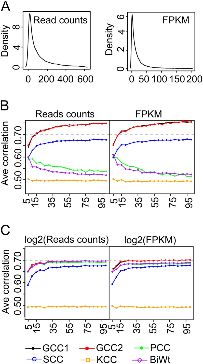
The compatibility of the five correlation methods on RNA-Seq data. A, The kernel density estimation of the read counts and the RPKM values were generated from the Arabidopsis RNA-Seq data (Gene Expression Omnibus accession nos. GSM838184 and GSM764078). By using the RNA-Seq data without (B) and with (C) log transformation, the average correlation coefficients of each method were calculated from 2,000 random gene pairs with an expected correlation coefficient of 0.70 across the five to 100 simulated samples. “Ave correlation” represents the average correlation coefficients.
Considering that most methods in microarray analyses use log transformation to scale the expression intensities to a proximal normal distribution, we next evaluated the five methods on the log2-transformed read counts and the FPKM. As for the read counts, the average correlations calculated by the GCC, PCC, and BiWt were all close to the expected 0.7 value (Fig. 5C). The performance of the SCC was not improved, since log transformation does not change the ranks of gene expression (Fig. 5C). When computing the correlations on log2-transformed FPKM values, the results from the GCC method are approximate to the expected value, while the average correlations from the PCC and BiWt were slightly below 0.7 (Fig. 5C). We speculate that calculating FPKM values from genes with very few reads may generate FPKM values below 1, and the log transformation resulted in negative values that influenced the accuracy of correlations. Collectively, our analyses showed that the GCC, PCC, and BiWt methods were equally effective on log2-transformed read counts, which can be recommended as the most optimal data form in RNA-Seq analysis.
Evaluation of the Five Methods Using 29 TF-Target Genes in Maize RNA-Seq data
Finally, we evaluated the five methods using a recently published RNA-Seq data set in maize (Zea mays) containing 13 samples that included eight male and female reproductive tissues, four tissues from developing seeds, and one leaf tissue (Davidson et al., 2011). Analyses were performed on three TFs (OUTER CELL LAYER1 [OC1], WRINKLED TRANSCRIPTION FACTOR [WRI], and MYB RELATED PROTEIN1 [MRP1]) functioning in these reproductive tissues and regulating 29 known target genes; this information was collected from a literature search (Supplemental Table S3). Correlations using these 29 pairs of TFs and targets were computed on the FPKM values using the five correlation methods (Supplemental Fig. S4), and the statistical significance (P value) was determined by the 2,000 permutation tests. The BiWt failed to calculate the correlations for six pairs of TF and target genes, since a number of samples had zero reads for these genes. The BiWt totally identified only seven TF-target interactions, which were much fewer than the numbers of TF-target interactions detected by the SCC (12), KCC (13), PCC (13), and GCC (17) methods with a P = 0.05 cutoff (Supplemental Fig. S4). All five methods failed to detect 12 pairs of TF-target interactions, including 10 pairs coexpressed in only one sample in either endosperm or anthers and two pairs exhibiting a lagged coexpression pattern (Supplemental Fig S5). These results indicated that all five methods require the regulatory relationships to concordantly present in at least two samples to be detectable.
Implementation of the Gini Correlation as an R Package for Gene Expression Clustering Analyses of Transcriptomic Data
Clustering analyses of gene expression patterns are an essential part of large-scale transcriptome analyses, which are usually performed with hierarchical clustering methods that measure the distance between two genes based on correlation coefficients (D’haeseleer, 2005). We implemented the Gini correlation method and four other correlation methods evaluated in this study in an R package, named rsgcc, to perform clustering analyses of both microarray data and RNA-Seq data based on either read counts or FPKM values and to visualize the clustered gene expression pattern using a heat map. This package is also capable of performing parallel computing to increase the speed of the calculation of correlation coefficients for thousands of genes via the implementation of the snowfall package in the R environment. Additionally, we also provided a user-friendly interface using the gWidgetsRGtk2 package in R, which allows users to perform analyses via a series of mouse actions without command line-based R programming (Fig. 6). The rsgcc package allows a user to easily select different correlation and clustering methods, to specify the number of central processing units for parallel computing, and to choose the color scales for heat map visualization (Fig. 6). In the current version of rsgcc, three types of distance measurements (raw correlation, 1-coef; absolute correlation, 1-|coef|; squared correlation, 1-|coef|2, where coef = correlation coefficient) and seven clustering methods (complete-linkage, average-linkage, median-linkage, centroid-linkage, McQuitty-linkage, single-linkage, and ward-linkage) are provided for users to select a variety of clustering methods.
Figure 6.

A screen shot of the GCC-based R package (rsgcc) for correlation and clustering analyses of gene expression data. The rsgcc was applied to cluster approximately 2,800 tissue-specifically expressed genes in maize RNA-Seq data. DAP, Days after pollination; Endo, endosperm; Post-em, postemergence; Pre-em, preemergence; ts-genes, tissue-specific genes.
Although the rsgcc is efficient in performing clustering analyses on all of the genes in a genome by taking advantage of parallel computing, preselecting a group of differentially expressed genes identified by Cufflinks or EdgeR or a group of tissue-specifically expressed genes to generate the clustered heat map is highly recommended. Therefore, we provided a function in rsgcc to select tissue-specific genes by calculating a tissue-specificity (ts) score for each gene. The detailed tissue-specificity algorithm is described in the online manual of rsgcc. To demonstrate the function of rsgcc, we first used the “find ts-genes” function to select a group of 2,279 tissue-specifically expressed genes out of the 39,456 genes from the RNA-Seq data profiled in 13 reproductive samples in maize (Davidson et al., 2011). Then, using the GCC-based similarity measure, a heat map of the 2,279 clustered, tissue-specific genes was generated by rsgcc in which the genes specifically expressed in the same tissue were successfully clustered in one group (Fig. 6). The clustered gene expression pattern can be saved in a standard output of the hierarchical clustering result: the “CDT” format, which can also be visualized and analyzed using the TreeView program (Saldanha, 2004). The rsgcc package and manual documents can be freely accessed from the Comprehensive R Archive Network at http://cran.r-project.org/web/packages/rsgcc.
CONCLUSION
In this study, we compared five correlation methods, the PCC, the SCC, the KCC, the BiWt correlation, and the GCC, in terms of effectiveness in inferring regulatory relationships from gene expression data. The evaluation analyses were performed based on known TF and target interactions collected from Arabidopsis and maize. Among these methods, the GCC was introduced in plants to our knowledge for the first time to analyze the transcriptomic data produced from microarray and RNA-Seq platforms. Compared with the other four methods, one of the unique features for the Gini correlation is that its algorithm reciprocally considers value and rank information of a TF and target pair, making the Gini correlation less dependent on the form of data distribution. This feature allows the Gini correlation to identify nonlinear relationships between TFs and targets, and transient interactions occurred in a small subset of samples, which might be missed by the methods that only globally consider value or rank information from all the samples. The robustness of the Gini correlation is also reflected in its higher tolerance of outlier data points and less dependence on sample size.
Application of the Gini correlation provides an alternative for biologists to analyze gene expression data. We implemented the Gini correlation as an R package to perform clustering analyses based on microarray data and RNA-Seq data. Additionally, this package can also be applied to construct gene coexpression networks and to perform network analyses on other types of interaction data. For instance, the rsgcc package is available to be called by the wgcna (weighted gene coexpression network analysis) package in the R environment (Langfelder and Horvath, 2008). This package can also be incorporated to the Cytoscape software as a plugin for broader utilization in network visualization and network analysis in biology (Smoot et al., 2011). Moreover, the Gini-based methodologies are a system of mathematical solutions, including the Gini correlation, Gini mean difference, Gini index, Gini covariance, and Gini regression, that can be used for a variety of purposes when analyzing data that are not distributed normally, and they are widely used in other disciplines, such as economics, physics, informatics, and sociology. Therefore, the Gini methodological systems have a promising prospect to model the complexity of biological systems.
MATERIALS AND METHODS
Microarray and RNA-Seq Data Sets
The microarray gene expression data were downloaded from the AtGenExpress database (http://www.weigelworld.org/resources/microarray/AtGenExpress/), which includes 79 samples that were collected during Arabidopsis (Arabidopsis thaliana) development. The microarray data were generated with the Affymetrix ATH1 array platform and have been normalized with the GC robust multiarray average method. More details about this microarray data set can be found in Schmid et al. (2005).
The maize (Zea mays) RNA-Seq data were obtained from Davidson et al. (2011), which contains 13 samples from eight reproductive tissues, four tissues from developing seeds, and one leaf tissue. The sequence reads of these tissue samples were first generated using the Illumina sequencing platform and then aligned to the maize genome (B73) by using the Bowtie and TopHat alignment tools with the limit of intron length ranging from 5 to 60,000 bp. The normalized gene expression levels in the FPKM format were finally calculated with the Cufflinks software. Detailed information about this RNA-Seq data set can be found in Davidson et al. (2011).
Computation of the GCC
The GCC is a well-defined measure to quantify the correlation between two variables following normal and/or nonnormal distributions (Schechtman and Yitzhaki, 1999; Yitzhaki, 2003). As the GCC method reciprocally utilizes the value information of one variable and the rank information of the other variable, it can produce two correlation coefficients. For a given gene pair (X, Y), one GCC is defined as
where n is the sample size (i.e. the number of observed gene expression values) and x(i, X) is the ith value of gene expression profile X sorted in an increasing order, here x(1, X) ≤ x(2, X) ≤ … ≤ x(i, X) ≤ … ≤ x(n, X). x(i, Y) is the corresponding value of X in the gene pair (X, Y) for the ith value of gene expression profile Y sorted in an increasing order.
The other GCC value can be given as
where y(i, X) and y(i, Y) are defined similarly to x(i, Y) and x(i, X), respectively, in Equation 1.
According to Equations 1 and 2, correlations of the GCC method can be interpreted as differences between two curves weighted by the information deriving from the rank order of gene expression data. The x(i, Y) and y(i, X) values are represented as red and blue curves in the last two columns, whereas x(i, X) and y(i,Y) are represented as black curves in these columns, in Figure 2.
Determining Statistical Significance
The statistical significance (P value) of the correlation was computed with the permutation test method (Qian et al., 2001; Wang et al., 2008). For one given gene pair and correlation method, the P value was calculated as follows. (1) Computing the correlation r on the real paired expression values. (2) Constructing a permuted gene pair by randomly shuffling gene expression data in different samples and recomputing the correlation on the permuted gene pair. (3) Repeating step 2 for a large number of times (n = 2,000), an empirical distribution (H0) of the correlations on the permuted gene pairs is then generated. (4) Calculating the statistical significance of the correlation r under the empirical distribution H0 with the formula P = 2 × m/N, where m denotes the times that the absolute value of the correlation on the shuffled data is greater than the correlation on the real data.
Supplemental Data
The following materials are available in the online version of this article.
Supplemental Figure S1. Scatterplots of GCC1 versus GCC2 for TF-target, TF-cofactor, and cofactor-target gene pairs.
Supplemental Figure S2. Venn diagrams of detected regulatory relationships with GCC, SCC, PCC, and BiWt at the significance level of P = 0.05.
Supplemental Figure S3. Number of gene pairs versus number of outliers.
Supplemental Figure S4. Correlations of 29 TF-target gene pairs computed by the five correlation methods.
Supplemental Figure S5. Gene expression profiles of 12 TF-target gene pairs missed by all tested correlation methods.
Supplemental Table S1. Statistics of the complied data set including known transcriptional regulation relationships in Arabidopsis collected from the AtTFDB database.
Supplemental Table S2. Influence of outliers on the performance of different correlation methods.
Supplemental Table S3. List of the 29 TF-target interactions from maize.
Supplementary Material
Glossary
- PCC
Pearson’s product-moment correlation coefficient
- SCC
Spearman’s rank correlation coefficient
- KCC
Kendall’s rank correlation coefficient
- TF
transcription factor
- GCC
Gini correlation coefficient
- BiWt
Tukey’s biweight
- ROC
receiver operating characteristic
- FPR
false positive rate
- TPR
true positive rate
- AUC
area under the ROC curve
- FPKM
fragments per kilobase per million reads
References
- Allen JD, Xie Y, Chen M, Girard L, Xiao G. (2012) Comparing statistical methods for constructing large scale gene networks. PLoS ONE 7: e29348. [DOI] [PMC free article] [PubMed] [Google Scholar]
- Arabidopsis Interactome Mapping Consortium (2011) Evidence for network evolution in an Arabidopsis interactome map. Science 333: 601–607 [DOI] [PMC free article] [PubMed] [Google Scholar]
- Berri S, Abbruscato P, Faivre-Rampant O, Brasileiro AC, Fumasoni I, Satoh K, Kikuchi S, Mizzi L, Morandini P, Pè ME, et al. (2009) Characterization of WRKY co-regulatory networks in rice and Arabidopsis. BMC Plant Biol 9: 120. [DOI] [PMC free article] [PubMed] [Google Scholar]
- Davidson RM, Hansey CN, Gowda M, Childs KL, Lin HN, Vaillancourt B, Sekhon RS, Leon ND, Kaeppler SM, Jiang N, et al. (2011) Utility of RNA sequencing for analysis of maize reproductive transcriptomes. Plant Genome 4: 191–203 [Google Scholar]
- D’haeseleer P. (2005) How does gene expression clustering work? Nat Biotechnol 23: 1499–1501 [DOI] [PubMed] [Google Scholar]
- Ficklin SP, Feltus FA. (2011) Gene coexpression network alignment and conservation of gene modules between two grass species: maize and rice. Plant Physiol 156: 1244–1256 [DOI] [PMC free article] [PubMed] [Google Scholar]
- Garber M, Grabherr MG, Guttman M, Trapnell C. (2011) Computational methods for transcriptome annotation and quantification using RNA-seq. Nat Methods 8: 469–477 [DOI] [PubMed] [Google Scholar]
- Hardin J, Mitani A, Hicks L, VanKoten B. (2007) A robust measure of correlation between two genes on a microarray. BMC Bioinformatics 8: 220. [DOI] [PMC free article] [PubMed] [Google Scholar]
- Hu M, Zhu Y, Taylor JM, Liu JS, Qin ZS. (2012) Using Poisson mixed-effects model to quantify transcript-level gene expression in RNA-Seq. Bioinformatics 28: 63–68 [DOI] [PMC free article] [PubMed] [Google Scholar]
- Jørstad TS, Langaas M, Bones AM. (2007) Understanding sample size: what determines the required number of microarrays for an experiment? Trends Plant Sci 12: 46–50 [DOI] [PubMed] [Google Scholar]
- Langfelder P, Horvath S. (2008) WGCNA: an R package for weighted correlation network analysis. BMC Bioinformatics 9: 559. [DOI] [PMC free article] [PubMed] [Google Scholar]
- Long TA, Brady SM, Benfey PN. (2008) Systems approaches to identifying gene regulatory networks in plants. Annu Rev Cell Dev Biol 24: 81–103 [DOI] [PMC free article] [PubMed] [Google Scholar]
- Ma C, Zhou Y, Huang SH. (2011) Inequalities and duality in gene coexpression networks of HIV-1 infection revealed by the combination of the double-connectivity approach and the Gini’s method. J Biomed Biotechnol 2011: 926407. [DOI] [PMC free article] [PubMed] [Google Scholar]
- Ma S, Gong Q, Bohnert HJ. (2007) An Arabidopsis gene network based on the graphical Gaussian model. Genome Res 17: 1614–1625 [DOI] [PMC free article] [PubMed] [Google Scholar]
- Marbach D, Prill RJ, Schaffter T, Mattiussi C, Floreano D, Stolovitzky G. (2010) Revealing strengths and weaknesses of methods for gene network inference. Proc Natl Acad Sci USA 107: 6286–6291 [DOI] [PMC free article] [PubMed] [Google Scholar]
- Moreno-Risueno MA, Busch W, Benfey PN. (2010) Omics meet networks: using systems approaches to infer regulatory networks in plants. Curr Opin Plant Biol 13: 126–131 [DOI] [PMC free article] [PubMed] [Google Scholar]
- Mortazavi A, Williams BA, McCue K, Schaeffer L, Wold B. (2008) Mapping and quantifying mammalian transcriptomes by RNA-Seq. Nat Methods 5: 621–628 [DOI] [PubMed] [Google Scholar]
- Nakashima K, Ito Y, Yamaguchi-Shinozaki K. (2009) Transcriptional regulatory networks in response to abiotic stresses in Arabidopsis and grasses. Plant Physiol 149: 88–95 [DOI] [PMC free article] [PubMed] [Google Scholar]
- Qian J, Dolled-Filhart M, Lin J, Yu H, Gerstein M. (2001) Beyond synexpression relationships: local clustering of time-shifted and inverted gene expression profiles identifies new, biologically relevant interactions. J Mol Biol 314: 1053–1066 [DOI] [PubMed] [Google Scholar]
- Reshef DN, Reshef YA, Finucane HK, Grossman SR, McVean G, Turnbaugh PJ, Lander ES, Mitzenmacher M, Sabeti PC. (2011) Detecting novel associations in large data sets. Science 334: 1518–1524 [DOI] [PMC free article] [PubMed] [Google Scholar]
- Rice JJ, Tu Y, Stolovitzky G. (2005) Reconstructing biological networks using conditional correlation analysis. Bioinformatics 21: 765–773 [DOI] [PubMed] [Google Scholar]
- Robinson MD, McCarthy DJ, Smyth GK. (2010) edgeR: a Bioconductor package for differential expression analysis of digital gene expression data. Bioinformatics 26: 139–140 [DOI] [PMC free article] [PubMed] [Google Scholar]
- Saldanha AJ. (2004) Java Treeview: extensible visualization of microarray data. Bioinformatics 20: 3246–3248 [DOI] [PubMed] [Google Scholar]
- Schechtman E, Yitzhaki S. (1999) On the proper bounds of the Gini correlation. Econ Lett 63: 133–138 [Google Scholar]
- Scheinine A, Mentzen WI, Fotia G, Pieroni E, Maggio F, Mancosu G, de la Fuente A. (2009) Inferring gene networks: dream or nightmare? Ann N Y Acad Sci 1158: 287–301 [DOI] [PubMed] [Google Scholar]
- Schmid M, Davison TS, Henz SR, Pape UJ, Demar M, Vingron M, Schölkopf B, Weigel D, Lohmann JU. (2005) A gene expression map of Arabidopsis thaliana development. Nat Genet 37: 501–506 [DOI] [PubMed] [Google Scholar]
- Smoot ME, Ono K, Ruscheinski J, Wang PL, Ideker T. (2011) Cytoscape 2.8: new features for data integration and network visualization. Bioinformatics 27: 431–432 [DOI] [PMC free article] [PubMed] [Google Scholar]
- Trapnell C, Williams BA, Pertea G, Mortazavi A, Kwan G, van Baren MJ, Salzberg SL, Wold BJ, Pachter L. (2010) Transcript assembly and quantification by RNA-Seq reveals unannotated transcripts and isoform switching during cell differentiation. Nat Biotechnol 28: 511–515 [DOI] [PMC free article] [PubMed] [Google Scholar]
- Usadel B, Obayashi T, Mutwil M, Giorgi FM, Bassel GW, Tanimoto M, Chow A, Steinhauser D, Persson S, Provart NJ. (2009) Co-expression tools for plant biology: opportunities for hypothesis generation and caveats. Plant Cell Environ 32: 1633–1651 [DOI] [PubMed] [Google Scholar]
- Vandepoele K, Quimbaya M, Casneuf T, De Veylder L, Van de Peer Y. (2009) Unraveling transcriptional control in Arabidopsis using cis-regulatory elements and coexpression networks. Plant Physiol 150: 535–546 [DOI] [PMC free article] [PubMed] [Google Scholar]
- Wang H, Wang Q, Li X, Shen B, Ding M, Shen Z. (2008) Towards patterns tree of gene coexpression in eukaryotic species. Bioinformatics 24: 1367–1373 [DOI] [PubMed] [Google Scholar]
- Wang Z, Gerstein M, Snyder M. (2009) RNA-Seq: a revolutionary tool for transcriptomics. Nat Rev Genet 10: 57–63 [DOI] [PMC free article] [PubMed] [Google Scholar]
- Wellmer F, Riechmann JL. (2010) Gene networks controlling the initiation of flower development. Trends Genet 26: 519–527 [DOI] [PubMed] [Google Scholar]
- Yilmaz A, Mejia-Guerra MK, Kurz K, Liang X, Welch L, Grotewold E. (2011) AGRIS: the Arabidopsis gene regulatory information server, an update. Nucleic Acids Res 39: D1118–D1122 [DOI] [PMC free article] [PubMed] [Google Scholar]
- Yitzhaki S. (2003) Gini’s mean difference: a superior measure of variability for non-normal distributions. METRON International Journal of Statistics LXI: 285–316 [Google Scholar]
- Yu H, Luscombe NM, Qian J, Gerstein M. (2003) Genomic analysis of gene expression relationships in transcriptional regulatory networks. Trends Genet 19: 422–427 [DOI] [PubMed] [Google Scholar]
Associated Data
This section collects any data citations, data availability statements, or supplementary materials included in this article.